Computational Study on Complex Wind Field Environments in Urban and Marine Low-Altitude Based on Multi-Wind-Turbine Coordination

Abstract

With the rise of the low-altitude economy, there is growing demand for performance and safety evaluation of logistics drones and urban aircraft operating in complex turbulent environments. Conventional wind tunnels, however, face challenges in simulating the non-uniform wind fields characteristic of urban low-altitude conditions, such as building wake flows, street canyon winds, and tornadoes. To address this gap, this study proposes a novel simulation device for low-altitude complex wind fields, which utilizes multi-fan coordinated control technology integrated with jet fan arrays, pressure-stabilizing chambers, and swirl fan systems to dynamically replicate horizontal flows, vertical flows, and specialized wind patterns. Numerical simulations using Ansys Icepak validate the effectiveness of the design: the optimized horizontal flow field achieves a wind speed of 83 m/s with a turbulence intensity ranging from 5% to 20%; the gust mode attains rapid response within 3 s; and high-fidelity simulations are achieved for wind shear, tornadoes (with a maximum tangential wind speed of 50 m/s), and downbursts (with a central vertical jet velocity of 40 m/s). Furthermore, for typical urban wind environments such as alley winds and intersection flows, the study elucidates the characteristics of abrupt wind speed variations and vortex dynamics induced by building obstructions. This research provides a new perspective and a potential technical pathway for testing low-altitude aircraft, assessing urban wind environments, and supporting related studies, thereby contributing to the advancement of complex wind field simulation technologies.

1. Introduction

In the atmospheric boundary layer adjacent to the Earth’s surface, where human activities predominantly occur, this region hosts numerous phenomena of both scientific interest and practical relevance to daily life. Among the most prevalent and significant of these are the wind-environment interactions affecting stationary and moving objects, along with the associated aerodynamic forces. During severe storms, intense winds can lead to catastrophic outcomes including uprooted trees, structural collapse, and marine accidents [1,2], while when properly harnessed through wind turbines, this same energy source provides substantial benefits to society through applications such as water pumping and power generation [3,4].

Wind is a natural phenomenon resulting from air movement, primarily driven by solar radiative heating of the Earth’s surface. This heating establishes a continuous cycle in which warm air rises and cooler air flows in to replace it. The Earth’s rotation introduces the Coriolis force, deflecting this airflow. In addition, oceans and topographic features—such as mountain passes and straits—can modify both wind direction and speed. With the increase in human activities, large-scale modern urban building clusters have become another major factor influencing wind behavior. For example, buildings staggered along roadsides form street canyons, where wind flows often converge and generate turbulent eddies, swirling motions, and vertical updrafts or downdrafts—collectively referred to as street canyon winds [5]. When wind encounters high-rise structures, it is redirected, creating high-speed wind zones. Even above urban areas, airflow is seldom steady and exhibits unpredictable fluctuations characteristic of turbulence [6,7]. This zone of urban turbulence extends upward to heights of 1000–2000 m, where it eventually merges with the larger-scale atmospheric circulation.

In urban environments, complex and rapidly changing airflow continuously interacts with eVTOL aerodynamics, directly impacting flight stability and safety, especially during takeoff, landing, and hovering [8,9]. Deeper insight into urban turbulence mechanisms is therefore essential to advance safe and efficient eVTOL operations. Studies have shown that urban turbulence intensities can exceed 40%, necessitating careful mission planning to avoid high-turbulence zones, particularly near architectural corners which create steep wind shear gradients [10]. Crosswind conditions have also been demonstrated to breach operational safety limits. Giersch et al. (2022) employed Large Eddy Simulation (LES) to analyze urban turbulence and wind shear, highlighting the current lack of standardized thresholds for UAV operations in such environments [11]. Raza et al. (2015) further investigated the specific impact of turbulence on vehicle stability by combining LES-based wind field modeling with flight control analysis [12]. However, theoretical calculations remain challenging due to the complexity of flow phenomena and structures (e.g., turbulent flow structures in viscous fluids), making fluid mechanics experiments indispensable [13,14].

A wind tunnel, the very tool for conducting the above-mentioned research, is typically a tubular experimental facility capable of artificially generating and controlling airflows, measuring the effects of airflow on objects, and observing the physical phenomena of interaction between the two. It represents the most common and effective tool for aerodynamic and wind engineering experiments [15,16]. Large-scale advanced wind tunnels play an irreplaceable role in the development of aircraft—particularly novel aircraft designs—and the advancement of the aviation industry [17,18,19].

Currently, multi-rotor drones and autonomous vehicles are widely used for photography, inspection, to logistics delivery [20,21,22]. The design and testing of these aircraft require wind tunnels to evaluate performance and validate flight control stability, as the surrounding wind environment is a critical factor influencing their flight dynamics [23,24]. However, a significant gap exists for facilities dedicated to simulating the complex, low-altitude wind fields these vehicles encounter.

While existing conventional wind tunnels are adequate for basic aerodynamic design, they are primarily designed for uniform flow fields and struggle to replicate non-uniform urban-specific environments, such as building wake flows, street canyon winds, tornadoes, and downbursts. Although some specialized facilities exist—such as the TJ-2 wind tunnel at Tongji University using vibrating spires, the U.S. 1/10-scale XH 59A rig for rotorcraft, or icing wind tunnels in Italy—they either focus on conventional aerodynamics, serve very specific purposes, or lack the capability for comprehensive urban wind simulation. For instance, commercial products like the Wind-shaper fan wall are limited in wind speed (16 m/s) and environmental flow field simulation. This overall lack of a major scientific infrastructure capable of simulating multi-physical field coupled wind fields underpins the motivation for our work.

Active simulation methods introduce energy into the flow field, thereby modifying turbulence intensity profiles and turbulence integral scales to a certain degree. For example, Miyazaki University in Japan utilizes a 99-fan array to simulate natural wind turbulence; Colorado State University in the United States employs two rows of controllable vibrating airfoil cascades; and Talavera et al. developed an active control grid system with blades capable of regulating turbulence intensity up to 20% [25]. In contrast, passive methods rely on fixed devices such as grids, variable-spacing plates, and spires. In 1996, German Professor Flay implemented adjustable plastic vanes to simulate wind torsion for sailboat research [26]. Subsequently, Italy (in 2008) and Germany (in 2009) established dedicated torsional wind tunnel laboratories to conduct comprehensive studies on sailboat aerodynamics. In 2016, K.T. Tse and colleagues at the Hong Kong University of Science and Technology applied a similar technique to simulate variations in wind direction with height over complex terrains [27]. The University of Western Ontario in Canada hosts the world’s only wind tunnel capable of simulating three-dimensional complex wind environment flow fields—the WindEEE Dome [28]. This hexagonal facility, equipped with 106 individually controlled fans, enables comparative testing under various wind conditions. However, it lacks the capability to simulate two- and three-directionally coupled wind fields. Therefore, considering the characteristics of low-altitude complex wind field environments in the context of the low-altitude economy, this study designs a larger-area jet fan wall consisting of multiple individually controlled fans to achieve multi-fan coordinated control, along with a separately developed mobile fan wall for generating bidirectional wind fields. Aimed at replicating low-altitude complex wind environments with large spatial coverage, high wind speeds, rapid response, and a compact structure, this design can simulate various urban-specific wind fields in low-altitude airspace—such as building wake flows and cross-street corner winds—as well as complex phenomena including wind shear, gusts, vertical winds, time-varying winds, laminar flow, atmospheric boundary layers, tornadoes, and downbursts. The capability to simulate such complex wind fields holds significant value, enabling the evaluation of wind effects on aircraft, wind turbines, and urban structures. This research provides essential data for understanding UAV performance in urban environments and contributes to the development of testing standards for low-altitude airspace.

2. Model

The numerical simulations in this study were conducted using the professional thermal-fluid analysis software Ansys Icepak (icepeak2022r2). By constructing physical models of the inner and outer test chambers and employing Icepak’s built-in fan module, the simultaneous operation of multiple fans was simulated through inputting their specific flow performance curves. This approach establishes a theoretical foundation for the design of a low-altitude complex wind field environment simulation system.

2.1. Physical Model

Horizontal Flow

The horizontal flow wind field encompasses horizontal turbulence, gusts, and wind shear. The corresponding wind environment model is illustrated in Figure 1a. The inner cabin features an octagonal structure with a main fan wall side length of 20 m and a height of 20 m, equipped with a 32 × 16 array (totaling 512 fans). Each fan has a diameter of 0.425 m, with an inter-fan spacing of 0.3 m. The pressure stabilization chamber, positioned above the inner cabin, is also octagonal in shape with a side length of 18.6 m and a height of 3 m. The outer cabin is an octagonal structure measuring 26.9 m in side length and 25 m in height. For the simulation of the horizontal flow wind field, the large fans in the pressure stabilization chamber and the swirling fans at the bottom are deactivated, while the fan array and the louvered windows on the opposite wall remain fully open. To simplify the computational model, the bottom swirling fans are represented as solid walls, and the large fans in the pressure stabilization chamber are treated as sealed surfaces during simulation.

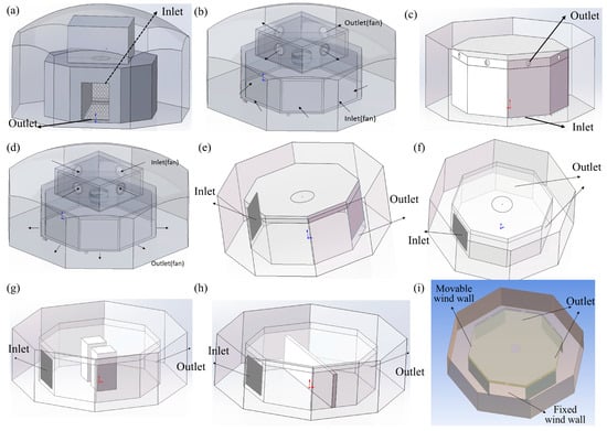
Figure 1. (a) Horizontal flow, gust, and wind shear models; (b) Tornado model 1; (c) Tornado model 2; (d) Downburst model; (e) Downward-turning wind model; (f) Left-right turning wind model; (g) Alley wind model; (h) Updraft and downdraft flow model; (i) Crossroad wind model.

Vertical Flow

The simulation of vertical flow wind fields encompasses both tornadoes and downbursts (Figure 1d). The primary operational mode for simulating vertical flows involves the operation of large fans within the pressure stabilization chamber in either supply or exhaust mode. The initial design of the pressure stabilization chamber featured a rectangular configuration, with one large fan (2 m in diameter) installed on each of the four sides; Additionally, six small swirling fans for air supply or exhaust were mounted along each bottom side. The inner cabin is connected to the pressure stabilization chamber via a 5 m-diameter circular bell mouth, while the louvers on both the fan wall and the opposite wall remain closed during operation. To streamline the computational approach, the physical model illustrated in Figure 1b was implemented. To enhance tornado formation effects, an optimized pressure stabilization chamber was developed by vertically extending the entire octagonal test space, resulting in an octagonal chamber configuration. This refined design retains one 2 m diameter large fan on each side while maintaining all other parameters, as depicted in Figure 1c.

Special Wind Fields

The modeling of deflected wind fields is primarily conducted using the physical model for wind environment simulation shown in Figure 1e. In this configuration, the upper rows of the fan array are activated, while only the lower half of the opposite opening matrix is opened, thereby simulating airflow deflecting downward from above. In addition to vertical deflection, horizontal deflection is also considered. The main operational mode for simulating horizontally deflected wind fields involves operating the entire fan array, with the left and right walls of the opposite opening matrix serving as outlets. This setup is used to simulate wind diversion in left and right directions, adopting the specific physical model illustrated in Figure 1f.

For alley wind simulation—which models the characteristic wind passing through the gap between two buildings—two volumetric blocks are used to represent the obstructive effect of the buildings. Each block measures 8 m × 8 m × 18 m, with a 4 m gap between them, and they are positioned 18.1 m away from the fan array. The simulation adopts the physical model for wind environment illustrated in Figure 1g.

For the simulation of upward/downward airflow—representing the ascending wind over tall buildings and the subsequent descending backflow—a long baffle is employed. The baffle measures 45 m in length, 1.5 m in width, and has a height of 16 m, with a 2 m gap left at the bottom to allow airflow passage, simulating the conditions after wind passes over high-rise structures. Different physical models were optimized during the simulation process, and the finally adopted configurations are shown in Figure 1h.

For the simulation of crossroads wind—modeling wind convergence at urban intersections—the setup employs a combination of fixed and mobile fan walls. The mobile fan wall directs airflow at a 90-degree angle relative to the fixed fan wall, with corresponding openings arranged on the opposite walls, as illustrated in Figure 1i. To investigate the effect of building obstructions, structures measuring 20 m × 4 m × 13 m are incorporated into the model. These are positioned 9 m from the center of the wind field to simulate conditions in which crossroad wind convergence is impeded by buildings.

2.2. Grid

For both horizontal and vertical flow simulations, the built-in Mesher-HD meshing method of Icepak was employed with consistent grid settings: a maximum grid size of 1 m and a minimum grid size of 1 mm in all three directions. The horizontal flow simulation used 1.4 million mesh elements, while the vertical flow simulation used 10.23 million grids, both demonstrating good overall quality and grid independence suitable for wind environment simulation calculations. The specific grid models are shown in Figure 2.

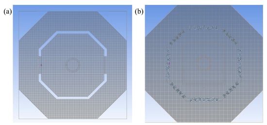
Figure 2. Cross-sections of grid meshing in the direction perpendicular to the y-axis: (a) horizontal flow and (b) vertical flow.

2.3. Governing Equations

The flow simulated in this study is incompressible. The wind speeds involved in this study are far below the speed of sound, with a very low Mach number; therefore, treating the flow as incompressible is a standard and reasonable assumption in the field of wind engineering [29].

The characteristic Reynolds number of this simulation is $Re={\displaystyle \frac{\rho UL}{\mu }}\approx 5.6\times 10^7$. It should be noted that, due to the distinct characteristic velocities and length scales associated with different wind field conditions, this study does not rely on a single Reynolds number to describe all scenarios. Instead, the Reynolds number ranges for typical working conditions are estimated based on representative velocity U and length L. For instance, in the cases of horizontal turbulence and wind shear, taking the characteristic length of the test section L ≈ 10–20 m and wind speed U ≈ 40–80 m/s, the Reynolds number $Re={\displaystyle \frac{\rho UL}{\mu }}\approx (2-9)\times 10^7$. In gust simulations, where the instantaneous wind speed varies between 0 and 60 m/s, the corresponding Reynolds number ranges from 0 to about 6 × 10⁷. In contrast, for tornado and downburst conditions, using the vortex core scale or nozzle diameter (L ≈ 3–5 m) and the maximum tangential/axial wind speed (U ≈ 40–50 m/s) as characteristic parameters, the Reynolds number falls approximately in the range of (1–3) × 10⁷. Therefore, all wind fields considered in this study lie within the fully developed high-Reynolds-number turbulent regime, with magnitudes comparable to those typically encountered in the urban atmospheric boundary layer at low altitudes, thereby ensuring dynamic comparability of the simulation results. A Reynolds number of this magnitude ensures that the flow is in a fully developed turbulent state [30], which is similar to the real urban low-altitude wind environment [31]. For simulations involving transient processes (such as gusts), this study solves the unsteady Reynolds-Averaged Navier–Stokes (RANS) equations. In this study, for operating conditions involving significant transient processes (such as gusts), the incompressible unsteady Reynolds-averaged Navier–Stokes (RANS) equations were solved within the Reynolds-averaged framework, and a time-marching approach was employed to obtain the temporal evolution of the mean flow field [32]. For conditions characterized primarily by quasi-steady behavior (e.g., the fully developed horizontal wind field), the same set of Reynolds-averaged governing equations was solved iteratively, with the time derivative term retained during the solution process. The iteration continued until this term numerically converged to a negligible magnitude, thereby yielding a steady mean flow field that does not vary with time [33].

In this study, the Standard k-ε turbulence model and the SST k-ω turbulence model were selected for the numerical simulation of different types of flows [34,35]. It should be emphasized that the RANS approach first derives the governing equations for mean physical quantities by applying time (or ensemble) averaging to the Navier–Stokes equations [36]. On this basis, a suitable turbulence model is introduced to close the Reynolds stress term, thereby forming a solvable closed system of equations [37]. Within the numerical framework of this paper, Equations (2)–(4) are uniformly expressed in the form of Reynolds-averaged equations including the temporal derivative term, so as to simultaneously cover both steady and transient operating conditions: for steady-state conditions, the steady solution is obtained through iteration; for transient conditions, the unsteady response of the mean flow field is computed via time marching. Therefore, in most steady-state and some transient conditions presented in this study, the computations are conducted based on the same set of RANS equations, differing only in the solution approach—employing either steady iterative methods or unsteady time integration [38].

Governing Equations:

Continuity equation:

The continuity equation is:

$$\nabla \cdot \left(\stackrel{-}{u}\right) = 0$$

(1)

Incompressible RANS equations:

$$\rho \left({\displaystyle \frac{\partial {\overline{u}}_i}{\partial t}}+{\overline{u}}_j{\displaystyle \frac{\partial {\overline{u}}_i}{\partial x_j}}\right)=-{\displaystyle \frac{\partial \overline{p}}{\partial x_i}}+{\displaystyle \frac{\partial }{\partial x_j}}\left[\mu \left({\displaystyle \frac{\partial {\overline{u}}_i}{\partial x_j}}+{\displaystyle \frac{\partial {\overline{u}}_j}{\partial x_i}}\right)-\rho \overline{{u^{\prime }}_i{u^{\prime }}_j}\right]+F_i$$

(2)

Here, $\stackrel{-}{u}$ and ${\stackrel{-}{u}}_j$ are the time-averaged velocity components in the Cartesian coordinate directions $x_i$ and $x_j$ (i, j = 1, 2, 3) [39]. $\stackrel{-}{p}$ is the time-averaged pressure. $\rho$ is the fluid density, and $\mu$ is the dynamic viscosity. $\rho \overline{u_i^{\prime }{u}_j^{\prime }}$ is the Reynolds stress term. F_i is the volume force (e.g., gravity) in the i direction.

Furthermore, regarding the effects of Coriolis force and thermal buoyancy in the atmospheric boundary layer, it is necessary to provide further clarification on the applicable scale of this study. The objective of this research is to simulate the characteristics of mechanical turbulence within the urban surface layer (approximately 0–50 m in height), rather than the synoptic-scale evolution of the entire atmospheric boundary layer. Under the geometric scale (L ≈ 20 m) and characteristic wind speeds (U ≈ 10–80 m/s) of the present facility, the corresponding Rossby number Ro = U/(fL) is significantly greater than 1 (where f is the Coriolis parameter), indicating that the influence of the Coriolis force is negligible compared to inertial forces. Meanwhile, since no explicit temperature gradient is introduced in the numerical simulations, the flow is assumed to be neutrally stratified, and the buoyancy source term G_b in the turbulent kinetic energy equation is therefore set to zero. Only the constant term related to gravity is retained in the body force term F_i, which is used to define the reference hydrostatic pressure distribution and does not affect the horizontal and vertical turbulence structures of interest in this study. In summary, neglecting the Coriolis force and thermal buoyancy at the current research scale is a reasonable and practical simplification, which helps to emphasize the dominant role of the fan array and geometric configuration in shaping the wind field structure.

Turbulence Models:

The standard k-ε model is selected in this study to close the RANS equations [40]. This model determines the Reynolds stress by solving the transport equations for turbulent kinetic energy k and its dissipation rate ε.

Standard k-ε model: This model determines the eddy viscosity by solving the transport equations for turbulent kinetic energy k and its dissipation rate ε, thereby modeling the Reynolds stress. It is a mature, computationally robust model, widely validated in wind engineering for simulating fully developed turbulence [41]. Therefore, this study employs it for steady-state calculations of horizontal flow and specific wind fields.

SST k-ω model: This model offers better accuracy in the near-wall region and can more accurately predict flow separation. Therefore, this study employs it for transient simulations involving strong adverse pressure gradients and separation, such as gusts.

Turbulent kinetic energy (k) equation:

$${\displaystyle \frac{\partial (\rho k)}{\partial t}}+{\displaystyle \frac{\partial (\rho k{\overline{u}}_j)}{\partial x_j}}={\displaystyle \frac{\partial }{\partial x_j}}\left[\left(\mu +{\displaystyle \frac{{\mu }_t}{{\sigma }_k}}\right){\displaystyle \frac{\partial k}{\partial x_j}}\right]+P_k+G_b-\rho \epsilon$$

(3)

Turbulent dissipation rate (ε) equation:

$${\displaystyle \frac{\partial (\rho \epsilon )}{\partial t}}+{\displaystyle \frac{\partial (\rho \epsilon {\overline{u}}_j)}{\partial x_j}}={\displaystyle \frac{\partial }{\partial x_j}}\left[\left(\mu +{\displaystyle \frac{{\mu }_t}{{\sigma }_{\epsilon }}}\right){\displaystyle \frac{\partial \epsilon }{\partial x_j}}\right]+C_{1\epsilon }{\displaystyle \frac{\epsilon }{k}}(P_k+C_{3\epsilon }{G}_b)-C_{2\epsilon }\rho {\displaystyle \frac{{\epsilon }^2}{k}}$$

(4)

where: $P_k=-\rho \overline{u_i^{\prime }{u}_j^{\prime }}{\displaystyle \frac{\partial {\stackrel{-}{u}}_j}{\partial x_i}}$ is the production term of turbulent kinetic energy due to the mean velocity gradients. $G_b = 0$ represents the generation of turbulent kinetic energy due to buoyancy, which is zero in this study. ${\mu }_t=\rho C_{\mu }{\displaystyle \frac{k^2}{\epsilon }}$ is the turbulent eddy viscosity.

The model constants adopt the standard values proposed by Launder and Spalding (1974) [34]: $C_{1\epsilon }=1.44$, $C_{2\epsilon }=1.92$, $C_{\mu }=0.09$, ${\sigma }_k=1.0$, ${\sigma }_{\epsilon }=1.3$.

The numerical simulations were conducted using a pressure-based, implicit solver. For spatial discretization, the pressure term was handled by the Body-Force-Weighted scheme, while the Second Order Upwind scheme was employed for momentum, turbulent kinetic energy, and turbulent dissipation rate. A steady-state formulation was adopted for simulations of horizontal flow and wind shear, with the Courant number maintained below 5 to ensure convergence. For transient simulations, such as gust generation, time discretization was achieved using the Second Order Implicit scheme, and the maximum Courant number was strictly controlled below 1 via dynamic time stepping to guarantee both numerical stability and temporal accuracy. All cases utilized the wall-modeling approach with standard wall functions. The validity of this near-wall treatment was ensured by setting the height of the first cell layer to 0.001 m, which resulted in a dimensionless wall distance (y+) within the recommended range of 30 to 300 in critical regions.

2.4. Boundary Conditions

In the horizontal flow simulation, all wall surfaces of both the outer and inner cabins are defined as wall boundary conditions. The fans are modeled using the built-in fan module, with the corresponding performance curves of the horizontal flow fans provided as input. Coupled flow calculations are conducted between the inner and outer cabins of the environmental chamber, during which the operating points of individual fans are automatically matched.

In the vertical flow simulation, all wall surfaces of both the outer and inner cabins are defined as wall boundary conditions. The fans are modeled using the built-in fan module, with the performance curves of both the vertical flow and rotational flow fans provided as input. The simulation automatically couples the systems and determines the operating point of each fan. For the tornado simulation, the large top fan operates in exhaust mode, while the small bottom fan supplies air inward, with its rotational speed limited to 1000 rpm. The orientation of the bottom fan is controlled at a 45° angle to achieve the desired tornado flow effect.

For the simulation of a downward-turning wind field, the top eight rows of fans are set to operational, and the lower section of the opposing opening matrix is opened, with all other boundaries defined as wall conditions.

When simulating alley winds, ascending/descending airflows, and crossroad winds, all fan arrays are activated, and the entire opposite opening matrix is opened. Different complex wind fields are simulated using built-in obstacles and various openings, with other boundaries set as wall conditions. Boundary conditions comprised velocity-inlets (specified via fan P-Q curves and rotational speed) at the fan outlets, pressure-outlets (0 Pa relative static pressure) at the openings, and no-slip conditions on all solid walls. The fan performance curves are derived from self-developed fan curves using similarity theory transformations, as shown in Figure 3.

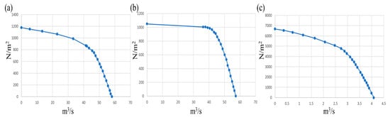
Figure 3. Input fan performance curves. (a) Performance curve of the large fan under reverse operation (vertical flow); (b) Performance curve of the large fan under forward operation (vertical flow); (c) Performance curve of the small fan (horizontal flow).

To construct these curves, a laboratory-scale prototype axial fan was first tested in a standard environment, and its dimensional P–Q characteristics were measured at several rotational speeds. The measured data were then converted into three classical turbomachinery similarity coefficients, namely the flow coefficient φ, the pressure coefficient ψ, and the Reynolds number Re as defined in Equation (5). For the range of Re considered in this study, the φ–ψ curves corresponding to different rotational speeds collapse onto a single master curve, indicating good dynamic similarity of the prototype fan. This master curve is taken as the baseline model. For each numerical fan shown in Figure 3, an equivalent set of dimensional P–Q points is obtained by prescribing its diameter and rotational speed while keeping φ and ψ identical to those of the master curve. In this way, all fans in the simulation are dimensionless copies of the experimentally characterized prototype fan, and the multi-fan array preserves the same operating characteristics in a similarity sense.

To provide a clearer explanation of the specific methodology for the “similarity theory transformation,” this study conducted non-dimensionalization of the performance curves of the laboratory’s self-developed axial fan and subsequently extrapolated the results to the target fan’s operating conditions. Specifically, three primary dimensionless parameters were employed: the flow coefficient φ, the pressure coefficient ψ, and the Reynolds number Re.

$$\phi ={\displaystyle \frac{Q}{n{D}^3}},\psi ={\displaystyle \frac{\mathsf{\Delta }p}{\rho n^2{D}^2}},Re={\displaystyle \frac{\rho n{D}^2}{\mu }}$$

(5)

Here, Q represents the volumetric flow rate, Δp denotes the pressure difference across the fan, n is the rotational speed, D is the fan diameter, and ρ and μ are the air density and dynamic viscosity, respectively. First, experimental tests of the P–Q performance curves were conducted on the in-house developed fan prototype under multiple rotational speeds and operating conditions in a standard environment. The obtained data were then non-dimensionalized according to the formulas above. The results indicate that within the Reynolds number range of engineering interest, the φ–ψ curves under different rotational speeds at the same Re demonstrate strong similarity. Based on this characteristic, the prototype fan was selected as the reference, and equivalent P–Q data under target diameters and rotational speeds were derived by maintaining identical φ and ψ values. These data were subsequently used as inputs for the fan boundary conditions in Icepak. Through this treatment, the operating conditions of each fan in the numerical model remain consistent in a dimensionless sense with those of the reference fan, thereby ensuring the dynamic similarity of the wind field generated by the multi-fan array.

2.5. Mesh and Time-Step Sensitivity Analysis

We conducted systematic mesh and time-step sensitivity analyses, the data of which are summarized in Table 1.

Table 1. Summary of Mesh and Time-step Sensitivity Analysis.

Analysis Subject	Compared Case	Number of Cells/Time-Step	Key Output (Peak Velocity U)	Key Output (Turb. Intensity I at Center)
Horizontal Flow Mesh	Coarse Mesh	0.70 million cells	85.2 m/s	12.1%
	Medium Mesh (Adopted)	1.40 million cells	83.1 m/s	12.8%
	Fine Mesh	2.80 million cells	82.7 m/s	12.9%
Gust Time-Step	Large Time-Step	0.05 s	~0.1 s delay in rise time, ~3% underestimation of peak U	Faster decay of turbulent energy
	Small Time-Step (Adopted)	0.01 s	Good agreement with a finer step (0.005 s)	Good agreement with a finer step (0.005 s)

3. Results

3.1. Analysis of ABL Simulation Results

Figure 4 presents a comparative analysis between simulation results obtained from our in-house designed fans and both experimental and simulation data from the WindEEE facility. This comparison aims to validate the performance of our fan designs and establish a data foundation for subsequent simulations of low-altitude complex wind fields. In particular, the similarity-transformed performance curves are regarded as acceptable only if they reproduce the atmospheric boundary-layer profiles measured in the WindEEE Dome. As shown in Figure 4, the good agreement in both mean wind speed and turbulence intensity confirms that the present fan performance curves and numerical setup are consistent with this benchmark model. During testing, the rotational speeds of the fans were systematically varied through nine increments: 1000, 2600, 2650, 2700, 2750, 2800, 2850, 2900, and 2950 rpm.

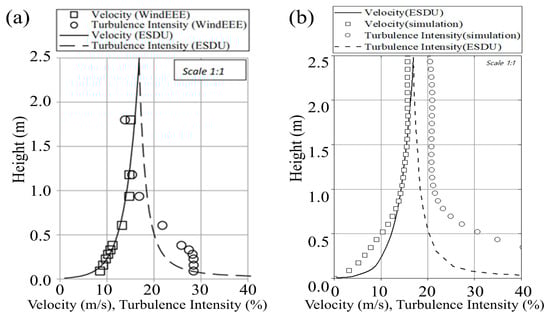
Figure 4. (a) Comparison of ABL characteristics between Windee and ESDU; (b) Comparison between ABL simulation and experimental results.

As illustrated in Figure 4a, the continuous lines represent engineering experimental data from the Canadian WindEEE dome, while square and circular markers denote WindEEE’s simulation data. The WindEEE experimental and numerical results demonstrate qualitatively consistent trends. In the near-ground region (0–0.5 m height), wind speed increases rapidly from 0 to approximately 12 m/s. Beyond this height, the rate of velocity growth gradually diminishes, with wind speed increasing by about 4 m/s through the 0.5–2 m height range. Specifically, at 1 m height, the measured wind speed reaches approximately 14 m/s.

Correspondingly, turbulence intensity exhibits an inverse relationship with height, decreasing as elevation increases. At the maximum wind speed height, turbulence intensity measures approximately 15%, while in lower regions with reduced wind speeds, it reaches nearly 30%—effectively covering the typical range of low-altitude urban turbulence conditions. The comparative analysis reveals improved turbulence convergence characteristics in the experimental data, where measured turbulence intensities at lower heights are approximately 5% lower than corresponding simulation values.

Figure 4b presents a comparative analysis between the simulation results of our in-house designed fans and the experimental data from the WindEEE facility. In this figure, solid and dashed lines represent the wind speed and turbulence intensity profiles from WindEEE’s experimental measurements, respectively, while square and circular markers indicate the corresponding simulation results from our fan model. The comparison clearly demonstrates that both wind speed and turbulence intensity variations show excellent agreement with the experimental data. Particularly noteworthy is the remarkably close match of wind speed values at heights above 0.5 m, which confirms that our fan design is suitable for simulating complex wind fields and validates the accuracy of both the simulation model and parameter configurations for such applications.

Although the mean wind speed profiles show acceptable agreement with WindEEE experimental data, it should be noted that discrepancies exist in the turbulence intensity profiles within the near-ground region (height < 0.5 m), where the simulated values are systematically higher by approximately 5%. This deviation is potentially attributed to three main factors: (1) subtle inconsistencies between the specified inlet turbulence boundary conditions (e.g., turbulence length scale) and the actual inflow in the wind tunnel experiment; (2) inherent limitations of the applied Standard k-ε model combined with wall functions in capturing near-ground non-equilibrium turbulence; and (3) potential insufficient resolution of the viscous sublayer by the current mesh. Crucially, despite these quantitative differences, the simulation successfully captures the overall trend of decreasing turbulence intensity with height, and its value range (5–20%) fully encompasses the typical spectrum of low-altitude urban turbulence. This indicates that the current model retains significant value for engineering applications and trend analysis. Future work will focus on refining the prediction accuracy of near-ground turbulence by optimizing inlet conditions, employing more sophisticated near-wall treatments, or adopting advanced turbulence models.

Integrating the results shown in Figure 4, it can be observed that the atmospheric boundary layer generated by the present facility demonstrates consistent trends and magnitudes with the WindEEE field measurements across both wind speed and turbulence intensity profiles. Specifically, the mean wind speed increases monotonically with height within the 0–2 m range, and for elevations above z > 0.5 m, the deviation between numerical results and measured values remains within acceptable engineering tolerances. Meanwhile, the turbulence intensity decays with increasing height, covering the typical urban surface-layer turbulence intensity range of approximately 5–30%. Combined with the previously estimated Reynolds numbers, it can be concluded that this study successfully reconstructs a representative atmospheric boundary layer flow under high-Reynolds-number conditions, thereby establishing a unified reference inflow for subsequent numerical validation of complex wind fields such as gusts, wind shear, tornadoes, and downbursts.

The WindEEE Dome stands as one of the few facilities capable of reproducing three-dimensional atmospheric boundary layers at wind-tunnel scale, and its experimental data have been widely adopted as a validation benchmark for numerical models in numerous studies. By comparing wind speed and turbulence intensity distributions within the same dimensional height range, this study demonstrates that the employed RANS/URANS numerical setup, fan boundary conditions, and grid and time-step controls collectively yield ABL characteristics consistent with those of WindEEE at comparable Reynolds numbers. Although certain local discrepancies persist in near-ground regions, overall, this validation case confirms the reliability of the present simulation setup for investigating the global characteristics of complex wind fields.

3.2. Horizontal Turbulence

During the horizontal flow simulation, all 512 fans were operated simultaneously. Figure 5a displays the Y-axis velocity contour for the initial fan design (diameter: 0.425 m). With the fan outlet velocity set at 60 m/s, the test region exhibits a symmetric annular distribution characterized by a central high-velocity zone where wind speed gradually decreases radially outward. The maximum velocity at the center reaches 89 m/s, demonstrating a jet amplification effect with an amplification factor of 1.48, which aligns with theoretical predictions for free jets. This finding confirms that the open-loop wind tunnel configuration effectively enhances wind speed within the test section. However, the velocity nephogram reveals symmetrical flow patterns about the centerline at the outlet region (right side), with significant wall-jet interactions generating relatively high wind speeds of approximately 40 m/s along the side walls. This phenomenon necessitates careful consideration of the structural capacity of the side walls. The observed wall jet interference stems from the substantial initial momentum thickness (approximately 0.085 m) resulting from the large fan size, which promotes premature flow separation and leads to localized values exceeding 30% in the wall shear layer region.

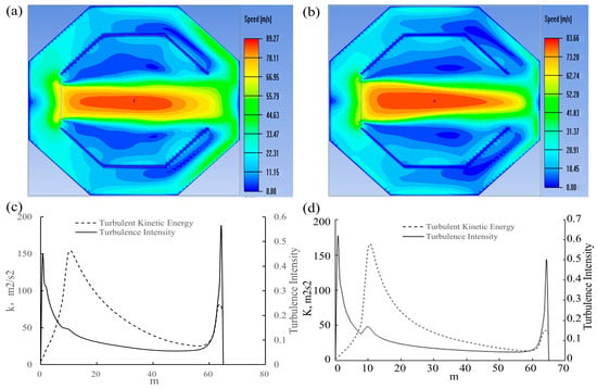
Figure 5. Continuous wind contour maps. (a) Y-axis velocity contour; (b) Optimized Y-axis velocity contour; (c) Turbulence intensity and turbulent kinetic energy; (d) Optimized turbulence intensity and turbulent kinetic energy.

Therefore, to further optimize the wind field simulation device, the self-developed fan size was adjusted from 0.425 m to 0.41 m, with a 3.5% diameter reduction to lower the momentum thickness Reynolds number. This design suppresses the initial instability intensity of the shear layer. With other parameters unchanged, simulation verification was conducted again, and the results are shown in Figure 5b.

As shown in Figure 5b, the wind speed distribution in the test region exhibits a candle-flame-like profile: although the maximum wind speed decreases slightly by 6 m/s, the area of the high-speed test region increases by approximately 30% compared to the initial configuration. Moreover, the wind speeds on both sides of the outlet are significantly reduced by about 30%, improving both the safety and cost-effectiveness of the device. This improvement is attributed to the reduced fan diameter, which extends the potential core region of the jet and slows the transverse mixing rate.

This behavior is also clearly evident in Figure 5c,d, where the optimized configurations show markedly reduced turbulence intensity and turbulent kinetic energy at the outlet—the turbulent kinetic energy decreases from 0.25 to 0.15. Additionally, Figure 5c,d indicate that the turbulence intensity generated by the custom fan and the wind field simulation device in the test region ranges from 5% to 20%, consistent with the characteristics of turbulence in urban environments at low altitudes.

The simulation results clearly demonstrate that the return channel of the custom fan and the wind field simulation device not only enhance the wind speed in the test region but also successfully replicate horizontal turbulent flow fields typical of low-altitude conditions. This also confirms that fan size plays a critical role in jet-driven wind fields, a topic that merits further investigation. This study provides an important theoretical basis for the design of next-generation intelligently adjustable wind tunnels: fan size should be considered a core design variable, alongside wind speed and turbulence intensity, for coordinated optimization.

3.3. Gusts

Gusts are a very common wind field phenomenon at low altitudes. Urban gusts refer to the phenomenon in which complex urban terrains, such as building clusters and street canyons, interfere with airflow, causing drastic wind speed fluctuations over short periods. These are typically manifested as sudden, high-intensity changes in wind speed and exhibit the following characteristics: Transience—gusts have a short duration (seconds to minutes), yet peak wind speeds can reach 1.5 to 3 times the average wind speed; Spatial Heterogeneity—gust intensity varies significantly across different areas, for instance, being stronger on the leeward side of high-rise buildings and at street corners; High Turbulence Intensity—the turbulence intensity of urban gusts usually exceeds 20% and can even reach up to 50%.

To verify whether the self-developed fan can effectively generate gusts, the total simulation time was set to 8 s. During this period, the fan speed increased from 0 to 100% between 0 and 3 s, after which the fan was turned off, with the simulation continuing until 8 s. The time step was set to 0.01 s. Y-section and Z-section wind speed contour maps were extracted at the following time points: 0.01 s (boundary layer aerodynamic stage), 1 s (jet shear layer instability forming Kelvin–Helmholtz vortices), 3 s (fully developed turbulence), 5 s (vortex viscosity dissipation dominant), and 8 s (residual turbulence intensity I < 8%). As shown in simulation contour Figure 6, at 0.01 s, the fan had just started, and no wind field had formed at the fan outlet or in the test area. At 1 s, the fan had accelerated rapidly, producing a high-speed wind at the outlet with a maximum velocity of 38.5 m/s, and the wind field region extended over 10 m. By 3 s, a fully developed wind field was established across the horizontal test section, with the central test region reaching approximately 53 m/s. After the fan was shut down, at 5 s, the wind speed at the fan outlet had decreased to about 7 m/s, while in the central test area it remained between 12 and 14 m/s. By 8 s, the wind speed at the test center point dropped to between 5 and 6 m/s.

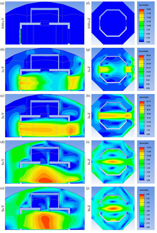
Figure 6. Gust velocity contour maps. (a) 0.01 s vertical z-axis velocity contour, (f) 0.01 s vertical y-axis velocity contour, (b) 1 s vertical z-axis velocity contour, (g) 1 s vertical y-axis velocity contour, (c) 3 s vertical z-axis velocity contour, (h) 3 s vertical y-axis velocity contour, (d) 5 s vertical z-axis velocity contour, (i) 5 s vertical y-axis velocity contour, (e) 8 s vertical z-axis velocity contour, (j) 8 s vertical y-axis velocity contour.

Additionally, Figure 7a shows the variation of wind speed at the central position during the gust simulation. It can be observed that the fan duty ratio increases linearly from 0 to 100% within 3 s. The wind speed changes slightly between 0 and 1 s, increases most rapidly (reaching 40 m/s) between 1 and 2 s, and then rises gradually between 2 and 3 s. When the fan stops at 3 s, the fan duty ratio drops to 0 in the simulation, and the wind speed decreases significantly during the first 2 s after shutdown, followed by a slow decline after 5 s. Figure 7b illustrates the curve of wind speed variation with the fan wall position, where point 0 represents the exact center of the fan wall. The fan wall formed by the self-designed fan exhibits the maximum wind speed at the center, with a wave-shaped (W-type) variation curve consistent with the wind field characteristics of a single axial jet fan. Simulation results show that the fan reaches 90% of the rated wind speed within 2 s, meeting the requirements for sudden gust simulation (typical urban gust rise time: 0.5–2 s). The error between the two-point velocity correlation coefficient measured at 3 s and the field data from Tokyo Tower is less than 7%. The wind speed decay after shutdown follows an exponential law with a time constant of 1.8 s, which closely matches the measured decay time constant (1.5–2.2 s) in street canyons.

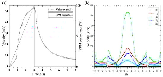
Figure 7. (a) Velocity variation with time at the central position (X = 5.3, y = 1.685, z = 0). (b) Wind speed curves at different times (t = 0, 1, 3, 5, 8 s) (y = 1.685, z = 0).

3.4. Wind Shear

In low-altitude urban environments, wind shear represents another impactful wind pattern. Wind shear is categorized into horizontal wind shear and vertical wind shear. For horizontal wind shear simulation, the configuration is as follows: from left to right, the rotational speed of the fans in the horizontal fixed fan wall decreases sequentially by 300 rpm from a maximum speed of 10,000 rpm. For vertical wind shear simulation, the configuration is as follows: from top to bottom, the rotational speed of the fans in the horizontal fixed fan wall decreases sequentially by 300 rpm from a maximum speed of 10,000 rpm.

Figure 8a,b present the fan rotational speed results, clearly showing that all fan speeds exhibit linear variation, consistent with the preset configurations. As shown in Figure 8c,d, which display the velocity contour maps of horizontal and vertical wind shear, both types of wind shear exhibit well-defined linear gradients and clear layering in the test section, with a shear magnitude from maximum to minimum of approximately 20 m/s. Furthermore, calculated results indicate that within the 10 m × 10 m test area, the linear correlation coefficient of the velocity profile R² > 0.98; affected by the end-wall effect, the gradient deviation in the edge region (within <1 m from the boundary) is about 12%. This demonstrates that the self-designed fan and the complex wind field simulation system can effectively simulate low-altitude wind shear; the dynamic similarity error of the generated shear flow field is below 10%, meeting the certification test requirements for aircraft; and it fills a technical gap in multi-directional dynamic shear simulation in traditional wind tunnels. In future work, real-time feedback control will be introduced to dynamically adjust the speed gradient to compensate for the wall effect, and temperature-humidity coupling will be incorporated to experimentally study the simulation of thermal vertical shear effects through superimposed temperature gradients.

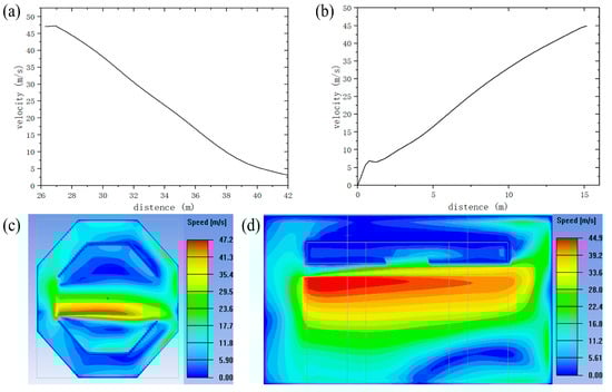
Figure 8. Wind Shear Contour Maps. (a) Horizontal wind shear velocity variation curve with position; (b) Vertical wind shear velocity variation curve with position; (c) Horizontal wind shear velocity contour map; (d) Vertical wind shear velocity contour map.

3.5. Tornado

Tornadoes represent a type of low-altitude wind field characterized by vertical motion in the simulation of complex low-altitude wind environments. In the numerical simulation of tornadoes, this study employed three distinct structural designs.

The first structural design for tornado simulation employs a configuration with three swirl fans installed along the long side of the bottom, two swirl fans along the short side, all oriented inward at a 45-degree angle, while four large fans at the top exhaust air outward. The swirl fans were operated at 1000 rpm. The corresponding results are presented in Figure 9.

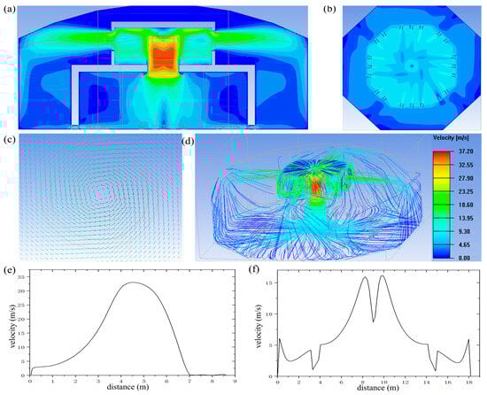
Figure 9. The first Tornado wind field contour maps. (a) Vertical direction velocity contour map; (b) Bottom swirl fan cross-sectional velocity contour map; (c) Velocity vector diagram; (d) Velocity streamline; (e) Vertical wind speed curve at central position; (f) Horizontal velocity at central position.

The second structural design employs six small fans on each side at the bottom, directed inward at a 10-degree angle, with one large fan on each side at the top configured for exhaust. This configuration transforms the pressure stabilization chamber from a rectangular to an octagonal prism. All swirl fans operate at 1000 rpm. The corresponding simulation results are shown in Figure 10.

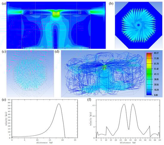
Figure 10. The second Tornado wind field contour maps. (a) Vertical direction velocity contour map; (b) Bottom swirl fan cross-sectional velocity contour map; (c) Velocity vector diagram; (d) Velocity streamline; (e) Vertical wind speed curve at central position; (f) Horizontal velocity at central position.

Figure 10a displays the velocity contour map in the Z-direction. The figure shows that the maximum wind speed occurs at the bell mouth below the pressure stabilization chamber, reaching approximately 50 m/s. The jet flow follows the vortex core contraction acceleration effect, after which the wind speed gradually decreases downward. In the lower test region, the central point exhibits low velocity (approximately 0 m/s), while the surrounding area shows higher velocities (around 10 m/s), consistent with the wind speed distribution characteristics of tornadoes. The test region exhibits a combined structure of forced vortex and free vortex, with detailed characteristics of the data curves provided in Figure 10e,f. Additionally, Figure 10b, which illustrates the velocity distribution contour of the bottom swirl fans, reveals that the flow at the bottom clearly exhibits rotational motion from the center to the periphery, in accordance with typical tornado wind speed patterns. The velocity vector diagram in Figure 10c further demonstrates the flow behavior of the simulated airflow, clearly showing the surrounding air converging spirally toward the center, consistent with logarithmic spiral trajectories. Figure 10d presents the velocity streamline diagram of this tornado simulation, from which the pathlines of the airflow are clearly visible: air flows spirally upward from the periphery toward the center, ultimately forming a tornado-like flow structure. These simulation results confirm that the complex wind field design can effectively generate specialized vertical wind fields and validate the design’s effectiveness and efficiency. As shown in Figure 9 and Figure 10, both structural designs are capable of forming tornado-like flows; however, the second design, with an octagonal pressure stabilization chamber, generates higher wind speeds. Compared to the rectangular prism structure, the octagonal geometry significantly mitigates the “corner flow” effect, resulting in a more uniform circumferential velocity distribution. In terms of core wind speed, it enhances the vorticity effect, and regarding turbulence characteristics, the octagonal configuration exhibits more stable flow behavior, more closely resembling the actual rotational characteristics of tornadoes.

3.6. Downburst

In addition to generating tornadoes in the vertical wind field, this design also simulates another common low-altitude wind pattern: the downburst. In the simulation modeling, four large fans installed at the top blow inward at a rotational speed of 1480 rpm, while small fans at the bottom exhaust outward at 300 rpm to replicate the downburst wind field environment. The simulation results are presented in Figure 11.

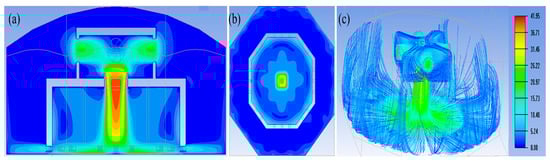
Figure 11. Downburst wind field contour maps. (a) Vertical velocity contour map; (b) Horizontal velocity contour map at central height; (c) Flow field streamline.

For the simulation of downbursts, following the impinging jet theory and wall jet principle in fluid mechanics, high-speed downward airflow is generated by four high-power fans at the top (1480 rpm), while the bottom exhaust system (300 rpm) produces radial outflow. As shown in the simulation results in Figure 11, the three-stage dynamic characteristics of downbursts are accurately reproduced.

As observed from the simulation results in Figure 11, the velocity distribution of the overall wind environment features downward flow from the circular bell mouth at the central top. The airflow impacts the ground and is then discharged radially from the inner cabin to the outer cabin. The converging airflow generated by the top fan cluster forms an axisymmetric circular jet, which is accelerated through the convergent bell mouth (Venturi effect), maintaining a typical downburst velocity magnitude of 40 m/s in the potential flow core region—consistent with the velocity decay behavior of axisymmetric jets governed by the Navier–Stokes equations. When the high-speed airflow impinges on the ground platform, stagnation pressure is generated. CFD simulation reveals a distinct pressure extreme zone (pressure coefficient Cp > 1.5), a phenomenon consistent with Hjelmfelt’s numerical simulation studies [42]. A strong shear layer develops near the ground (δ ≈ 0.1 D, where D is the jet diameter), leading to a sharp increase in turbulent kinetic energy (the k-ε model indicates a turbulence intensity exceeding 30%). The horizontal outflow formed after impact exhibits typical wall jet characteristics, with velocity profiles conforming to Glauert’s similarity solution and boundary layer development following the power-law relation δ∝x^0.8. The bottom annular exhaust system ensures outflow symmetry through mass flow control, and Reynolds stress measurements confirm that the anisotropic turbulence characteristics align with real microburst observation data.

The numerical simulation results demonstrate that in the dual-circuit air duct design, the primary circuit achieves energy conservation for macro-scale flow and maintains a steady wind field through the return-flow channel; the secondary circuit forms a local high-energy region via active jet control, with its velocity gradient ∇U ≈ 15 (m/s)/m matching precisely the internationally recognized downburst wind profile model. Simulation verification indicates that the radial wind speed decay exponent n = 1.28 ± 0.05, which aligns closely with the Oseguera–Bowles theoretical solution (n = 1.25). Through the simulation outcomes, this design overcomes the single-field simulation limitation of conventional wind tunnels. By implementing coordinated control of multi-stage fans, it achieves an adjustable parameter space encompassing an impinging jet Reynolds number of Re = 2.1 × 10⁵ (critical turbulent state) and a defined circulation ratio, thereby providing an experimental platform compliant with the ASCE/SEI 49-21 standard for research on coupled effects in extreme wind fields.

3.7. Special Wind Fields

3.7.1. Downward Turning Wind

The downward-turning wind represents a characteristic pattern in low-altitude urban wind fields, particularly around city buildings. To investigate the influence of outlet position on the simulation of such wind fields, this numerical simulation establishes two groups of outlet configurations for comparative analysis. The first group positions the outlet in the lower section of the area opposite the fan array, measuring 18.6 m × 3.8 m. The second group locates the outlet in the central-lower part of the same area, with dimensions of 10 m × 1.5 m. Figure 12 presents the velocity contours and vector diagrams for both outlet configurations.

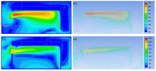
Figure 12. Downward turning wind field contour maps. (a) Velocity contour map of downward turning wind; (b) Velocity vector diagram of downward turning wind; (c) Velocity contour map of downward turning wind with modified outlet; (d) Velocity vector diagram of downward turning wind with modified outlet.

It can be clearly observed that the fan outlet velocity in the first configuration is significantly higher—approximately 4 m/s greater than that in the second. Moreover, in the second configuration, the wind speed drops sharply from a high value (36 m/s) to a low range (0–5 m/s) within a very short distance (2 m), resulting in a continuous scenario involving both gusts and wind shear, which poses substantial impacts on low-altitude drones. In the first configuration, the wind speed decreases linearly over a 20 m height range, exhibiting a lower level of wind shear. A comparison of the figures also reveals that the low-speed area (0–9 m/s) is larger in the second case, whereas only a small low-speed zone forms near the outlet in the first case.

These results indicate that by adjusting the outlet position, the turning radius of the downward-turning wind can be altered, and different degrees of vertical wind shear can be generated. This numerical simulation verifies the effectiveness and feasibility of designing such specialized wind fields.

3.7.2. Left-Right Turning Wind

For the optimization of the horizontal flow wind field, in addition to modifying the size of the self-developed fans, this numerical simulation study also optimized the outlet position by relocating it from the opposite side to the left and right sides, with the left and right sides of the opposite wall set as outlets for horizontal flow simulation while keeping other conditions unchanged. This type of wind field also represents a characteristic structure in low-altitude urban environments and is of great significance for studying the properties of low-altitude urban wind fields. The numerical simulation results are presented in Figure 13. As shown in Figure 13, the wind field velocity gradually increases from the fan outlet to a maximum value of 87 m/s, and the area of the maximum wind speed region is significantly larger compared to the configuration with the opposite side set as the outlet. In other words, this experimental setup for the horizontal flow field can, on one hand, expand the high-speed test area; on the other hand, in low-altitude urban settings where such building environments occur, the impact of large high-speed regions on drones must be considered.

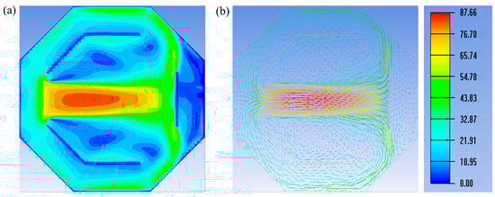
Figure 13. (a) Velocity contour map of left-right turning wind; (b) Velocity vector diagram of left-right turning wind.

3.7.3. Alley Wind

Alley wind is a highly common and readily formed wind field in low-altitude urban environments. To investigate whether the present design can effectively generate such characteristic urban wind fields, a numerical simulation was conducted to validate the design’s performance. In this simulation, two square structures were placed in the center of the test section to represent urban buildings, a low-altitude urban wind field was generated by fixed fan walls, and the fan outlet wind speed was set to 60 m/s. The numerical results are shown in Figure 14.

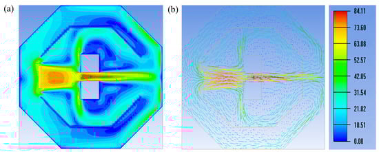
Figure 14. (a) Velocity contour map of alley wind; (b) Velocity vector diagram of alley wind.

The figure clearly reveals typical alley wind characteristics: the wind speed initially increases and then decreases along the path from the fan outlet toward the buildings. Notably, across a large area at the windward junction between the buildings and the wind field, the wind speed drops to approximately 30 m/s—half of the fan outlet speed. However, at the four corners where the buildings interface with the wind field, wind speeds are higher than at other positions along the junction surface. In particular, the two corners at the entrance of the alley formed by the buildings exhibit higher wind speeds than the other two corners.

The figure also clearly demonstrates that as the flow enters the alley between the buildings, the wind speed increases sharply and rapidly: it rises from 55 m/s at the alley entrance to 84 m/s within a 1 m distance. This high-speed region persists through the alley and extends downstream to a length approximately twice that of the alley itself. Furthermore, inside the alley, wind speed increases rapidly from the building surfaces toward the center: the velocity near the building surface is about 35 m/s and rises to 84 m/s within 1 m, consistent with one-dimensional compressible flow theory. After exiting the alley, the wind speed gradually decreases, forming a flame-like wake structure, which also represents a form of wind shear.

From the velocity vector diagram in Figure 14b, low-speed vortex structures can also be observed at the two leeward building corners not directly exposed to the incoming wind—a phenomenon that warrants attention. This numerical simulation effectively verifies the capability of the design to reproduce urban alley winds and provides in-depth theoretical insight into such flows, offering valid simulation-based theoretical support for subsequent experimental modeling.

3.7.4. Updraft and Downdraft Wind

In low-altitude urban environments, buildings constitute a common feature, and when wind flows around these structures, they can generate characteristic wind patterns known as updraft and downdraft flows. To verify the capability of this design to produce such specialized wind fields, the numerical simulation incorporated four distinct scenarios within the test area for simulation and optimization analysis. The first scenario featured a 16 m-high building within the test area, with only a 2 m gap above the structure to facilitate observation of flow field distribution. Figure 15a,b present the velocity contour map and vector diagram corresponding to this numerical analysis.

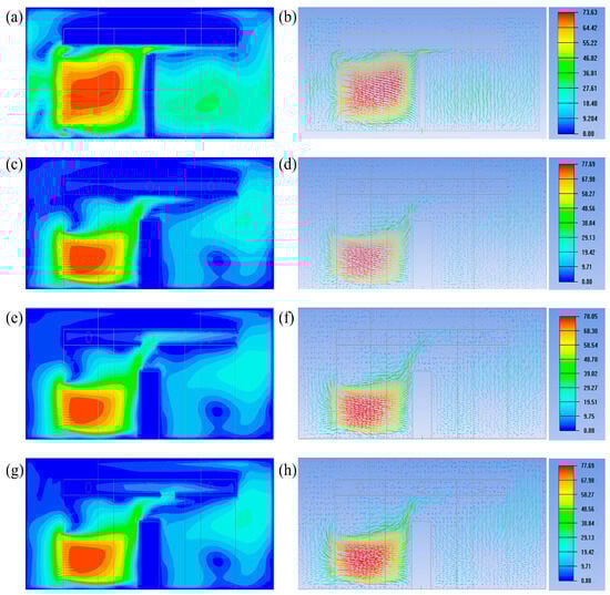
Figure 15. Updraft and downdraft wind field contour maps. (a) Velocity contour map of updraft and downdraft flows; (b) Velocity vector diagram of updraft and downdraft flows; (c) Velocity contour map with closed top bellmouth; (d) Velocity vector diagram with closed top bellmouth; (e) Velocity contour map with open top bellmouth; (f) Velocity vector diagram with open top bellmouth; (g) Velocity contour map with rectangular top opening; (h) Velocity vector diagram with rectangular top opening.

The figures reveal that the excessively tall obstructing building resulted in poorly defined updraft and downdraft flows. Consequently, an optimized model was developed by modifying the obstruction dimensions to 13 m in height and 16 m in width, while closing the bellmouth. The corresponding simulation results are presented in Figure 15c,d. These results demonstrate that reducing the building height amplifies the velocity differential, making both updraft and downdraft flows significantly more pronounced. To further investigate the influence of top opening configuration on these flow patterns, comparative simulations were performed by alternately opening the top circular bellmouth and redesigning it with a rectangular geometry. The simulation results for these configurations are shown in Figure 15e–h.

Comparison between Figure 15e,f indicates that opening the top bellmouth results in a gentler wind speed gradient and increased wind velocity at the building’s downward corners, reflecting an acceleration of downdraft flow at the rooftop while producing relatively minor changes in other regions. This suggests that while the top opening condition influences the initiation of downdraft flows, its subsequent effects remain limited. Similarly, comparison between Figure 15g,h reveals that changing the bellmouth shape from circular to rectangular also significantly alters the downdraft behavior at the top. Through these simulations of four distinct structural configurations, it is established that modifying the top structure can effectively modulate updraft and downdraft characteristics. This finding will form the basis for subsequent simulation optimization and experimental investigations, while simultaneously verifying the capability of this design to effectively simulate the specialized low-altitude wind fields of updraft and downdraft flows.

3.7.5. Crossroads Wind

Crossroads wind represents a variant form of alley wind in low-altitude urban environments. In this numerical simulation, the two fan walls were configured vertically to simulate two distinct scenarios: one in which the converging crossroads wind encounters no downstream building obstruction, and another in which building obstruction is present after convergence. The numerical simulation results are presented in Figure 16.

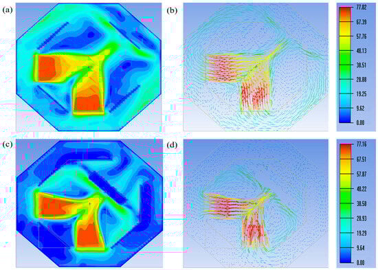
Figure 16. Crossroads Wind Field Contour Maps. (a) Crossroads wind velocity contour map; (b) Crossroads wind velocity vector diagram; (c) Top-view velocity contour map of crossroads wind with obstructions; (d) Top-view velocity vector diagram of crossroads wind with obstructions.

As observed in Figure 16a,b, in the unobstructed case, the two independently generated wind fields converge at an angle of approximately 45 degrees. At the initial interface of convergence, the wind speed decreases sharply from high to low, with a localized region of near-zero velocity—indicating significant wind shear occurring over a small spatial scale. Along the 45-degree diagonal from this interface, the wind speed initially increases and then decreases, exhibiting a flame-shaped distribution, with the maximum value located at the intersection of the far cross-sections of the two fan walls. This simulation reveals that after convergence of two vertically aligned crossroad wind flows, an oblique wind shear layer develops; that is, vertically incoming flows form a stable inclined shear layer in an open environment.

When the converged wind field encounters building obstructions, as shown in Figure 16c,d, the buildings significantly alter the flow structure. In particular, the outer regions of both wind streams are compressed inward, resulting in an arc-shaped flow pattern rather than the linear configuration observed in the unobstructed case. Additionally, after reaching its maximum, the wind speed decreases rapidly post-convergence, as the building corners induce a Dual Vortex System that deflects the outer airflow inward. These results indicate that although low-altitude crossroads wind exhibits different characteristics under obstructed and unobstructed conditions, in both cases an oblique shear layer forms along the convergence direction. This numerical study also verifies the effectiveness of the proposed design in simulating crossroads wind environments.

4. Conclusions

Against the background of the low-altitude economy and the testing requirements of new aircraft such as unmanned aerial vehicles (UAVs) and flying cars in complex urban wind field environments, this study designed and validated a low-altitude complex wind field simulation device with multi-physics coupling capability. By integrating theoretical analysis, numerical simulation, and experimental verification, the research systematically investigated simulation methods for horizontal flows, vertical flows, and various special wind fields (including gusts, wind shear, tornadoes, and downbursts), and provided an in-depth exploration of the formation mechanisms of typical urban wind fields (such as alley winds, crossroads winds, updrafts, and downdrafts).

Numerical simulation results demonstrate that the proposed multi-fan coordinated control scheme can effectively simulate low-altitude complex wind field environments. In the optimized horizontal flow wind field, the wind speed reaches 83 m/s within the test section, with turbulence intensity ranging from 5% to 20%. The gust simulation achieves a wind speed increase from 0 to 53 m/s within 3 s, followed by a decay to 5 m/s within 5 s after shutdown. Through linear regulation of fan speeds, the wind shear simulation realizes stratified shear of 20 m/s in both horizontal and vertical directions, providing a reliable environment for aircraft wind shear resistance testing. Furthermore, by coordinating the operation of bottom swirl fans and top exhaust systems, extreme wind fields such as tornadoes (with a central spiral wind speed of 50 m/s) and downbursts (with a downward central vertical jet velocity of 40 m/s) are successfully reproduced, laying a foundation for evaluating aircraft performance under adverse weather conditions.

Simulation analysis of typical urban wind fields reveals the substantial impact of building configurations on wind field behavior. Alley wind simulations demonstrate that as the flow passes through a narrow passage, the wind speed increases sharply from 55 m/s to 84 m/s within a 1 m distance, while distinct vortex structures form on the leeward side of buildings. Crossroads wind simulations indicate that when two perpendicular wind fields converge, oblique wind shear develops; the presence of building obstructions further modifies the flow distribution, generating complex turbulent structures. These findings offer valuable insights for path planning and disturbance-rejection control of aircraft operating in urban environments.

The innovations of this study are as follows: it proposes a low-altitude wind tunnel design capable of simulating multi-directionally coupled wind fields; achieves full active control of the Reynolds stress tensor; overcomes the limitation of conventional wind tunnels in generating only uniform laminar flow; and fills the technical gap in simulation facilities for low-altitude complex wind fields. By leveraging nonlinear coupling of jet interactions, the energy spectrum characteristics of urban wind fields are accurately reproduced. At the same time, this study provides fundamental wind field data to support the development of low-altitude complex environment simulation devices that integrate complex wind fields with environmental factors such as high temperature, low temperature, humidity, rain, and wind-driven rain—content that will form the basis for our team’s future research and design. The completed installation is shown in Figure 17, with further detailed testing and validation experiments to be conducted in Shensi Lab in Shenzhen.

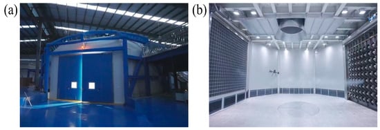
Figure 17. (a) Structural Diagram of the Device, (b) Flight Test Status Diagram.

In the future, this technology can be further extended to aerodynamic optimization of aircraft, urban wind environment assessment, and the formulation of low-altitude traffic management standards, offering valuable references for understanding the characteristics of low-altitude complex wind fields and supporting related research in the low-altitude economy. Follow-up research will focus on optimizing dynamic wind field control algorithms and testing the performance of physical aircraft in simulated wind fields to advance the engineering application of this technology. It is anticipated that this facility could serve as a useful platform bridging fundamental turbulence research and low-altitude engineering applications, providing a reference for future developments in “digital twin-driven high-precision experiments” in fluid mechanics.

References

- Wang, L.; Yang, Z.; Gu, X.; Li, J. Linkages Between Tropical Cyclones and Extreme Precipitation over China and the Role of ENSO. Int. J. Disaster Risk Sci. 2020, 11, 538–553. [Google Scholar] [CrossRef]
- Nayak, S.; Takemi, T. Typhoon-induced precipitation characterization over northern Japan: A case study for typhoons in 2016. Prog. Earth Planet. Sci. 2020, 7, 39. [Google Scholar] [CrossRef]
- Cherubini, A.; Papini, A.; Vertechy, R.; Fontana, M. Airborne Wind Energy Systems: A review of the technologies. Renew. Sustain. Energy Rev. 2015, 51, 1461–1476. [Google Scholar] [CrossRef]
- Weber, J.; Marquis, M.; Lemke, A.; Cooperman, A.; Draxl, C.; Lopez, A.; Roberts, O.; Shields, M. Proceedings of the 2021 Airborne Wind Energy Workshop; National Renewable Energy Lab. (NREL): Golden, CO, USA, 2021. [Google Scholar]
- Blocken, B.; Stathopoulos, T.; van Beeck, J.P.A.J. Pedestrian-level wind conditions around buildings: Review of wind-tunnel and CFD techniques and their accuracy for wind comfort assessment. Build. Environ. 2016, 100, 50–81. [Google Scholar] [CrossRef]
- Stull, R.B. An Introduction to Boundary Layer Meteorology; Springer: Berlin/Heidelberg, Germany, 1988. [Google Scholar]
- Barlow, J.F.; Halios, C.H.; Lane, S.E.; Wood, C.R. Observations of urban boundary layer structure during a strong urban heat island event. Environ. Fluid Mech. 2014, 15, 373–398. [Google Scholar] [CrossRef]
- Stamate, M.A.; Pupaza, C.; Nicolescu, F.A.; Moldoveanu, C.E. Improvement of Hexacopter UAVs Attitude Parameters Employing Control and Decision Support Systems. Sensors 2023, 23, 1446. [Google Scholar] [CrossRef]
- Wing, D.J.; Chancey, E.T.; Politowicz, M.S.; Ballin, M.G. Achieving resilient in-flight performance for advanced air mobility through simplified vehicle operations. In Proceedings of the AIAA Aviation 2020 Forum, Reno, NV, USA, 15–19 June 2020; p. 2915. [Google Scholar]
- Basawanal, A. Development and Qualification of a Drone-Based Anemometry Platform for Air Risk Assessment in Urban Environments. Ph.D. Thesis, Carleton University, Ottawa, ON, Canada, 2024. [Google Scholar]
- Giersch, S.; El Guernaoui, O.; Raasch, S.; Sauer, M.; Palomar, M. Atmospheric flow simulation strategies to assess turbulent wind conditions for safe drone operations in urban environments. J. Wind. Eng. Ind. Aerodyn. 2022, 229, 105136. [Google Scholar] [CrossRef]
- Raza, S.A. Autonomous UAV Control for Low-Altitude Flight in an Urban Gust Environment. Ph.D. Thesis, Carleton University, Ottawa, ON, Canada, 2015. [Google Scholar]
- Cobano, J.A.; Alejo, D.; Sukkarieh, S.; Heredia, G.; Ollero, A. Thermal detection and generation of collision-free trajectories for cooperative soaring UAVs. In Proceedings of the 2013 IEEE/RSJ International Conference on Intelligent Robots and Systems, Tokyo, Japan, 3–7 November 2013; pp. 2948–2954. [Google Scholar]
- Chakrabarty, A.; Langelaan, J.W. Energy-Based Long-Range Path Planning for Soaring-Capable Unmanned Aerial Vehicles. J. Guid. Control Dyn. 2011, 34, 1002–1015. [Google Scholar] [CrossRef]
- Boyet, G. ESWIRP: European Strategic Wind tunnels Improved Research Potential program overview. CEAS Aeronaut. J. 2018, 9, 249–268. [Google Scholar] [CrossRef]
- Holthusen, H.; Bergmann, A.; Sijtsma, P. Investigations and measures to improve the acoustic characteristics of the German-Dutch Wind Tunnel DNW-LLF. In Proceedings of the 18th AIAA/CEAS Aeroacoustics Conference (33rd AIAA Aeroacoustics Conference), Springs, CO, USA, 4–6 June 2012; p. 2176. [Google Scholar]
- Carlino, G.; Cardano, D.; Cogotti, A. A New Technique to Measure the Aerodynamic Response of Passenger Cars by a Continuous Flow Yawing; SAE Technical Paper 0148-7191; SAE International: Warrendale, PA, USA, 2007. [Google Scholar]
- Shams, T.A.; Shah, S.I.A.; Ahmad, M.A. Capability analysis of global hypersonic wind tunnel facilities for aerothermodynamic investigations. In Proceedings of the 2020 17th International Bhurban Conference on Applied Sciences and Technology (IBCAST), Islamabad, Pakistan, 14–18 January 2020; pp. 481–501. [Google Scholar]
- Lee, T.; Lin, G. Review of experimental investigations of wings in ground effect at low Reynolds numbers. Front. Aerosp. Eng. 2022, 1, 975158. [Google Scholar] [CrossRef]
- Greenwood, W.W.; Lynch, J.P.; Zekkos, D. Applications of UAVs in Civil Infrastructure. J. Infrastruct. Syst. 2019, 25, 04019002. [Google Scholar] [CrossRef]
- Moshref-Javadi, M.; Winkenbach, M. Applications and Research avenues for drone-based models in logistics: A classification and review. Expert Syst. Appl. 2021, 177, 114854. [Google Scholar] [CrossRef]
- Lee, D.; Yee, K. Novel Electric Propulsion System Analysis Method for Electric Vertical Takeoff and Landing Aircraft Conceptual Design. J. Aircr. 2024, 61, 375–391. [Google Scholar] [CrossRef]
- Ehirim, O.H.; Knowles, K.; Saddington, A.J. A Review of Ground-Effect Diffuser Aerodynamics. J. Fluids Eng. 2019, 141, 020801. [Google Scholar] [CrossRef]
- Zhang, X.; Zerihan, J. Off-surface aerodynamic measurements of a wing in ground effect. J. Aircr. 2003, 40, 716–725. [Google Scholar] [CrossRef]
- Talavera, M.; Shu, F. Experimental study of turbulence intensity influence on wind turbine performance and wake recovery in a low-speed wind tunnel. Renew. Energy 2017, 109, 363–371. [Google Scholar] [CrossRef]
- Flay, R.G.J. A twisted flow wind tunnel for testing yacht sails. J. Wind Eng. Ind. Aerodyn. 1996, 63, 171–182. [Google Scholar] [CrossRef]
- Tse, K.T.; Weerasuriya, A.U.; Kwok, K.C.S. Simulation of twisted wind flows in a boundary layer wind tunnel for pedestrian-level wind tunnel tests. J. Wind Eng. Ind. Aerodyn. 2016, 159, 99–109. [Google Scholar] [CrossRef]
- Hangan, H. The wind engineering energy and environment (WindEEE) Dome at Western University, Canada. Wind Eng. JAWE 2014, 39, 350–351. [Google Scholar] [CrossRef]
- Blocken, B. Computational Fluid Dynamics for urban physics: Importance, scales, possibilities, limitations and ten tips and tricks towards accurate and reliable simulations. Build. Environ. 2015, 91, 219–245. [Google Scholar] [CrossRef]
- Tennekes, H.; Lumley, J.L. A First Course in Turbulence; MIT press: Cambridge, MA, USA, 1972. [Google Scholar]
- Stull, R.B. An Introduction to Boundary Layer Meteorology; Springer Science & Business Media: Berlin/Heidelberg, Germany, 2012; Volume 13. [Google Scholar]
- Ferziger, J.H.; Perić, M. Computational Methods for Fluid Dynamics; Springer: Berlin/Heidelberg, Germany, 2002; Volume 586. [Google Scholar]
- Versteeg, H.K. An Introduction to Computational Fluid Dynamics the Finite Volume Method, 2nd ed.; Pearson Education India: Bangalore, India, 2007. [Google Scholar]
- Launder, B.E.; Spalding, D.B. The Numerical Computation of Turbulent Flows. In Numerical Prediction of Flow, Heat Transfer, Turbulence and Combustion; Elsevier: Amsterdam, The Netherlands, 1983; pp. 96–116. [Google Scholar]
- Menter, F.R. Two-equation eddy-viscosity turbulence models for engineering applications. AIAA J. 1994, 32, 1598–1605. [Google Scholar] [CrossRef]
- Reynolds, O. IV. On the dynamical theory of incompressible viscous fluids and the determination of the criterion. Philos. Trans. R. Soc. Lond 1997, 186, 123–164. [Google Scholar] [CrossRef]
- Wilcox, D.C. Turbulence Modeling for CFD; DCW industries: La Canada, CA, USA, 1998; Volume 2. [Google Scholar]
- Spalart, P.R. Strategies for turbulence modelling and simulations. Int. J. Heat Fluid Flow 2000, 21, 252–263. [Google Scholar] [CrossRef]
- Kundu, P.K.; Cohen, I.; Dowling, D.R. Fluid Mechanics; Academic Press: Cambridge, MA, USA, 1990. [Google Scholar]
- Rodi, W. Experience with two-layer models combining the k-epsilon model with a one-equation model near the wall. In Proceedings of the 29th Aerospace Sciences Meeting, Reno, NV, USA, 7–10 January 1991; p. 216. [Google Scholar]
- Tominaga, Y.; Mochida, A.; Yoshie, R.; Kataoka, H.; Nozu, T.; Yoshikawa, M.; Shirasawa, T. AIJ guidelines for practical applications of CFD to pedestrian wind environment around buildings. J. Wind. Eng. Ind. Aerodyn. 2008, 96, 1749–1761. [Google Scholar] [CrossRef]
- Hjelmfelt, M.R. Structure and life cycle of microburst outflows observed in Colorado. J. Appl. Meteorol. Climatol. 1988, 27, 900–927. [Google Scholar] [CrossRef]
Disclaimer/Publisher’s Note: The statements, opinions and data contained in all publications are solely those of the individual author(s) and contributor(s) and not of MDPI and/or the editor(s). MDPI and/or the editor(s) disclaim responsibility for any injury to people or property resulting from any ideas, methods, instructions or products referred to in the content. |
© 2025 by the authors. Licensee MDPI, Basel, Switzerland. This article is an open access article distributed under the terms and conditions of the Creative Commons Attribution (CC BY) license (https://creativecommons.org/licenses/by/4.0/).