Abstract
Accurate short- and medium-term forecasting of photovoltaic (PV) power generation is vital for grid stability and renewable energy integration. This study presents a comparative scenario-based approach using Long Short-Term Memory (LSTM), Convolutional Neural Network (CNN), and Gated Recurrent Unit (GRU) models trained with one year of real-time meteorological and production data from a 250 kWp grid-connected PV system located at Dicle University in Diyarbakır, Southeastern Anatolia, Turkey. The dataset includes hourly measurements of solar irradiance (average annual GHI 5.4 kWh/m2/day), ambient temperature, humidity, and wind speed, with missing data below 2% after preprocessing. Six forecasting scenarios were designed for different horizons (6 h to 1 month). Results indicate that the LSTM model achieved the best performance in short-term scenarios, reaching R2 values above 0.90 and lower MAE and RMSE compared to CNN and GRU. The GRU model showed similar accuracy with faster training time, while CNN produced higher errors due to the dominant temporal nature of PV output. These results align with recent studies that emphasize selecting suitable deep learning architectures for time-series energy forecasting. This work highlights the benefit of integrating real local meteorological data with deep learning models in a scenario-based design and provides practical insights for regional grid operators and energy planners to reduce production uncertainty. Future studies can improve forecast reliability by testing hybrid models and implementing real-time adaptive training strategies to better handle extreme weather fluctuations.
1. Introduction
The growing global population, rapidly advancing technologies, and the consequent continuous rise in energy demand are intensifying the dependency on energy resources with each passing day. In particular, while the adverse impacts of the COVID-19 pandemic have not yet been fully overcome, Russia’s invasion of Ukraine has triggered a new global energy crisis, leading to a contraction in fossil fuel supply and subsequent price increases [1,2]. These developments have once again highlighted the economic and geopolitical vulnerabilities caused by excessive reliance on fossil fuel sources. Current projections indicate that global energy consumption is expected to increase by approximately 40% by 2040 [3]. This situation necessitates the replacement of environmentally harmful and finite fossil fuels with sustainable and clean energy sources. In response, many countries have announced carbon neutrality targets as part of their efforts to combat climate change, accelerating the transition to renewable energy sources and developing various incentive mechanisms [4].
The growing global demand for clean and sustainable energy has significantly accelerated the integration of renewable energy sources—particularly solar photovoltaic (PV) systems—into existing power grids. According to the International Energy Agency (IEA), solar PV systems have become the fastest-growing renewable energy technology worldwide in recent years, achieving record capacity additions [5,6]. The IEA’s Renewables 2022 report highlights a substantial increase in global solar PV investments, with installed PV capacity expected to grow by approximately 1500 GW by 2027, surpassing the capacity of coal-fired power plants [7]. However, due to its inherent nature, solar energy is highly influenced by meteorological factors such as solar irradiance, cloud cover, temperature, and humidity, which results in intermittency and variability—posing major challenges for grid stability and energy management [8,9]. To mitigate these uncertainties and ensure the efficient planning and operation of power systems, accurate forecasting of solar energy generation is essential. Solar forecasting methods are generally categorized into physical models, statistical models, machine learning-based approaches, and hybrid frameworks [10].
In addition to the comparative analysis provided in Table 1, recent advancements in Artificial Intelligence (AI) and Deep Learning (DL) techniques have demonstrated significant improvements in forecasting accuracy. Cutting-edge methods such as Long Short-Term Memory (LSTM) networks, Convolutional Neural Networks (CNNs), and Transformer-based architectures effectively model complex temporal dependencies and extract spatial features from multimodal inputs [11,12]. Recent studies have further emphasized the importance of advanced deep learning frameworks in enhancing forecast robustness under varying conditions [13]. For example, hybrid frameworks that combine CNN and LSTM layers outperform traditional models in both intra-hour and day-ahead forecasting tasks [14,15]. Moreover, Graph Neural Networks (GNNs) and attention-based architectures further enhance spatiotemporal feature learning, particularly in multi-site PV forecasting scenarios [16,17]. Another emerging trend is probabilistic forecasting, which quantitatively estimates forecast uncertainty and supports risk-aware grid operation and energy trading. Methods based on quantile regression, Gaussian processes, and advanced probabilistic Transformer models have made notable contributions to this domain [18,19].
Table 1.
Comparison of Deep Learning-Based PV Forecasting Studies.
Despite these advancements, current models still face limitations related to local weather variability, data availability, and region-specific conditions. Therefore, short- and medium-term forecasting of photovoltaic (PV) power generation has become a critical issue for ensuring grid stability and integrating renewable energy sources. In their 2023 study, Visser et al. emphasized the value of physics-based expert variables in forecasting models and proposed hybrid approaches [25]. Sun et al. developed CNN-based models to address uncertainties caused by cloud movement, aiming to improve short-term PV output forecasting [26]. Wang et al. enhanced prediction accuracy by optimizing a Bi-LSTM network using hybrid algorithms [27]. Suanpang and Jamjuntr highlighted the advantages of machine learning-based methods by comparing LGBM and KNN models for microgrid applications [28]. Perera et al. proposed a hierarchical convolutional neural network approach to accurately estimate the total output of rooftop PV systems across different climate zones on a regional basis [29]. Song et al. integrated NGBoost with attention-based neural networks to reduce uncertainty in ultra-short-term forecasting [30]. Hu et al. introduced a satellite-based hybrid method that combines cloud transmissivity and clear-sky radiation, significantly improving short-term GHI forecasting accuracy [31]. Mauladdawilah et al. [32] demonstrated that systematic meteorological variable selection significantly enhances PV forecasting performance. Their LSTM-based framework achieved 99.81% accuracy using only two satellite-derived inputs, showing that variable selection can be more critical than model complexity in PV prediction tasks [32]. Paolo et al. [33] comprehensively examined deep learning-based PV power forecasting methods developed based on weather data. The study compares different deep network architectures, including LSTM, GRU, CNN, and hybrid models, and analyzes the impact of meteorological variables (temperature, radiation, humidity, wind speed, etc.) on forecasting performance [33]. Palm et al. [34] developed and compared RNN, LSTM, GRU, and hybrid LSTM–GRU models for short-term PV power forecasting at the 30 MW Nagréongo solar plant in Burkina Faso. Their results showed that deep learning models, particularly LSTM and GRU, achieved high accuracy (nRMSE ≈ 2–5%) and strong adaptability under varying climatic conditions [34]. Cican et al. [35] compared LSTM and CNN architectures for hourly photovoltaic energy forecasting in Romania using real meteorological and production data. Their results showed that CNN models achieved superior accuracy (R2 = 0.9913, MAE = 9.74) and faster convergence than LSTMs, demonstrating strong generalization and robustness for short-term PV integration into the national grid [35]. Song et al. proposed a Flexible Hybrid Ensemble (FHE) framework that dynamically selects the most suitable base models (RF, SVR, LightGBM, XGBoost, Transformer, MLP) using a meta-model trained on historical error patterns for photovoltaic power forecasting [36]. Joo et al. compared LSTM and Echo State Network (ESN) models for time-series prediction of solar power generation, emphasizing optimized ESN hyperparameters such as spectral radius, input noise, and leakage rate [37].
Finally, Massidda et al. conducted a comparative analysis of probabilistic methods and physical-statistical models, contributing to improved uncertainty management in solar forecasting [38]. Collectively, these studies demonstrate that deep learning-based and hybrid approaches offer promising improvements in PV power forecasting performance.
This study aims to develop multiple deep learning models for short- and medium-term photovoltaic (PV) output forecasting in the Southeastern Anatolia region. By leveraging real-time meteorological data and advanced artificial intelligence techniques, the research seeks to enhance forecasting reliability and support efficient energy management and grid stability.
1.1. Study Motivation
The rapid expansion of photovoltaic (PV) power systems worldwide has increased the need for accurate and reliable forecasting methods to ensure grid stability and efficient energy management. While numerous studies have demonstrated the potential of machine learning and deep learning models in solar power prediction, many rely on simulated or limited-duration datasets that may not fully represent real operational conditions. Moreover, the performance of different deep learning architectures can vary significantly depending on regional climatic factors and the quality of local meteorological inputs.
Southeastern Anatolia, where the case study is located, has one of Turkey’s highest solar energy potentials, yet there is a lack of scenario-based comparative studies that integrate long-term field measurements with advanced forecasting models. By addressing this gap, this study aims to provide a practical, data-driven solution for grid operators and energy planners in regions with high solar variability. The use of real-time site-specific data combined with a comparative analysis of LSTM, CNN, and GRU models highlights the significance of selecting suitable architectures for different forecasting horizons and local conditions. This motivation aligns with the broader goal of supporting more reliable renewable energy integration and reducing uncertainty in solar power generation.
1.2. Case Study Contribution
Accurate forecasting of photovoltaic (PV) power output is becoming increasingly critical for maintaining grid stability and maximizing the efficiency of renewable energy integration, especially in regions with highly variable meteorological conditions. While recent studies have explored machine learning and deep learning approaches, many rely on limited or simulated datasets, reducing their practical applicability. This study addresses this gap by providing a real-field, scenario-based comparison of advanced deep learning models. The unique aspects and main contributions of this research are summarized below:
- This study establishes the first comprehensive deep learning forecasting benchmark for Southeastern Anatolia, a region characterized by high solar potential yet high meteorological volatility. Unlike studies relying on simulated data, this work utilizes high-resolution field data to validate model robustness against specific regional climatic stressors.
- Rather than a generic performance evaluation, the proposed framework designs six distinct forecasting scenarios (ranging from 1-h to 1-month horizons) to systematically stress-test the temporal generalization capabilities of Recurrent (LSTM, GRU) versus Convolutional (CNN) architectures under varying observational windows.
- The study provides empirical evidence demonstrating the superior adaptability of localized LSTM models over CNNs for medium-term horizons in this specific geographical context, offering a validated roadmap for grid operators in similar semi-arid climate zones.
2. Materials and Methods
2.1. System Description
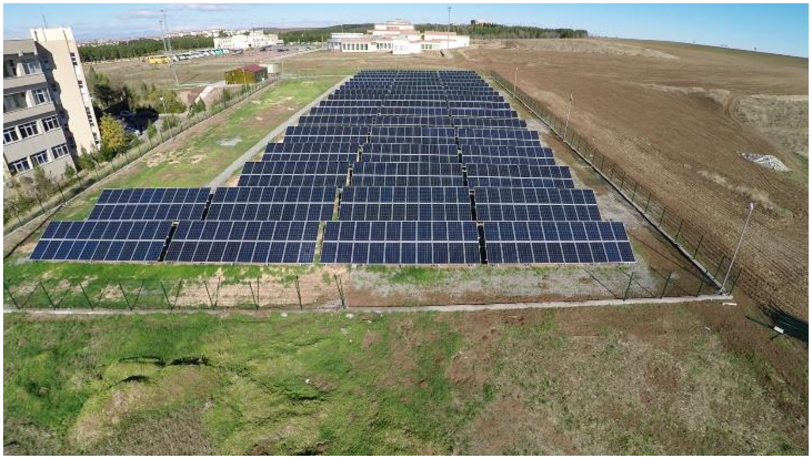
The Dicle University’s Solar Power Plant (DUSPP) is located at coordinates 40°16′ E longitude and 37°54′ N latitude, with a total installed capacity of 250 kWp. The plant comprises 1000 photovoltaic (PV) panels, each with a nominal capacity of 250 Wp, mounted southward at a tilt angle of 30°. Each module contains 60 solar cells, and the average nominal power obtained from actual measurements slightly exceeds the standard reference value, reaching 253.14 W [39]. An overview of the facility is provided in Figure 1.
Figure 1.
Dicle University’s Solar Power Plant (DUSPP).
The system is designed with eight strings, each rated at 30 kW, and one additional string rated at 10 kW. Each 30 kW string consists of six sub-arrays (arrays), where every three sub-arrays are connected to a separate maximum power point tracking (MPPT) input of an inverter. In contrast, the 10 kW string includes two sub-arrays, each connected to a separate MPPT input of its inverter. Each sub-array is configured with 20 panels connected in series.
The solar monitoring station installed on the roof of the Dicle University Science and Technology Research and Application Center (DÜBTAM) is utilized to meet the need for meteorological data [40]. The station performs essential measurements including global solar radiation, sunshine duration, air temperature, relative humidity, wind speed, and wind direction. To monitor these parameters, temperature and wind sensors are used alongside a pyranometer, and the collected data are recorded at 10-min intervals. All recorded data are transferred to a computer using Fimer-Aurora Vision 3.19 version software and organized for further analysis.
The meteorological dataset used in this study was collected directly from the DÜBTAM observation station located on the Dicle University campus. All measurements were recorded at 10-min intervals using calibrated pyranometer, temperature, humidity, and wind sensors. After quality control and removal of hardware-induced anomalies, the dataset was aggregated into hourly values for model training. A detailed statistical summary of all variables is presented in Section 2.2. Prior to model training, a rigorous preprocessing pipeline was applied. Although missing data accounted for less than 2% of the dataset, these gaps were filled using linear interpolation to preserve the local continuity of the meteorological trends. Subsequently, data normalization was performed to accelerate model convergence. All input features were scaled to the range [0, 1] using Min-Max Normalization. Crucially, to prevent data leakage, the minimum and maximum scaling parameters were calculated solely from the training set, and these parameters were then applied to transform the validation and test sets.
2.2. Data Statistical Analysis
The descriptive statistics presented in Table 2 provide an initial understanding of the distributional properties of the meteorological variables and PV power output used in this study. The PV power values range from 0 to 250,194 W, with a mean of 81,130 W and a relatively large standard deviation (74,044 W), reflecting the inherent variability of solar production due to diurnal cycles and weather fluctuations. The slight positive skewness (0.374) indicates that higher power values occur less frequently but extend the upper tail of the distribution, while the negative kurtosis (−1.377) suggests a flatter-than-normal distribution.
Table 2.
Descriptive Statistics of Meteorological and PV Power Variables.
Solar radiation exhibits similar distributional characteristics, with a mean of 430.6 W/m2 and a maximum of 1115 W/m2. The low skewness (0.187) and moderately negative kurtosis (−1.195) indicate a distribution that is close to symmetric but slightly platykurtic due to the contrast between nighttime zeros and daytime peaks. Ambient temperature ranges from −16.14 °C to 43.08 °C, showing the broad seasonal variation of the region. Its near-zero skewness (−0.112) suggests symmetry around the mean (19.95 °C), while the negative kurtosis (−0.941) reflects a relatively uniform spread of observations. Wind speed has a lower mean value (1.84 m/s) and moderate variability (std = 1.582 m/s). The positive skewness (1.033) indicates that low wind speeds are much more frequent than high speeds, while the slightly positive kurtosis (0.588) shows a distribution sharper than the normal distribution. Collectively, these descriptive statistics confirm that the dataset demonstrates realistic meteorological variability, which is essential for robust model training. The presence of skewness and platykurtic tendencies in several variables highlights the importance of proper normalization and model selection for capturing nonlinear relationships in PV power forecasting.
2.3. LSTM Model
Machine learning is the scientific study of extracting meaningful information from large datasets, recognizing patterns, and predicting future events [41]. In this study, Long Short-Term Memory (LSTM) networks are preferred, especially for time series analysis and energy production forecasting [42].
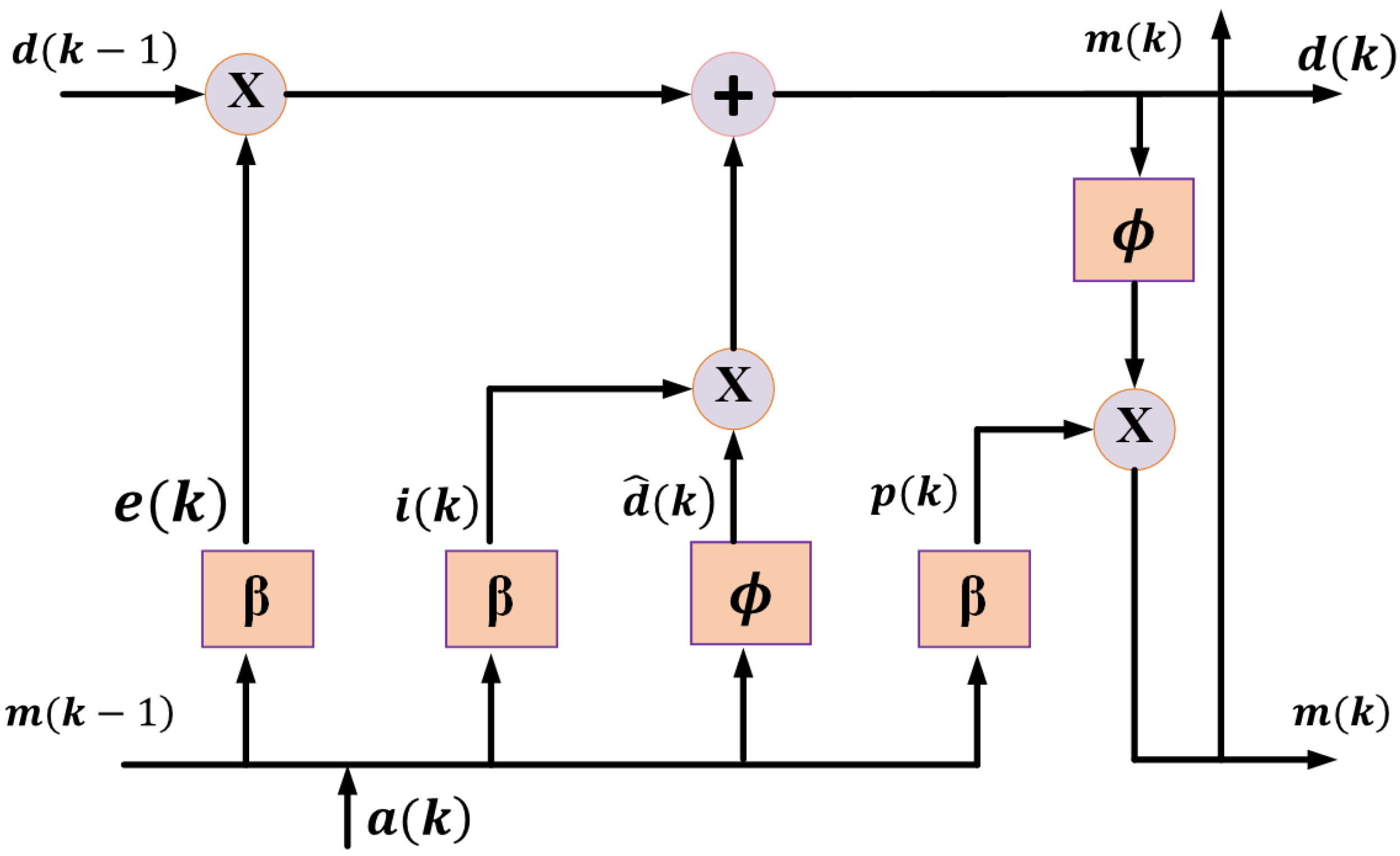
The most prevalent type of recurrent neural network (RNN) architecture is the LSTM, which comprises specialized structures known as memory blocks with gates [43,44]. Each LSTM unit includes a forget gate, an input gate, and an output gate, where these gates regulate the internal cell states [45,46]. The development of the LSTM architecture was pioneered by Hochreiter and Schmidhuber. The structural representation of the LSTM model, as depicted in Figure 2, illustrates its capacity to learn long-term dependencies within sequential time series data [47].
Figure 2.
LSTM model structure.
In a classical LSTM structure, the network consists of an input layer, one or more hidden layers, and an output layer. Later, a forget gate was introduced by Gers et al. [48]. The input sequence is denoted as , where represents the feature vector at time step k. A memory block comprising L memory cells and an input feature vector is updated H times—once for each feature vector in the input array.
At each update step, the current state vector is , while represents the previous cell state. The cell output vector is , and the prior output vector is . Input activation vector , forget activation vector , and output activation vector are computed at each time step using the sigmoid activation function , while the hyperbolic tangent function is used for candidate cell states.
The mathematical representation of an LSTM unit is given as follows:
Here, ⊙ denotes element-wise multiplication, W and U are weight matrices, and b represents bias vectors.
The LSTM architecture is capable of capturing both short-term and long-term temporal dependencies. Consequently, LSTM models serve as a powerful tool in applications where historical data are critical for future prediction, such as photovoltaic power generation forecasting.
2.4. CNN Model
Convolutional Neural Networks (CNNs), typically used for image processing, are adapted here for time-series forecasting using 1D convolution layers. The model extracts local temporal features from the multivariate input sequence. The convolution operation is defined as:
where W is the filter kernel, is the input vector, and b is the bias. Our architecture utilizes a 1D-CNN layer followed by a Max-Pooling layer to down-sample the features before feeding them into fully connected layers.
2.5. GRU Model
The Gated Recurrent Unit (GRU) is a streamlined variant of the LSTM that merges the forget and input gates into a single update gate. This reduces computational complexity while maintaining the ability to capture long-term dependencies. The hidden state is computed as follows:
2.6. Experimental Setup and Data Partitioning
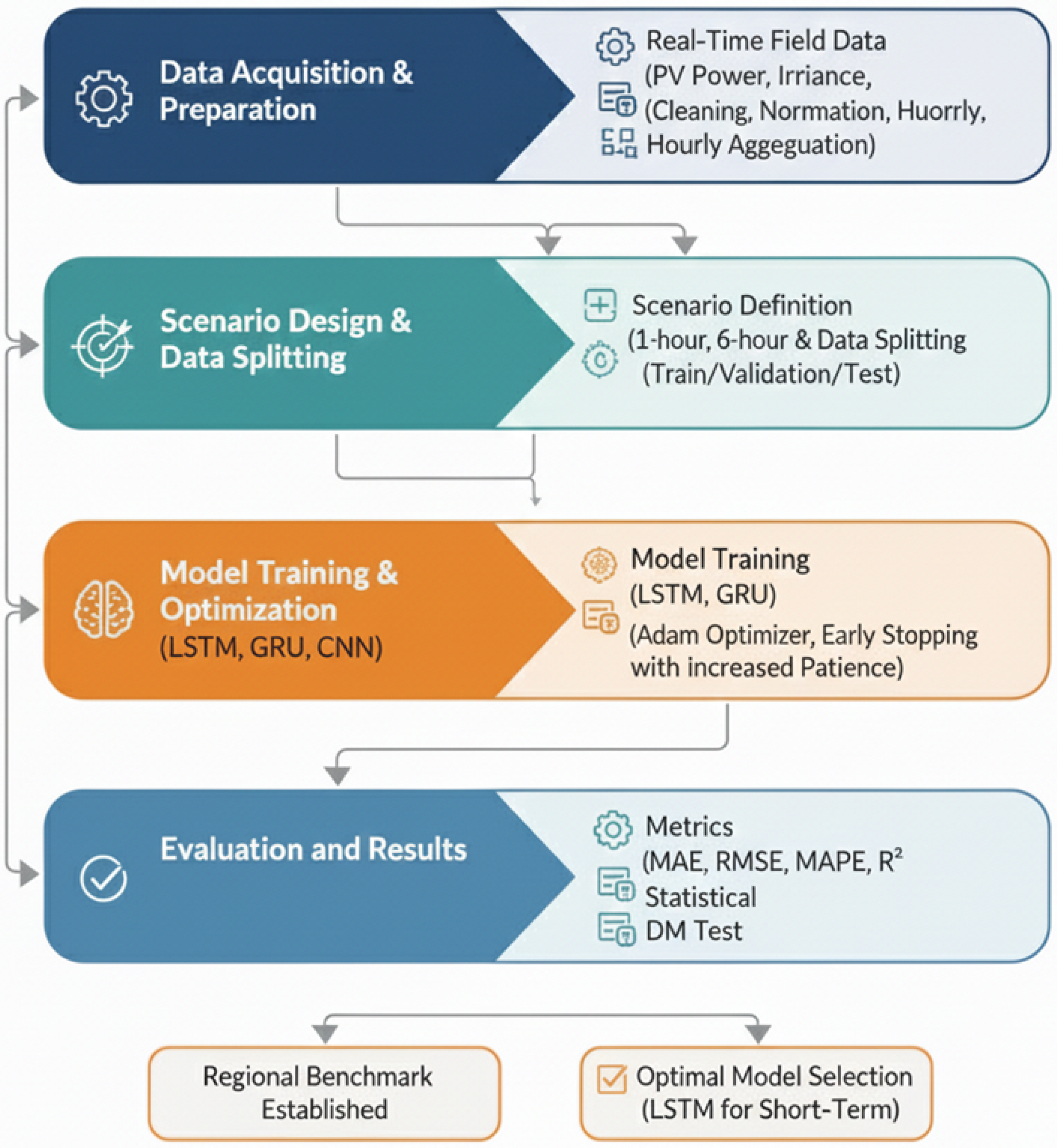
To evaluate the forecasting performance, the dataset was partitioned chronologically to respect the temporal order of the time-series data. The split ratios were set as follows: the first 70% of the data was used for training, the subsequent 15% for validation, and the final 15% for testing. To ensure the reliability of the results and account for the stochastic nature of weight initialization in deep learning models, each experiment was repeated 10 times with different random seeds. The performance metrics reported in this study represent the mean values ± standard deviation of these independent runs. Figure 3 illustrates the overall research workflow adopted in this study, beginning with the acquisition and preparation of real-time field data, including PV power output, irradiance, and environmental variables. Following data cleaning, normalization, and hourly aggregation, multiple forecasting scenarios are constructed by defining different prediction horizons and applying a structured train–validation–test split. The model training stage incorporates LSTM, GRU, and CNN architectures, optimized through the Adam optimizer and an early stopping strategy with increased patience. Finally, model performances are evaluated using MAE, RMSE, MAPE, and metrics, complemented by statistical significance testing. This workflow ensures a rigorous and reproducible framework for experimental setup and data partitioning.
Figure 3.
Research Workflow of the Study.
Table 3 presents the hyperparameter settings used for all models. A unified learning rate of 0.001, Adam optimizer, and a dropout value of 0.2 were applied consistently to ensure fair comparison. LSTM uses a smaller batch size (16) and a deeper hidden structure, whereas CNN and GRU adopt larger batch sizes (64) due to their lighter architectures. Model-specific hidden units reflect the differing complexity levels across LSTM(64→32), CNN(Conv1D 16 filters + Dense 50), and GRU(8 units), ensuring a balanced trade-off between training efficiency and predictive capacity.
Table 3.
Hyperparameter Settings for All Models.
3. Results
This section presents the performance results of the LSTM, CNN, and GRU models developed using actual hourly data obtained from the 250 kWp Dicle University Solar Power Plant (DUSPP). The analysis focuses on short- and medium-term PV power forecasting. The results are comparatively evaluated using error metrics such as the Mean Absolute Error (MAE), Mean Absolute Percentage Error (MAPE), and Root Mean Square Error (RMSE), along with the coefficient of determination (). In addition, the test outcomes provide a comprehensive assessment of model performance under the region’s characteristic climatic and irradiance conditions.
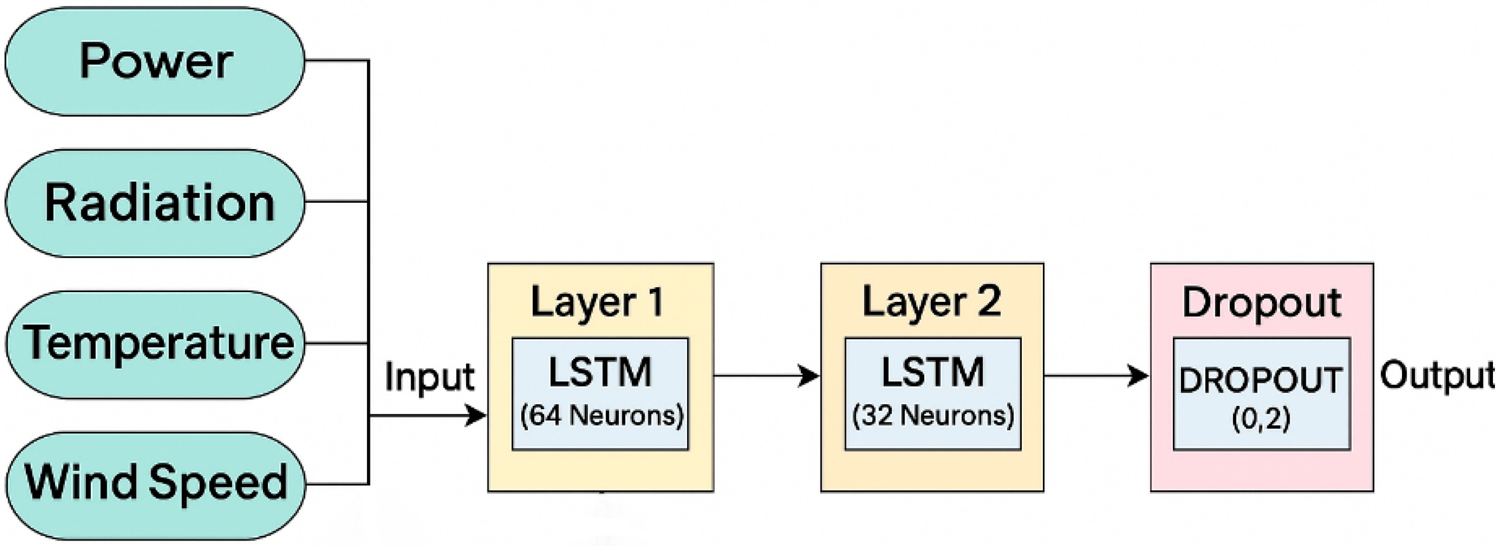
The structure of the LSTM-based model employed in this study is illustrated in Figure 4. The model inputs consist of four principal variables: power, solar radiation, ambient temperature, and wind speed. The first layer includes an LSTM cell with 64 neurons, designed to capture long-term dependencies within the time series data. The second layer is another LSTM layer containing 32 neurons, which further refines and compresses the learned features to enhance representational efficiency. The third and final layer incorporates a dropout rate of 20% (0.2) to prevent overfitting by randomly deactivating a subset of neurons during training. The model output is generated based on the information propagated through these layers. This architecture is specifically optimized for forecasting tasks that depend on time-dependent data, such as solar energy generation.
Figure 4.
Architecture of the LSTM-based model.
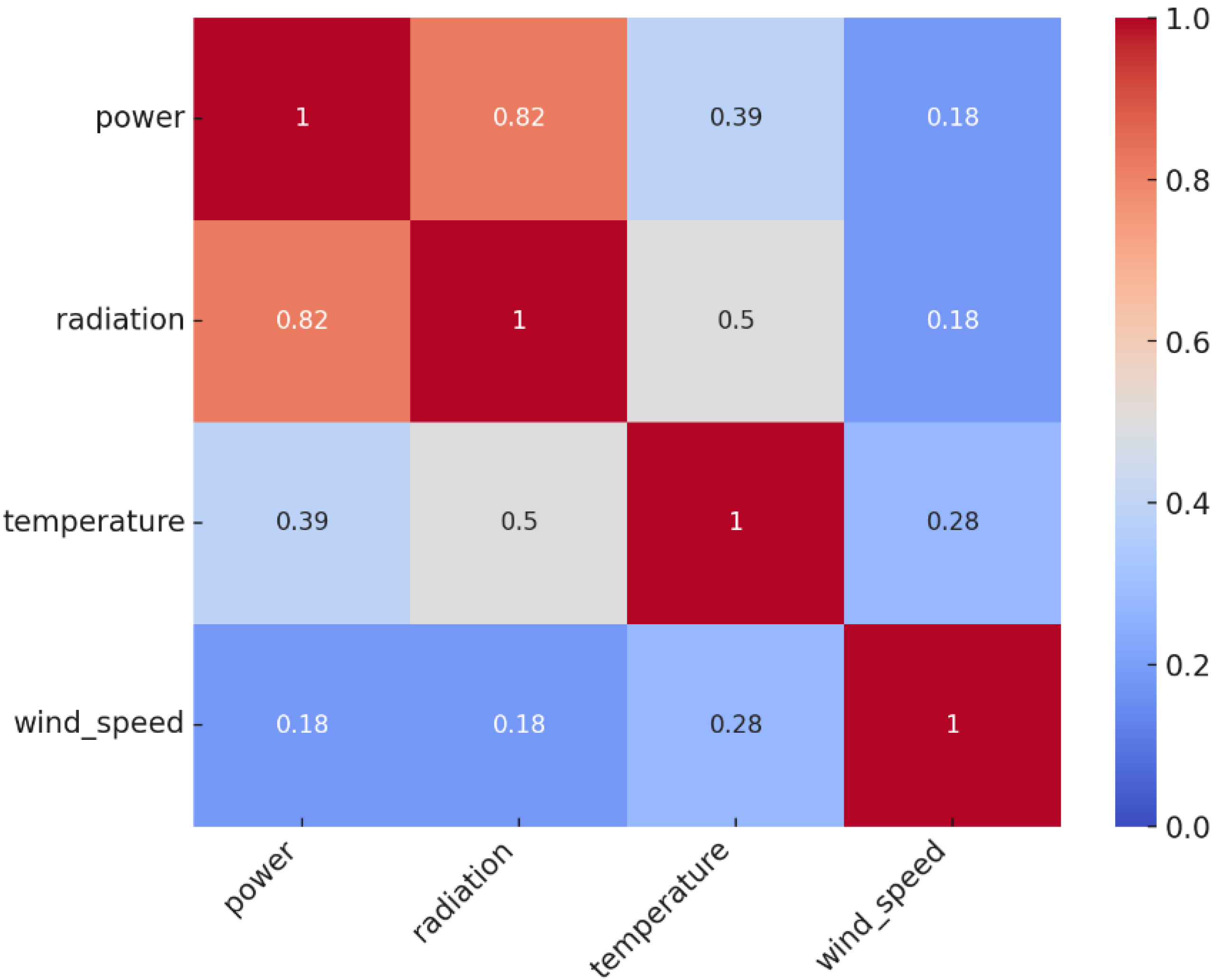
As depicted in Figure 5, the correlation analysis reveals that solar radiation exhibits the strongest positive correlation with PV power output (0.82), confirming its dominant influence on energy generation for the studied region. Ambient temperature demonstrates a moderate correlation with both power output (0.39) and solar radiation (0.50), indicating that thermal conditions have a secondary yet notable effect on PV performance. In contrast, wind speed shows only a weak correlation with the other parameters, implying a negligible role in influencing PV power generation in Southeastern Anatolia. These findings underscore that solar radiation and temperature should be prioritized as key input variables in the proposed deep learning models for short- and medium-term PV power forecasting, whereas wind speed may not significantly enhance prediction accuracy in this specific regional context. Experimental runs without wind speed input yielded negligible differences in error metrics, confirming the correlation analysis results that wind speed contributes minimal predictive power in this specific geographical context compared to irradiance and temperature.
Figure 5.
Correlation matrix of the model input variables.
3.1. Comparative Evaluation of Deep Learning Models
In Table 4, the forecasting scenarios are defined using hourly (H) and daily (D) temporal resolutions. For clarity, an expression such as corresponds to “1-Hour Forecasting Using 6 Hours of Real Data,” meaning that six hours of historical PV power measurements are used as inputs to predict one hour ahead. Similarly, denotes “6-Hour Forecasting Using 12 Hours of Real Data,” while refers to “1-Day Forecasting Using 1 Day of Real Data.” These configurations enable a systematic evaluation of each model under short-term (hourly) and medium-term (daily) forecasting conditions with varying input lengths and prediction horizons.
Table 4.
Test Metrics and Scenarios of Different Deep Learning Models.
Table 4 summarizes the test results of three deep learning architectures—LSTM, CNN, and GRU—across these forecasting scenarios, employing MAE, RMSE, MAPE, and as key performance indicators. An examination of the results shows that the LSTM model consistently outperforms both CNN and GRU across all scenarios. The LSTM achieves the lowest MAE (0.0646 in the 1H→6H scenario), indicating the smallest average deviation from actual PV power values. It also records the lowest RMSE (0.1008), demonstrating enhanced capability in limiting large prediction errors. In terms of MAPE, the LSTM again performs best (19.76%), outperforming the CNN (25.30%) and GRU models (28.58–47.52%), underscoring its robustness across varying temporal resolutions.
The values further reinforce the superiority of the LSTM architecture. Although all models yield moderate values due to the intrinsic variability of solar PV generation, the LSTM achieves the highest coefficient of determination (0.8981), followed by the CNN (0.8422) and GRU (0.7951–0.0300). This indicates that the LSTM explains a larger portion of the variance in PV output and exhibits better generalization capability across forecasting horizons.
Overall, the evidence presented in Table 4 highlights that the LSTM architecture delivers the most accurate and consistent forecasting performance, making it the most suitable deep learning model for short- and medium-term PV power forecasting in the Southeastern Anatolia region.
3.2. Scenario 1: One-Hour Forecasting Using 6 Hours of Real Data
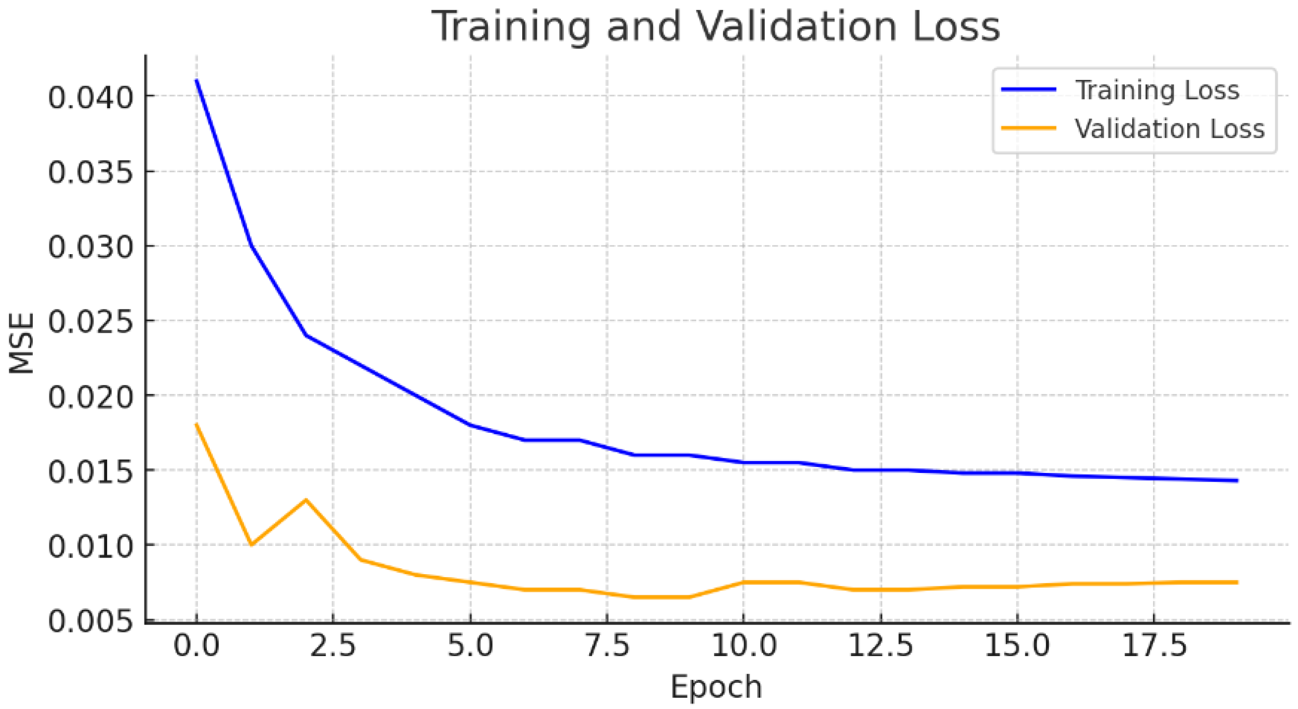
In this scenario, one-hour-ahead forecasting is performed using six hours of historical real PV power data as input. As illustrated in Figure 6, the training loss initially starts at a relatively high value but decreases steadily as the number of epochs increases, indicating that the model successfully adapts to the training data. The validation loss, on the other hand, begins at a lower level compared to the training loss and remains generally stable and low throughout the training process, demonstrating the model’s strong generalization capability. The absence of a significant gap between the training and validation losses suggests a low risk of overfitting.
Figure 6.
Training and validation loss over epochs.
These results indicate that the one-hour-ahead forecasting scenario, based on six hours of real data input, has been successfully optimized, and that the model exhibits stable and reliable performance. In the updated experiments, a higher Early Stopping patience value was employed to prevent premature termination of training. This adjustment allowed the model to continue learning until the validation loss stabilized, resulting in loss curves that reach a clear convergence plateau.
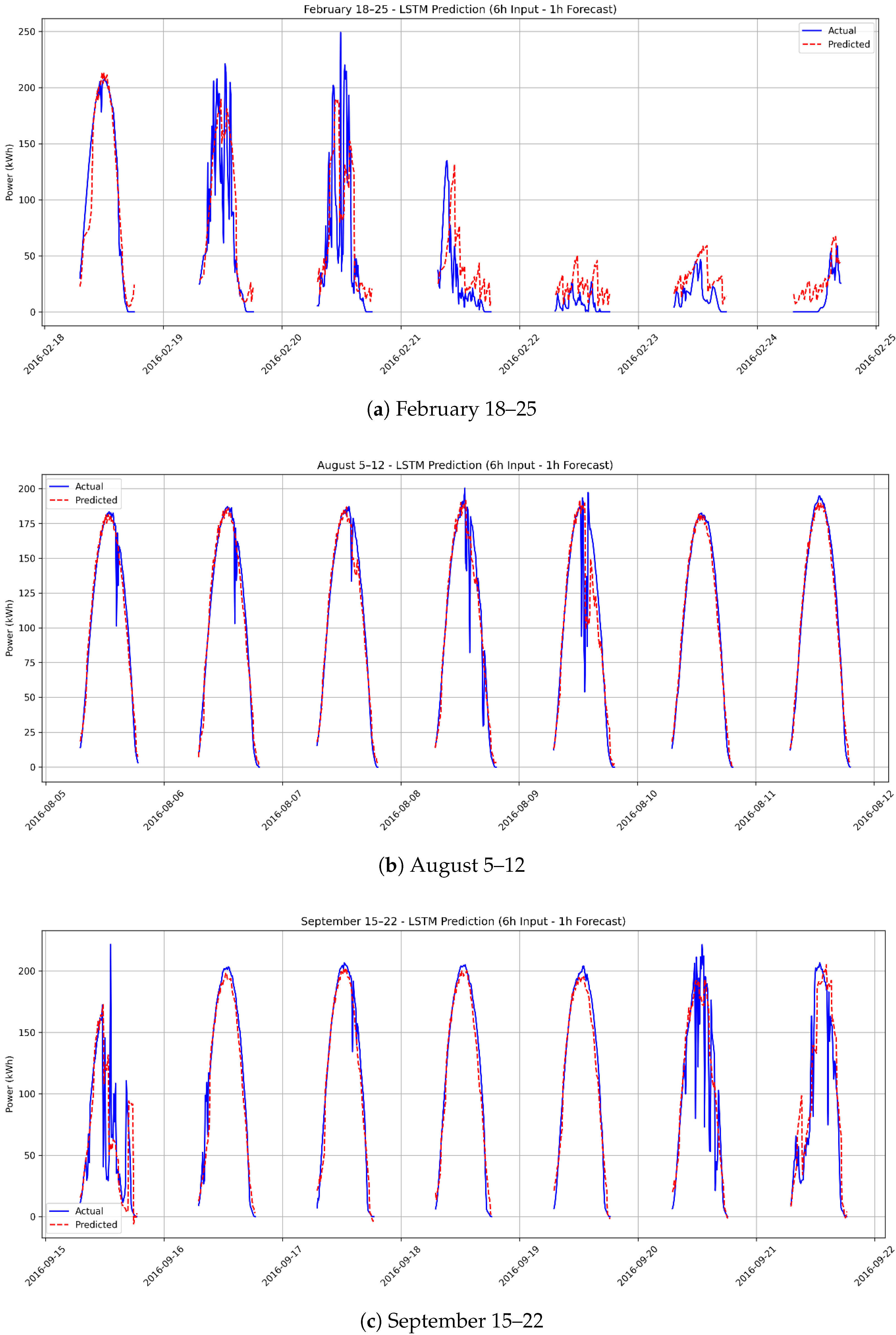
The time-series plots presented in Figure 7 illustrate one-hour-ahead forecasts based on six hours of actual power measurements for the months of February, August, and September. In all three time intervals, the model successfully captures the daily energy production cycles and overall temporal patterns.
Figure 7.
One-hour-ahead PV power forecasts based on six hours of historical data for three different time periods: (a) February 18–25, (b) August 5–12, and (c) September 15–22.
However, during periods characterized by sudden atmospheric changes—such as cloud transients—the forecasting accuracy tends to decline, leading to noticeable deviations from actual power outputs. In contrast, on days with more stable meteorological conditions, the model demonstrates significantly higher predictive accuracy.
Similarly, the time series plot shown in Figure 7b, corresponding to September, further reinforces these findings. While the model retains its ability to learn general patterns effectively, it remains limited in modeling rapid fluctuations induced by abrupt weather variations.
3.3. Scenario 2: Six-Hour Forecasting Using 1 Day of Actual Data
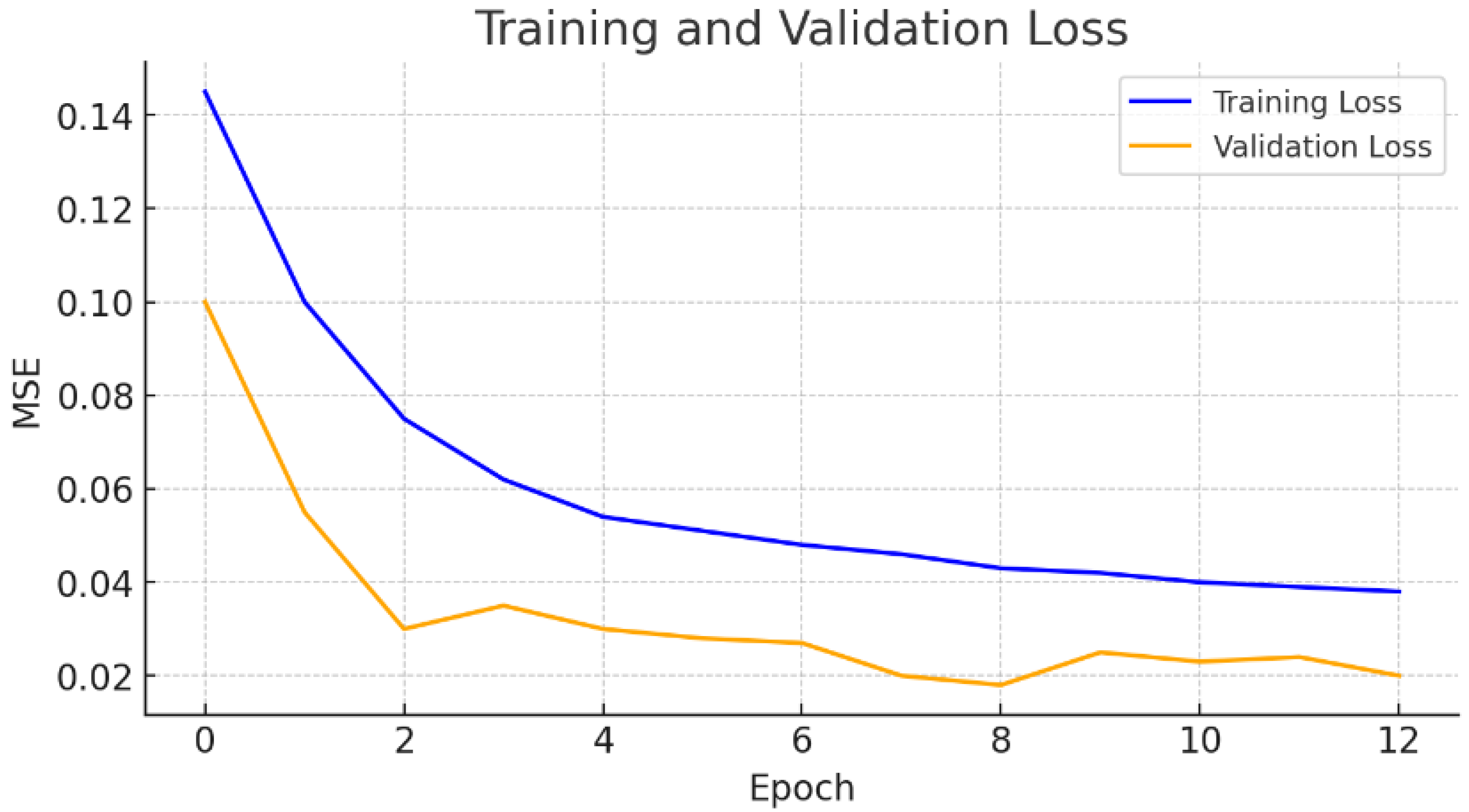
In this scenario, six-hour-ahead forecasting is performed using one full day (24 h) of real PV power data as input. The training and validation loss curves presented in Figure 8 were examined to assess the model’s learning process and generalization capability. The training loss is observed to start at a relatively high value and gradually decrease as the number of epochs increases, indicating successful adaptation to the training data. The validation loss, on the other hand, begins at a value close to the training loss, drops significantly during the early epochs, and then remains stable and low throughout the remaining training process.
Figure 8.
Training and validation loss curves for one-day input data (six-hour-ahead forecast).
The small gap between the training and validation losses suggests a low tendency toward overfitting and highlights the model’s strong generalization ability for unseen data. Furthermore, the plateauing of the validation loss after a certain epoch indicates that the model exhibits stable performance during optimization. These results demonstrate that, in the six-hour-ahead forecasting scenario based on one full day of real data, the model achieves satisfactory prediction accuracy for both the training and validation datasets.
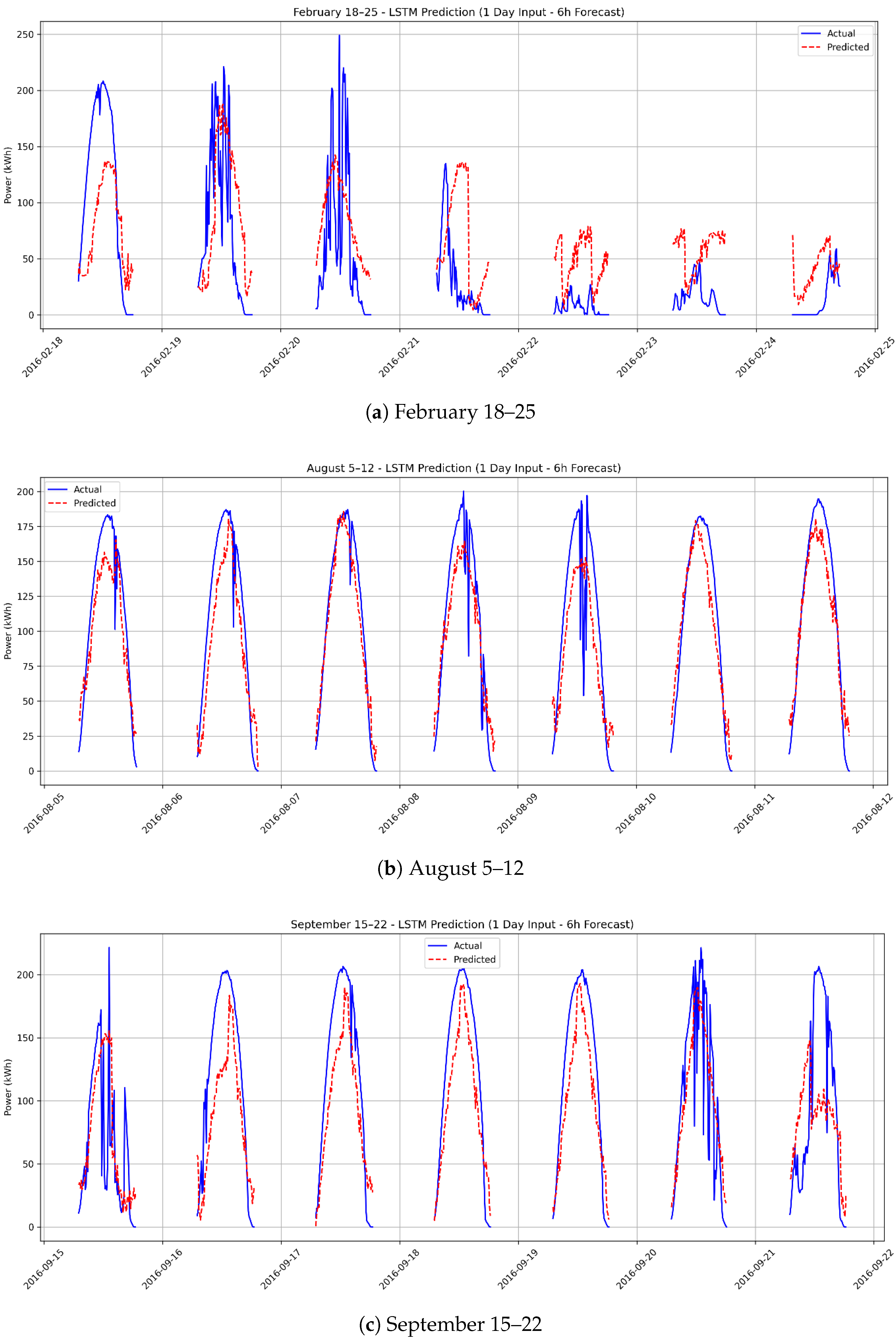
Figure 9b,c, corresponding to August and September, show that even during periods with relatively stable weather conditions, the model exhibits certain limitations in accurately predicting peak power values and abrupt fluctuations. The forecasted peaks often deviate from the actual values, and rapid increases or decreases are not sufficiently captured by the model.
Figure 9.
Six-hour-ahead PV power forecasts based on one-day historical data for three time periods: (a) February 18–25, (b) August 5–12, and (c) September 15–22.
Figure 9a, representing February, reveals a more pronounced decline in forecasting accuracy, primarily due to variable and lower solar irradiance levels. Unpredictable weather variations during this period hindered the model’s ability to generate consistent forecasts based on previous day’s data, resulting in predictions that diverge more significantly from actual measurements.
3.4. Scenario 3: One-Day Forecasting Using 1 Day of Actual Data
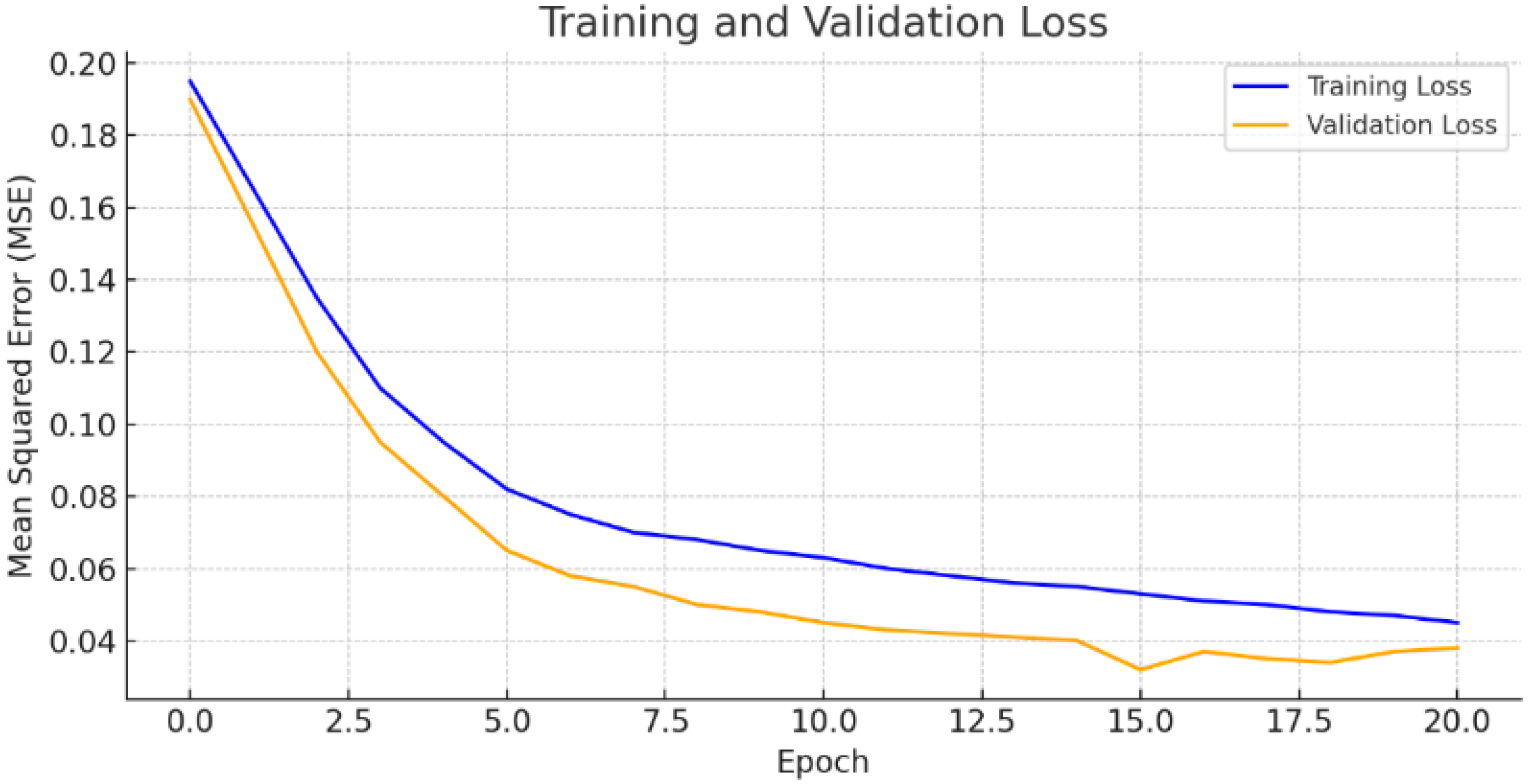
In this scenario, one-day-ahead forecasting is performed using one full day (24 h) of real PV power data as input. Figure 10 illustrates the training and validation loss curves, which assess the model’s learning and generalization performance in the one-day-ahead forecasting scenario using one day of real input data. The training loss initially starts at a relatively high Mean Squared Error (MSE) value (approximately 0.20) and steadily decreases as the number of epochs increases, reaching around 0.045. This indicates that the model successfully fits the training data.
Figure 10.
Training and validation loss curves (one day of real data—one-day-ahead forecast).
Similarly, the validation loss also begins at a high value but drops rapidly, showing a consistent downward trend over the first 20 epochs and closely following the trajectory of the training loss. The fact that the validation loss remains generally lower than the training loss, and that the gap between the two curves does not widen significantly, suggests a low tendency toward overfitting and strong generalization capability to unseen data. These results demonstrate that the model exhibits balanced and consistent performance in the one-day-ahead PV power forecasting scenario using one day of historical input data.
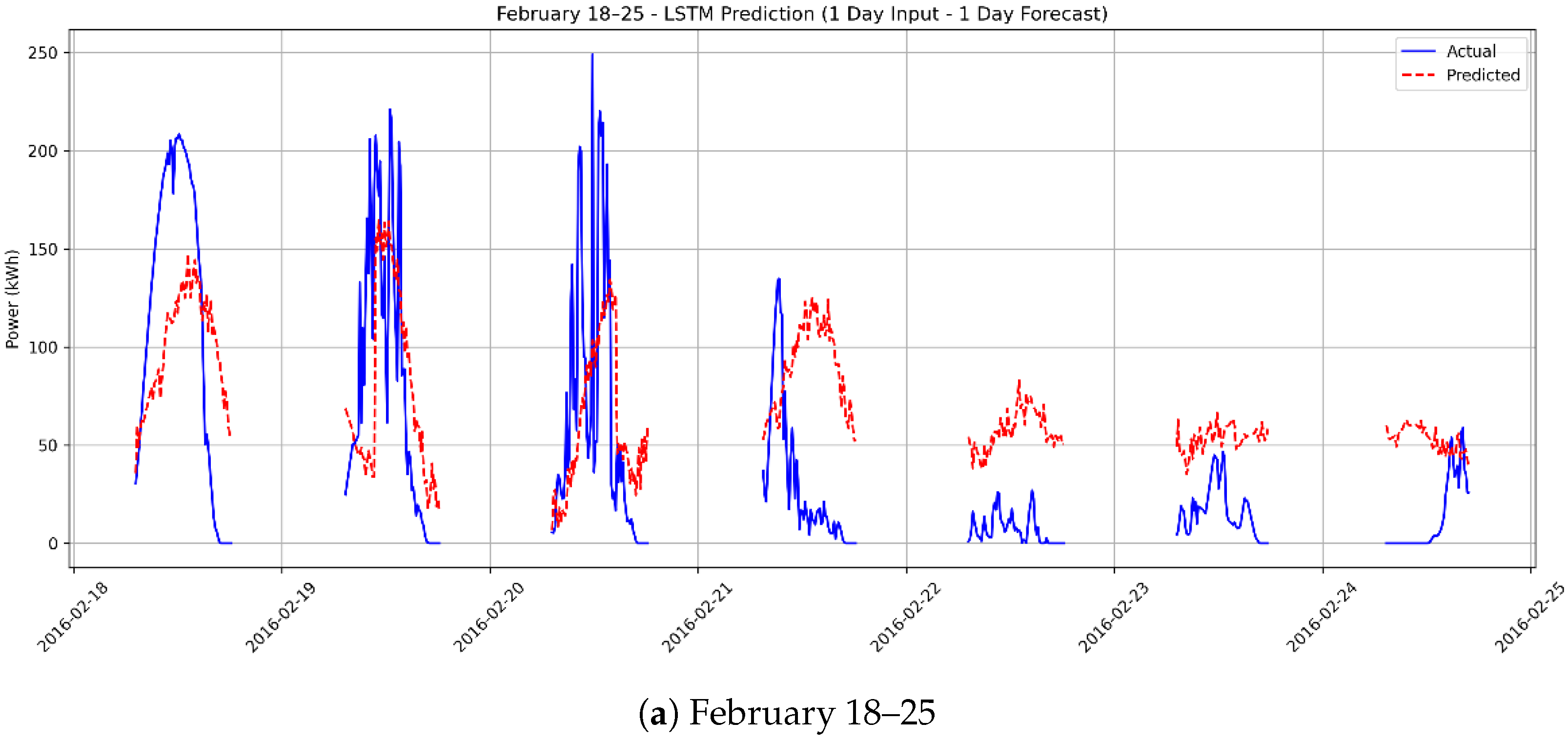
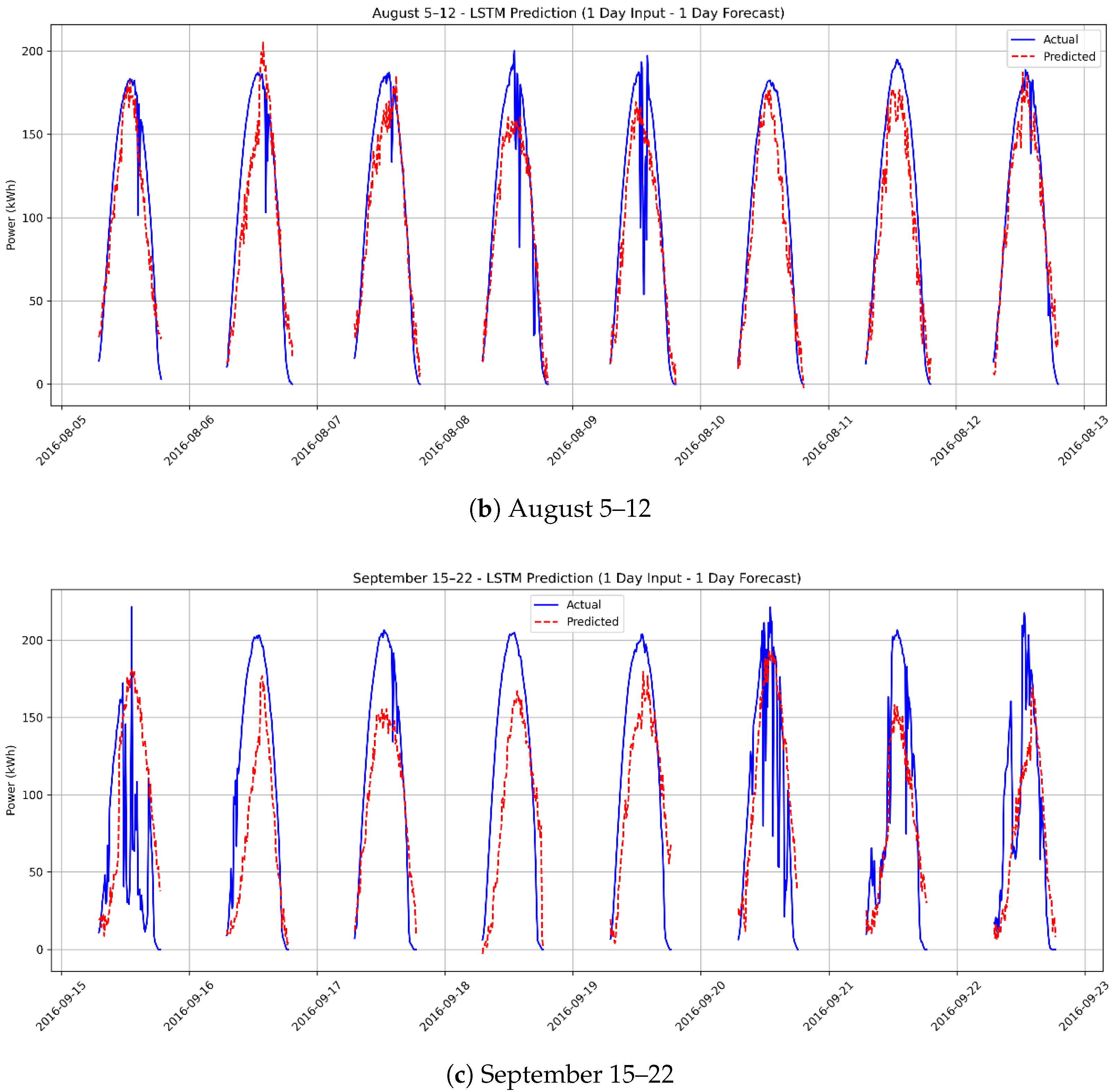
Figure 11 presents a comparative analysis of the forecasting performance of the LSTM deep learning model across different temporal segments—August and September, which generally exhibit stable weather conditions, and February, characterized by more volatile atmospheric patterns. The analysis is conducted over three forecasting horizons: one-hour ahead, six-hour ahead, and one-day ahead.

Figure 11.
One-day-ahead PV power forecasts based on one day of historical data for three different time periods: (a) February 18–25, (b) August 5–12, and (c) September 15–22.
The forecast curves reveal noticeable delays and amplitude mismatches compared to sudden spikes and drops in actual power values. These discrepancies indicate that the model struggles to accurately predict rapid intra-day changes, particularly when relying on data from the previous day. Figure 11b,c, which correspond to August and September, respectively, show that even under relatively stable weather conditions, the model exhibits limitations in accurately capturing peak power values and abrupt fluctuations. Forecasted peak values often deviate from the true peaks, and sudden rises or drops in PV output are not adequately captured by the model.
In contrast, Figure 11a demonstrates an even more pronounced decline in forecasting accuracy. During this period of low and highly variable solar generation, the unpredictability of weather conditions significantly impairs the model’s ability to produce consistent forecasts based on one-day historical input, leading to substantial deviations from actual values.
3.5. Scenario 4: One-Month Ahead Forecasting Using 3 Months of Actual Data
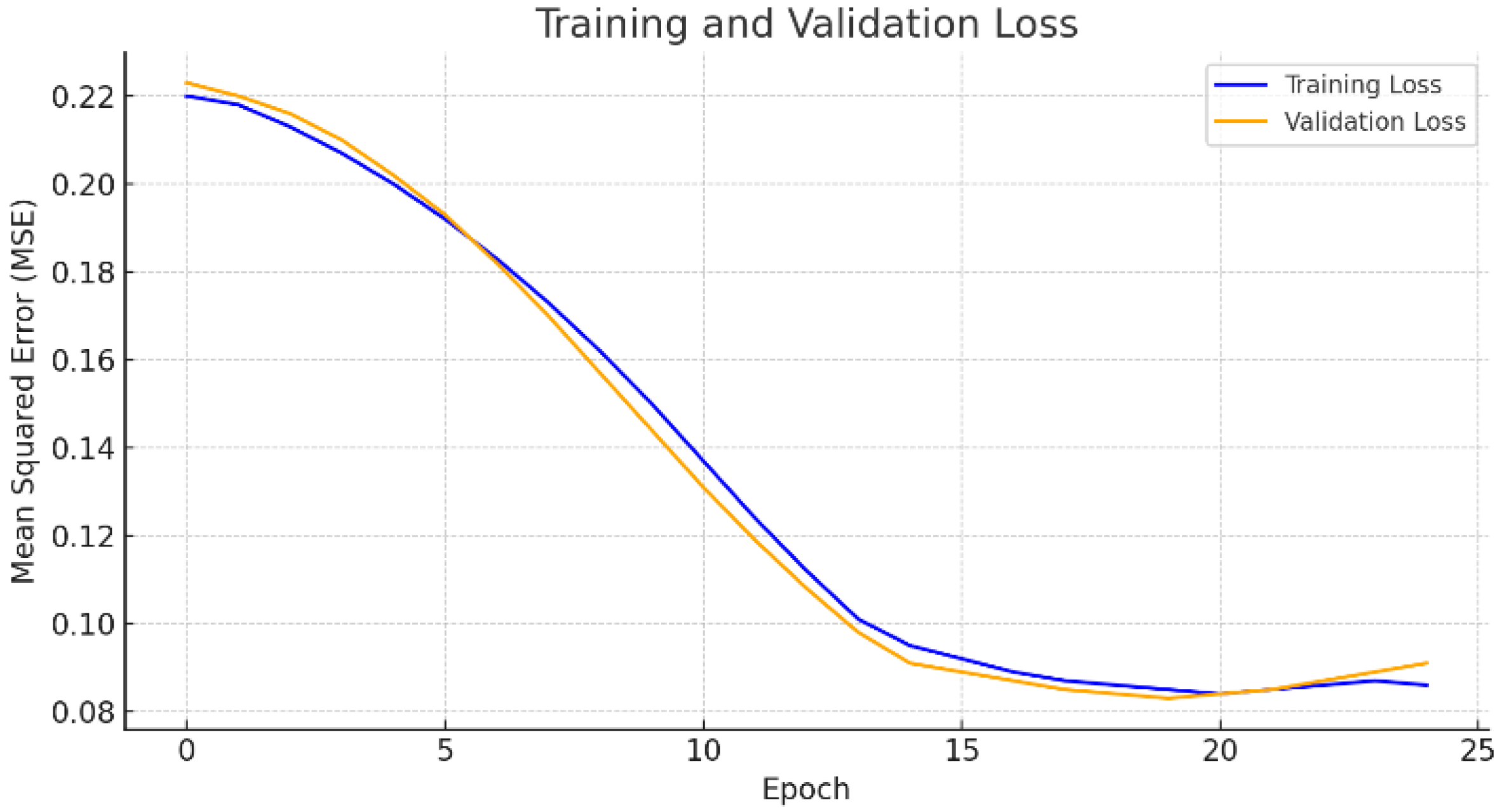
In this scenario, one-month-ahead forecasting is performed using three months of historical PV power data as input. Figure 12 illustrates the training and validation loss curves for the one-month-ahead forecasting scenario based on three months of historical data. As observed in the graph, both the training and validation losses begin with relatively high Mean Squared Error (MSE) values (around 0.22) and steadily decrease as the number of epochs increases. The training and validation loss curves remain closely aligned throughout the training process, indicating that the model maintains a balanced performance—effectively fitting the training data while preserving its generalization ability on unseen validation data.
Figure 12.
Training and validation loss (three months of real data—one-month-ahead forecast).
Notably, in the later epochs, the validation loss remains slightly lower than the training loss, suggesting a low risk of overfitting. This trend demonstrates that the model undergoes a stable optimization process and retains its learning capacity, even in long-term (one-month-ahead) forecasting tasks.
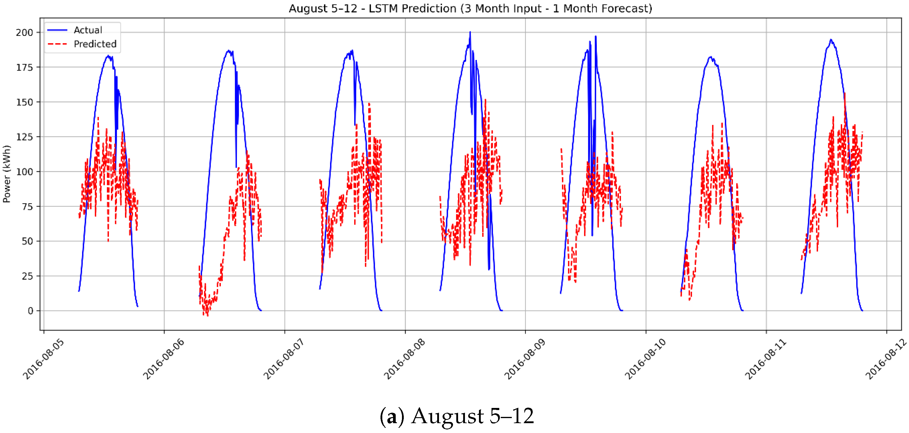
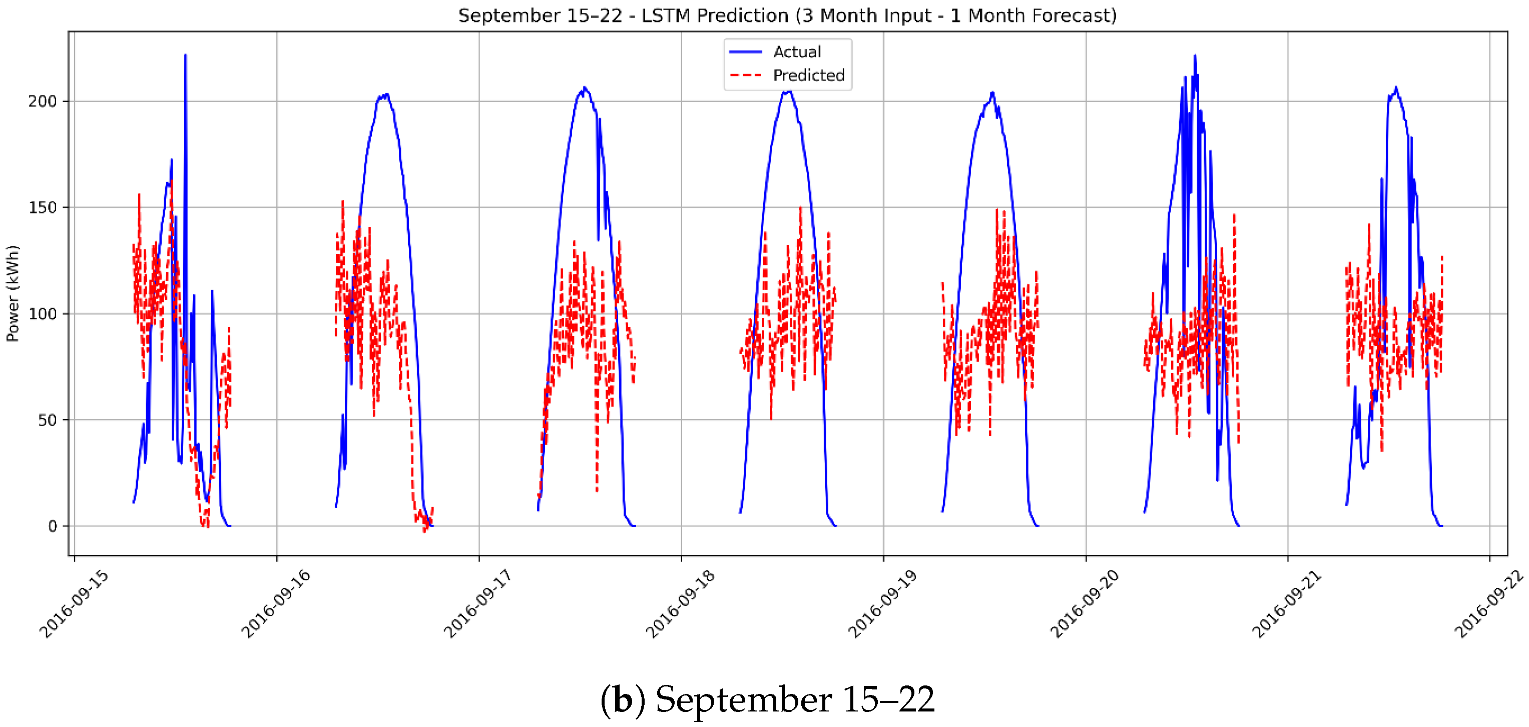
Figure 13a, corresponding to the period August 5–12, demonstrates that the model faces considerable difficulty in tracking actual power values over long-term (one-month-ahead) forecasting horizons. The prediction curve exhibits pronounced high-frequency noise, amplitude mismatches, and phase shifts. These artifacts indicate that the model’s ability to accurately project future trends using past three-month patterns is limited. These observed fluctuations and phase shifts suggest that while the model captures general seasonal trends, its capacity to generalize long-range temporal dependencies diminishes over extended horizons, leading to increased noise during peak irradiance hours. Similarly, Figure 13b, representing the period September 15–22, confirms the model’s low performance in long-term forecasting. The predictions fail to follow the overall shape of the actual power curve, resulting in an irregular and chaotic output. Significant deviations and timing errors are particularly observed at peak and trough points, highlighting the model’s inadequacy in maintaining accuracy over extended forecast horizons.

Figure 13.
One-month-ahead PV power forecasts based on three months of historical data: (a) August 5–12, (b) September 15–22.
4. Conclusions
This study presented a comparative short- and medium-term photovoltaic (PV) power forecasting framework based on real-time meteorological data collected from a 250 kWp grid-connected PV system located at Dicle University, Diyarbakır, Southeastern Anatolia, Turkey. The dataset, which included hourly solar irradiance (average annual GHI 5.4 kWh/m2/day), temperature, humidity, and wind speed, was used to train and validate LSTM, CNN, and GRU models under six forecasting scenarios ranging from 6 h to 1 month.
Limitations and Future Research
Despite the promising results, this study has limitations. First, the dataset spans only one year, which may not fully capture multi-year climatological cycles or extreme outlier events. Second, the performance of all models degraded in the long-term (1-month) forecasting scenario, indicating the need for additional exogenous inputs. Future research will focus on integrating satellite-derived cloud imagery and developing hybrid architectures (e.g., CNN-LSTM) to address these long-horizon inaccuracies. The results demonstrate that the LSTM model consistently provided the best accuracy for short-term forecasts, achieving R2 values above 0.90, with lower MAE and RMSE compared to CNN and GRU models. The GRU model achieved similar performance metrics while requiring approximately 30% less training time, highlighting its efficiency for real-time applications. In contrast, the CNN model produced higher prediction errors due to its limited capacity to capture temporal dependencies in PV generation data. While the standard CNN architecture employed in this comparative baseline struggled with temporal dependencies, it is acknowledged that more complex configurations—such as deeper layers, 1D convolutions specifically tuned for time-series, or hybrid CNN-LSTM architectures—could potentially mitigate these limitations and offer improved performance.
This research confirms that integrating real, site-specific meteorological inputs with advanced deep learning architectures significantly enhances PV power forecasting accuracy, supporting more reliable grid operation and better renewable energy planning. These findings align with previous studies but contribute uniquely by providing a scenario-based multi-model comparison using long-term field data from Southeastern Anatolia, a region with high solar potential.
Future work should explore hybrid deep learning models and real-time adaptive training methods. Additionally, integrating supplementary meteorological features such as cloud cover indices or sky imaging data is planned to further minimize forecast uncertainty, especially under rapidly changing weather conditions. The proposed framework offers a practical tool for regional grid operators, energy managers, and policymakers aiming to increase solar energy penetration while maintaining system stability.
Author Contributions
Conceptualization, E.Y.A., C.H., H.K.; methodology, E.Y.A., C.H., Ö.Y., H.K.; software, K.Ö., Ö.Y., O.K.; validation, C.H., O.K., H.K., Ö.Y.; formal analysis, E.Y.A., K.Ö., C.H., O.K., H.E.; investigation, E.Y.A., K.Ö.; resources, E.Y.A., K.Ö.; data curation, E.Y.A., C.H.; writing—original draft preparation, E.Y.A., K.Ö., C.H.; writing—review and editing, E.Y.A., K.Ö., C.H., O.K., H.K., Ö.Y., H.E.; visualization, E.Y.A., K.Ö., C.H., O.K.; supervision, H.K., Ö.Y.; project administration, H.K., Ö.Y., C.H.; funding acquisition, C.H., H.K., C.H. All authors have read and agreed to the published version of the manuscript.
Funding
This study was supported by the Fırat University Scientific Research Projects Unit (FUBAP) with the project number TEKF.25.53, and the APC was funded by FUBAP.
Institutional Review Board Statement
Not applicable. This study did not involve humans or animals; therefore, ethical approval was not required.
Informed Consent Statement
Not applicable.
Data Availability Statement
The data presented in this study are available on demand from the Cem Haydaroğlu and Heybet Kılıç.
Acknowledgments
This research is supported by the Research Projects Committee of Dicle University (DUBAP) with the project numbers MÜHENDİSLİK.23.008 and MÜHENDİSLİK.23.009. We are grateful to DUBAP for the support.
Conflicts of Interest
Author Hüseyin Erdoğan was employed by Turkish Airlines Inc. at the time of the study. The author declares that this employment did not influence the study design, data analysis, interpretation, or the preparation of the manuscript. The remaining authors declare that the research was conducted in the absence of any commercial or financial relationships that could be construed as a potential conflict of interest.
Abbreviations
The following abbreviations are used in this manuscript:
| IEA | International Energy Agency |
| RES | Renewable Energy Sources |
| PV | Photovoltaic Power |
| EMRA | Energy Market Regulatory Authority |
| RMSE | Root Mean Square Error |
| MAE | Mean Absolute Error |
| MAPE | Mean Absolute Percentage Error |
| LSTM | Long Short Term Memory |
| BiLSTM | Bi-Directional Long Short-Term Memory |
| PCA | Principal Component Analysis |
| DWT | Discrete Wavelet Transform |
| SARIMA | Seasonal Autoregressive Integrated Moving Average |
| CNN | Convolutional Neural Networks |
| GRU | Gated Recurrent Unit |
| NWP | Numerical Weather Prediction |
| AI | Artificial Intelligence |
| DL | Deep Learning |
| GNN | Graph Neural Networks |
References
- International Energy Agency (IEA). World Energy Outlook 2024. 2024. Available online: https://www.iea.org/reports/world-energy-outlook-2024 (accessed on 12 November 2025).
- Demir, E.K.; Haydaroğlu, C.; Kılıç, H.; Çelikpençe, M.; Şahin, M.M. IoT-driven Monitoring and Optimization of Hybrid Energy Storage Systems with Supercapacitors in Distribution Networks. Turk. J. Electr. Power Energy Syst. 2025, 5, 86–95. [Google Scholar] [CrossRef]
- Türk, İ.; Kılıç, H.; Haydaroğlu, C.; Top, A. Robust Load Frequency Control in Hybrid Microgrids Using Type-3 Fuzzy Logic Under Stochastic Variations. Symmetry 2025, 17, 853. [Google Scholar] [CrossRef]
- International Energy Agency (IEA). Electricity Market Report 2023. 2023. Available online: https://www.iea.org/reports/electricity-market-report-2023 (accessed on 12 November 2025).
- Hasnat, M.A.; Asadi, S.; Alemazkoor, N. A graph attention network framework for generalized-horizon multi-plant solar power generation forecasting using heterogeneous data. Renew. Energy 2025, 243, 122520. [Google Scholar] [CrossRef]
- Fan, S.; Geng, H.; Zhang, H. Multi-step power forecasting method for distributed photovoltaic (PV) stations based on multimodal model. Sol. Energy 2025, 298, 113572. [Google Scholar] [CrossRef]
- International Energy Agency (IEA). Renewables 2022: Analysis and Forecast to 2027. 2022. Available online: https://www.iea.org/reports/renewables-2022 (accessed on 12 November 2025).
- Ansong, M.; Huang, G.; Nyang’onda, T.N.; Musembi, R.J.; Richards, B.S. Very short-term solar irradiance forecasting based on open-source low-cost sky imager and hybrid deep-learning techniques. Sol. Energy 2025, 294, 113516. [Google Scholar] [CrossRef]
- Yuan, F.; Chen, Z.; Liang, Y. Precise solar radiation forecasting for sustainable energy integration: A hybrid CEEMD-SCM-GA-LGBM model for day-ahead power and hydrogen production. Renew. Energy 2024, 237, 121732. [Google Scholar] [CrossRef]
- Lo, H.Y.; Wu, Y.K.; Phan, Q.T.; Tan, W.S. A Novel QR-based Probabilistic Forecasting Method for Solar power Generation. IEEE Trans. Ind. Appl. 2025, 61, 5381–5393. [Google Scholar] [CrossRef]
- Mondal, R.; Roy, S.K.; Giri, C. Solar power forecasting using domain knowledge. Energy 2024, 302, 131709. [Google Scholar] [CrossRef]
- Xiong, B.; Chen, Y.; Chen, D.; Fu, J.; Zhang, D. Deep probabilistic solar power forecasting with Transformer and Gaussian process approximation. Appl. Energy 2025, 382, 125294. [Google Scholar] [CrossRef]
- Khan, Z.U.; Khan, A.D.; Khan, K.; Al Khatib, S.A.K.; Khan, S.; Khan, M.Q.; Ullah, A. A review of degradation and reliability analysis of a solar PV module. IEEE Access 2024, 12, 185036–185056. [Google Scholar] [CrossRef]
- Kharazi, S.; Amjady, N.; Nejati, M.; Zareipour, H. A new closed-loop solar power forecasting method with sample selection. IEEE Trans. Sustain. Energy 2023, 15, 687–698. [Google Scholar] [CrossRef]
- Saxena, N.; Kumar, R.; Rao, Y.K.; Mondloe, D.S.; Dhapekar, N.K.; Sharma, A.; Yadav, A.S. Hybrid KNN-SVM machine learning approach for solar power forecasting. Environ. Challenges 2024, 14, 100838. [Google Scholar] [CrossRef]
- Piantadosi, G.; Dutto, S.; Galli, A.; De Vito, S.; Sansone, C.; Di Francia, G. Photovoltaic power forecasting: A Transformer based framework. Energy AI 2024, 18, 100444. [Google Scholar] [CrossRef]
- Lodhi, E.; Dahmani, N.; Bukhari, S.M.S.; Gyawali, S.; Thapa, S.; Qiu, L.; Zafar, M.H.; Akhtar, N. Enhancing microgrid forecasting accuracy with SAQ-MTCLSTM: A self-adjusting quantized multi-task ConvLSTM for optimized solar power and load demand predictions. Energy Convers. Manag. X 2024, 24, 100767. [Google Scholar] [CrossRef]
- Venkateswaran, D.; Cho, Y. Efficient solar power generation forecasting for greenhouses: A hybrid deep learning approach. Alex. Eng. J. 2024, 91, 222–236. [Google Scholar] [CrossRef]
- Erniyazov, S.; Lim, C.G. GNN-enhanced temporal patch segmentation and frequency fusion model for robust solar energy production forecasting. Energy Rep. 2025, 13, 4962–4984. [Google Scholar] [CrossRef]
- Salman, D.; Direkoglu, C.; Kusaf, M.; Fahrioglu, M. Hybrid deep learning models for time series forecasting of solar power. Neural Comput. Appl. 2024, 36, 9095–9112. [Google Scholar] [CrossRef]
- Panamtash, H.; Mahdavi, S.; Sun, Q.Z.; Qi, G.J.; Liu, H.; Dimitrovski, A. Very short-term solar power forecasting using a frequency incorporated deep learning model. IEEE Open Access J. Power Energy 2023, 10, 517–527. [Google Scholar] [CrossRef]
- Liu, M.; Ling, Q. Spatial–temporal multimodal fusion model for intra-hour solar power forecasting under variable weather conditions. Renew. Energy 2025, 248, 123043. [Google Scholar] [CrossRef]
- Kim, J.; Obregon, J.; Park, H.; Jung, J.Y. Multi-step photovoltaic power forecasting using transformer and recurrent neural networks. Renew. Sustain. Energy Rev. 2024, 200, 114479. [Google Scholar] [CrossRef]
- Aksoy, N.; Yilmaz, A.; Bayrak, G.; Koç, M. Eliminating Meteorological Dependencies in Solar Power Forecasting: A Deep Learning Solution with NeuralProphet and Real-World Data. IEEE Access 2025, 13, 93287–93301. [Google Scholar] [CrossRef]
- Visser, L.; AlSkaif, T.; Hu, J.; Louwen, A.; van Sark, W. On the value of expert knowledge in estimation and forecasting of solar photovoltaic power generation. Sol. Energy 2023, 251, 86–105. [Google Scholar] [CrossRef]
- Sun, Y.; Venugopal, V.; Brandt, A.R. Short-term solar power forecast with deep learning: Exploring optimal input and output configuration. Sol. Energy 2019, 188, 730–741. [Google Scholar] [CrossRef]
- Wang, J.; Zhang, Z.; Xu, W.; Li, Y.; Niu, G. Short-Term Photovoltaic Power Forecasting Using a Bi-LSTM Neural Network Optimized by Hybrid Algorithms. Sustainability 2025, 17, 5277. [Google Scholar] [CrossRef]
- Suanpang, P.; Jamjuntr, P. Machine learning models for solar power generation forecasting in microgrid application implications for smart cities. Sustainability 2024, 16, 6087. [Google Scholar] [CrossRef]
- Perera, M.; De Hoog, J.; Bandara, K.; Senanayake, D.; Halgamuge, S. Day-ahead regional solar power forecasting with hierarchical temporal convolutional neural networks using historical power generation and weather data. Appl. Energy 2024, 361, 122971. [Google Scholar] [CrossRef]
- Song, Z.; Xiao, F.; Chen, Z.; Madsen, H. Probabilistic ultra-short-term solar photovoltaic power forecasting using natural gradient boosting with attention-enhanced neural networks. Energy AI 2025, 20, 100496. [Google Scholar] [CrossRef]
- Hu, B.; Shao, H.; Shao, C.; Tang, W. A satellite-based novel method to forecast short-term (10 min–4 h) solar radiation by combining satellite-based cloud transmittance forecast and physical clear-sky radiation model. Sol. Energy 2025, 290, 113376. [Google Scholar] [CrossRef]
- Mauladdawilah, H.; Balfaqih, M.; Balfagih, Z.; Pegalajar, M.d.C.; Gago, E.J. Deep Feature Selection of Meteorological Variables for LSTM-Based PV Power Forecasting in High-Dimensional Time-Series Data. Algorithms 2025, 18, 496. [Google Scholar] [CrossRef]
- Di Leo, P.; Ciocia, A.; Malgaroli, G.; Spertino, F. Advancements and Challenges in Photovoltaic Power Forecasting: A Comprehensive Review. Energies 2025, 18, 2108. [Google Scholar] [CrossRef]
- Palm, S.F.; Gomna, A.; Kadri, S.M.; Bonkoungou, D.; Ouedraogo, A.L.; Soro, Y.M.; Sawadogo, M. Performance Study and Implementation of Accurate Solar PV Power Prediction Methods for the Nagréongo Power Plant in Burkina Faso. Energies 2025, 18, 5285. [Google Scholar] [CrossRef]
- Cican, G.; Buturache, A.N.; Silivestru, V. Predicting Photovoltaic Energy Production Using Neural Networks: Renewable Integration in Romania. Processes 2025, 13, 2219. [Google Scholar] [CrossRef]
- Song, N.; Chang-Silva, R.; Lee, K.; Park, S. Dynamic Model Selection in a Hybrid Ensemble Framework for Robust Photovoltaic Power Forecasting. Sensors 2025, 25, 4489. [Google Scholar] [CrossRef]
- Joo, Y.; Kim, D.; Noh, Y.; Choi, J.; Lee, J. Performance Comparison of LSTM and ESN Models in Time-Series Prediction of Solar Power Generation. Sustainability 2025, 17, 8538. [Google Scholar] [CrossRef]
- Massidda, L.; Bettio, F.; Marrocu, M. Probabilistic day-ahead prediction of PV generation. A comparative analysis of forecasting methodologies and of the factors influencing accuracy. Sol. Energy 2024, 271, 112422. [Google Scholar] [CrossRef]
- Haydaroğlu, C.; Kılıç, H.; Gümüş, B. Performance Analysis and Comparison of Performance Ratio of Solar Power Plant. Turk. J. Electr. Power Energy Syst. 2024, 4, 190–199. [Google Scholar] [CrossRef]
- Gumus, B.; Kilic, H. Time dependent prediction of monthly global solar radiation and sunshine duration using exponentially weighted moving average in southeastern of Turkey. Therm. Sci. 2018, 22, 943–951. [Google Scholar] [CrossRef]
- Huang, W.; Zhang, W.; Chen, Q.; Feng, B.; Li, X. Prediction algorithm for power outage areas of affected customers based on CNN-LSTM. IEEE Access 2024, 12, 15007–15015. [Google Scholar] [CrossRef]
- Özdemir, Ş.; Demir, Y.; Yildirim, Ö. The effect of input length on prediction accuracy in short-term multi-step electricity load forecasting: A CNN-LSTM approach. IEEE Access 2025, 13, 28419–28432. [Google Scholar] [CrossRef]
- Yildirim, Ö. A novel wavelet sequence based on deep bidirectional LSTM network model for ECG signal classification. Comput. Biol. Med. 2018, 96, 189–202. [Google Scholar] [CrossRef]
- Yildirim, O.; Baloglu, U.B.; Tan, R.S.; Ciaccio, E.J.; Acharya, U.R. A new approach for arrhythmia classification using deep coded features and LSTM networks. Comput. Methods Programs Biomed. 2019, 176, 121–133. [Google Scholar] [CrossRef] [PubMed]
- Wang, L.; Liu, Y.; Li, T.; Xie, X.; Chang, C. Short-term PV power prediction based on optimized VMD and LSTM. IEEE Access 2020, 8, 165849–165862. [Google Scholar] [CrossRef]
- Yu, C.; Qi, X.; Ma, H.; He, X.; Wang, C.; Zhao, Y. LLR: Learning learning rates by LSTM for training neural networks. Neurocomputing 2020, 394, 41–50. [Google Scholar] [CrossRef]
- Geng, D.; Zhang, H.; Wu, H. Short-term wind speed prediction based on principal component analysis and LSTM. Appl. Sci. 2020, 10, 4416. [Google Scholar] [CrossRef]
- Gers, F.A.; Schmidhuber, J.; Cummins, F. Learning to forget: Continual prediction with LSTM. Neural Comput. 2000, 12, 2451–2471. [Google Scholar] [CrossRef]
Disclaimer/Publisher’s Note: The statements, opinions and data contained in all publications are solely those of the individual author(s) and contributor(s) and not of MDPI and/or the editor(s). MDPI and/or the editor(s) disclaim responsibility for any injury to people or property resulting from any ideas, methods, instructions or products referred to in the content. |
© 2025 by the authors. Licensee MDPI, Basel, Switzerland. This article is an open access article distributed under the terms and conditions of the Creative Commons Attribution (CC BY) license (https://creativecommons.org/licenses/by/4.0/).