CFD Investigation of Free-Surface-Pressurized Flow and Air-Vent Optimization in Combined Tailrace–Diversion Systems

Abstract

This study investigates the hydraulic transient behavior and optimization of air-vent configurations in the combined tailrace–diversion system of a hydropower station. The inlet flow boundary conditions were derived from the method of characteristics (MOC), and flow variations were incorporated into the CFD model using a user-defined function (UDF). The CFD results were validated by comparing them to MOC-based simulations of surge oscillations in the downstream chamber. Six different air-vent configurations, varying in number and diameter, were tested under high-water-level load-acceptance and load-rejection conditions. The results demonstrate that increasing the vent diameter, particularly to 3 m, significantly improves pressure regulation and air exchange efficiency, enhancing system stability. In contrast, simply increasing the number of vents did not lead to noticeable improvements. Sensitivity analysis of vent height revealed that raising the vent height from 12 m to 15 m provides sufficient freeboard to prevent overflow, without overdesign. These findings provide practical guidance for optimizing air-vent configurations in hydropower tailrace systems, improving hydraulic stability, and ensuring safe operation.

1. Introduction

The global energy structure is undergoing a transformation driven by carbon neutrality goals, resulting in rapid advancements in renewable energy sources such as wind and solar power [1]. However, the intermittency and volatility of these resources present significant challenges to the stability and reliability of power systems. Hydropower, characterized by its low-carbon, renewable, and highly flexible nature [2,3,4], continues to play a vital role in meeting global energy demands and remains a cornerstone of the clean energy transition [5,6]. As the demand for stable and reliable renewable generation increases, the hydraulic stability of hydropower stations during transient processes, especially under complex hydrological and extreme climatic conditions, has become a critical area of focus [7,8,9].

Among various hydropower plant layouts, the combined tailrace–diversion configuration has gained widespread adoption due to its terrain adaptability and cost-effectiveness. This “one-tunnel-for-multiple-uses” approach repurposes a diversion tunnel as part of the power tailrace, effectively shortening the waterway, reducing construction costs, and enabling more compact plant arrangements [10]. In many large diversion hydropower projects, a fully constructed diversion tunnel can later be converted into a tailrace, further reducing construction timelines and accelerating project delivery [11]. This design concept has also been widely adopted in hydropower projects, where diversion tunnels are integrated into tailrace systems to enhance hydraulic behavior and overall operating efficiency [12].

However, due to the typically higher invert elevation of the diversion tunnel compared to the tailrace, the conversion results in frequent alternations between pressurized and free-surface flow states (mixed flow), which causes significant pressure pulsations. These pulsations can lead to lining damage and pose serious risks to operational safety. During hydraulic transients, rapid pressure changes and surge motions can easily generate low-pressure zones at higher elevations. Once the local pressure drops to the vapor-pressure level, vapor pockets or cavitation may occur, potentially leading to column separation. These vapor-related phenomena are distinct from water-hammer pressure waves, although both may arise during rapid transient processes and pose risks to operational safety [13,14]. To mitigate these adverse transients and improve stability, air-vent systems are commonly employed.

Research on mixed free-surface-pressurized flow in hydropower tailrace tunnels, together with venting measures, has advanced significantly in recent years. Zhou [15] investigated the transition characteristics between free-surface and pressurized flow in ceiling-sloping tail tunnels, emphasizing that accurate modeling of the moving interface is critical for evaluating hydraulic stability. Guo [16] examined unsteady flow behavior in large-scale tailrace tunnels and revealed that periodic jetting and flow alternation phenomena are strongly influenced by downstream water-level variations, which can amplify transient pressure fluctuations. Subsequently, researchers have proposed a variety of numerical approaches to improve the predictive accuracy of mixed-flow transients. The implicit characteristic method has been widely applied to simulate the alternation between free-surface and pressurized flow [17], providing a solid foundation for subsequent three-dimensional CFD simulations. Building upon this foundation, further investigations using the volume of fluid (VOF) model have quantitatively analyzed the influence of air-vent geometry on system stability, enabling high-resolution visualization of air–water interface evolution and transient pressure variations [18,19]. Comparative analyses have shown that 1D–3D coupling methods outperform traditional virtual-slot models in predicting complex mixed-flow dynamics [20]. Recent CFD investigations of air–water two-phase flow in hydraulic tunnel systems have shown that air entrainment and water–air interaction significantly influence transient pressure evolution and flow stability during mixed flow conditions [21]. From a numerical perspective, combining implicit characteristic schemes with Newton–Raphson linearization enhances the accuracy of free-surface pressurized flow modeling [22], and parametric analyses further indicate that increasing vent diameter within an optimal range can effectively reduce maximum tunnel pressure [23]. Collectively, these studies provide a robust theoretical and computational foundation for the design and optimization of venting systems in mixed-flow tailrace tunnels.

Despite significant advancements, critical gaps remain in understanding the transient behavior of vented mixed flows. Venting induces localized two-phase dynamics within the tunnel, where rapid air expansion and compression cycles can lead to intense short-duration pressure spikes and water ejection at the outlet, particularly when the design is suboptimal. Existing studies provide limited quantitative insights into these rapid transients, and the phenomenon of transient over-pressurization at vents has not been fully recognized. Recent work has made strides by linearizing 1D two-phase transient equations, validated against classical single-phase benchmarks [24], and exploring air–water interaction mechanisms in combined diversion-tailrace systems through experiments [25]. Additionally, 1D–3D coupling methods have been used to analyze transient air–water patterns in vent tubes, providing valuable foundational insights into the mechanisms involved [26]. However, a systematic evaluation that connects vent geometry—such as number, diameter, and height—to measurable transient risks, including negative-pressure mitigation, peak intake/exhaust velocity, and overflow potential, under realistic operating scenarios, is still lacking.

In this study, a CFD computational framework driven by MOC-based boundary conditions is developed to analyze the hydraulic transient behavior of a combined tailrace–diversion system and optimize air-vent configuration. The VOF model, coupled with the SST turbulence model, is employed to capture transient air–water interface dynamics during load-acceptance and load-rejection processes. The research focuses on (i) establishing a reliable modeling framework that integrates 1D transient results into 3D simulations, (ii) investigating the influence of vent number and diameter on pressure regulation and air exchange, and (iii) conducting a sensitivity study of vent height to provide design guidance for preventing transient overflow. This study aims to provide a physically grounded reference for the safe and efficient design of air-vent systems in large-scale hydropower tailrace tunnels.

The remainder of the paper is organized as follows: Section 2 presents the methodology, including the virtual-slot formulation, the VOF multiphase model, the 3D geometry/mesh, and the boundary-condition strategy that incorporates 1D characteristic results into the 3D inlet. Section 3 reports model validation and analyzes surge oscillations, followed by sensitivity studies on vent number/diameter and vent height under representative high-water-level transients. Section 4 provides a detailed discussion of the results, highlighting the implications for air-vent configuration optimization and hydraulic transient behavior. Section 5 concludes the paper with the key findings.

2. Methodology

2.1. Virtual Slot Method

For combined draft and tailrace systems, the flow alternates between pressurized and free-surface states, forming a mixed flow regime. To accurately describe this behavior, the governing equations of unsteady pressurized flow and unsteady open-channel flow must be coupled, with proper treatment of the interface transition.

The unsteady pressurized flow equations are as follows:

$${\displaystyle \frac{\partial V}{\partial t}}+V{\displaystyle \frac{\partial V}{\partial x}}+g{\displaystyle \frac{\partial H}{\partial x}}+{\displaystyle \frac{f}{2D}}V\left|V\right|=0$$

(1)

$${\displaystyle \frac{\partial H}{\partial t}}+V{\displaystyle \frac{\partial H}{\partial x}}-V\sin \alpha +{\displaystyle \frac{a^2}{g}}{\displaystyle \frac{\partial V}{\partial x}}=0$$

(2)

where

V is the flow velocity in the conduit (positive from upstream to downstream);

H is the piezometric head;

t is time;

x is the longitudinal coordinate along the tunnel;

g is the gravitational acceleration;

f is the Darcy–Weisbach friction factor;

D is pipe diameter;

α is the inclination angle of the conduit axis;

a is the wave speed of the water hammer.

The Saint–Venant equations for open-channel flow are as follows:

$$B{\displaystyle \frac{\partial H}{\partial t}}+{\displaystyle \frac{\partial Q}{\partial x}}=0$$

(3)

$${\displaystyle \frac{\partial Q}{\partial t}}+{\displaystyle \frac{\partial }{\partial x}}\left({\displaystyle \frac{Q^2}{A}}\right)+gA{\displaystyle \frac{\partial H}{\partial x}}+g{\displaystyle \frac{Q\left|Q\right|}{A{C}^{2}R}}=0$$

(4)

where

B is the width of the free surface;

Q is the discharge;

h is the water surface head;

A is the flow area;

D is the diameter of the tunnel section;

S_f is the friction slope;

C is the Chézy coefficient;

R is the hydraulic radius.

Equations (1) and (2) correspond to the one-dimensional continuity and momentum equations for pressurized pipe flow, derived using the method of characteristics (MOC). Equations (3) and (4) are the Saint–Venant equations for unsteady open-channel flow. These formulations are widely used in transient hydraulic analysis and provide a well-established theoretical basis for modelling mixed pressurized and free-surface flow conditions in diversion tunnels [27].

The virtual slot method assumes a narrow fictitious slit at the top of the conduit that does not change its flow area, thereby transforming pressurized flow into an equivalent open-channel flow [27]. The slot width B is defined such that the gravity wave speed equals the pressure wave speed c:

$$c=\sqrt{gA/B}=a$$

(5)

This approach allows for unified simulation of mixed pressurized and free-surface flow within a single set of equations, simplifying numerical implementation while maintaining physical consistency.

2.2. VOF Multiphase Flow Model

The VOF model is employed to simulate transient air–water interactions in the tailrace system of a hydropower station, particularly during load transitions. It effectively captures complex two-phase flow phenomena, such as pressure fluctuations and cavitation risks, by modeling gas–liquid interfaces within the tailrace tunnel. By tracking the volume fractions of each phase, the model provides critical insights for optimizing air-vent configurations and ensuring the stable operation of the tailrace system [28].

The VOF model assumes immiscibility between phases. Each phase’s volume fraction is defined within the control volume, with the sum of all phase fractions equaling 1. The properties and variables of the flow field are shared by all phases and represented as volume-averaged quantities. The interface between phases is tracked using the continuity equation for the volume fraction of each phase, as shown in the following form:

$${\displaystyle \frac{1}{{\rho }_q}}\left[{\displaystyle \frac{\partial }{\partial t}}\left({\alpha }_q{\rho }_q\right)+\nabla \cdot \left({\alpha }_q{\rho }_q{u}_q\right)\right]=S_{{\alpha }_q}+{\displaystyle \sum _{p=1}^n\left({\dot{m}}_{pq}-{\dot{m}}_{qp}\right)}$$

(6)

where ${\alpha }_q$ is the volume fraction of phase q; ${\dot{m}}_{pq}$ and ${\dot{m}}_{qp}$ represent the mass transfer between phases q and p.

For the initial phase, the volume fraction equation is not solved directly but is determined based on the constraint that the sum of the volume fractions of all phases must equal 1:

$${\displaystyle \sum _{q=1}^n{\alpha }_q}=1$$

(7)

2.3. 3D Model and Mesh Generation

During the transient process, the mixed-flow phenomenon primarily occurs at the junction between the tailrace pipe and the diversion tunnel. The focus of the simulation is to investigate the air–water interaction and pressure fluctuations, and their impact on the hydraulic structures along the tunnel. Consequently, the computational model encompasses the entire pipeline, from beneath the turbine runner to the tailrace outlet, including the downstream surge chamber and the large diversion tunnel. The tailrace pipe has a circular cross-section with an internal diameter of approximately 14.50 m and extends about 327.37 m before joining the diversion tunnel. The diversion tunnel adopts a rectangular section with a circular-arch roof, formed by vertical sidewalls and an arch with a radius of 7.79 m. The invert width is about 13 m, and the vertical sidewalls are approximately 13.5 m in height. From the junction, the tunnel extends 1055.73 m downstream to the tailrace outlet. In the baseline air-vent configuration (Type 1), four vertical ventilation shafts are arranged along the tunnel crown. Each shaft has a diameter of 2.0 m and a height of about 12 m, with an axial spacing of approximately 51.20 m between adjacent vents. The tailrace pipe outlet is located at an elevation of 2718.16 m, the surge chamber floor is at 2735 m, the diversion tunnel floor is at 2752 m, and the tailrace tunnel outlet is at 2751 m. The overall model, along with the detailed modeling of the four main hydraulic structures, is shown in Figure 1, which also includes the pressure monitoring point (up1) located at the top of the tailrace–diversion junction.

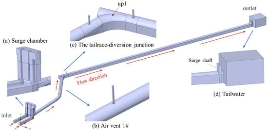
Figure 1. The 3D model of the tailrace system.

The computational mesh was generated using a hybrid hexahedral–polyhedral topology to balance numerical accuracy and computational efficiency. Local mesh refinement was applied to key areas, including around the air vents, the junction between the tailrace and diversion tunnels, and the downstream outlet region, to capture detailed flow variations. The mesh details are shown in Figure 2. Mesh convergence was preliminarily assessed by comparing surge wave variations in the surge chamber for different grid densities. The final mesh consists of approximately 3.25 million cells and 4.73 million nodes, providing sufficient resolution to capture key flow structures while ensuring computational feasibility. Based on these results, the selected mesh is considered adequate to ensure both solution accuracy and convergence reliability. Given the high-Reynolds-number nature of the tunnel flow, the SST turbulence model with automatic wall treatment (AWT) was employed in ANSYS Fluent. AWT enables a smooth transition between wall-function and low-Reynolds-number formulations according to the local y⁺ value. In this study, the inspected y⁺ values range approximately from 3 × 10² to 2 × 10³, which is typical for large hydraulic tunnels and is adequate for the global transient flow analysis performed here.

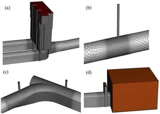
Figure 2. Mesh division of key areas in the tailrace system: (a) surge chamber, (b) air vent 1#, (c) the tailrace–diversion junction, and (d) tailwater.

2.4. Computational Scenarios and Boundary Conditions

Three operating scenarios were selected to represent typical transient processes in the hydropower station, as summarized in Table 1. The S1 scenario, a complex combined condition, was used for model verification and served as a benchmark to compare results from the one-dimensional (1D) method of characteristics and three-dimensional (3D) CFD simulations. The S2 scenario corresponds to load acceptance under high tailwater conditions, where generating units gradually increase from no-load to rated load, representing a typical load rise transient. In contrast, the S3 scenario represents load rejection under high tailwater conditions, with generating units rapidly shutting down from rated load. These two scenarios are critical for assessing pressure fluctuations and air–water interactions during transient events.

Table 1. Computational scenarios of the hydropower station.

Scenarios	Upstream Water Level (m)	Tailwater Level (m)	Load Transition Pattern	Description
S1	2980.13	2759.13	1 → 2 → 0	One unit operates at rated load while the other increases from no-load; both units undergo simultaneous load rejection.
S2	2990.00	2767.45	0 → 2	Both units increase load simultaneously from no-load to rated conditions.
S3	2991.00	2768.69	2 → 0	Two units undergo simultaneous load rejection from rated operation.

In this study, ANSYS Fluent 2022 software, coupled with a high-performance computing platform, was used for simulations. Fluent is widely utilized for simulating fluid flow in complex geometries, offering mesh adaptivity for high-precision solutions. It also provides a user-defined function (UDF) for customized development based on specific simulation requirements. The integration of the high-performance computing platform greatly enhanced both computational speed and accuracy, enabling efficient handling of complex simulations.

The computational process for transient conditions was divided into steady-state and unsteady-state simulations. In the steady-state simulation, a mass flow inlet boundary was used to determine the inlet flow at the tailrace pipe. For example, in case S1, the flow rates at the two tailrace pipe outlets were 371.89 m³/s and 21.96 m³/s, respectively. Pressure outlet boundary conditions were applied at the air vents and surge chamber, while an open-channel boundary condition was set for the downstream reservoir. The model’s key feature is its ability to simulate free-surface flow, where the fluid surface is unconstrained and can fluctuate freely. The gravitational effects on the fluid were fully accounted for, making the model well-suited for simulating reservoir water levels. In case S1, the tailwater elevation was 2759.13 m, the bottom elevation was 2751 m, and the water depth was 8.13 m, with the air–water interface shown in Figure 3a.

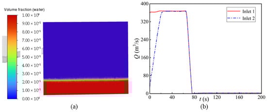
Figure 3. Boundary conditions: (a) air–water interface diagram of the downstream reservoir water level; (b) variation in flow rate at the tailrace pipe inlet.

In the unsteady-state simulation, the mass flow inlet boundary was also applied. The flow rate variation curve, obtained using the MOC method, was introduced into the tailrace pipe inlet through UDF. As shown in Figure 3b, this UDF captures dynamic flow variations. The time step for the simulation was set to 0.025 s, allowing for the capture of free-surface motion and transient pressure variations throughout the process.

3. Results and Discussion

3.1. Numerical Validation and Surge Oscillation Analysis

The water-level fluctuation process of the surge chamber under operating condition S1 is shown in Figure 4, and the comparison of the initial, maximum, and minimum water levels between the 1D and 3D simulations is summarized in Table 2. The results indicate that the overall variation trends obtained by the one-dimensional and three-dimensional models are highly consistent. The initial water levels predicted by the two models differ by only 0.22 m, while the peak and trough water levels differ by less than 0.25 m, corresponding to a relative deviation of less than 0.01%. These results verify that the CFD model accurately reproduces the unsteady surge oscillations obtained by the 1D method of characteristics, demonstrating its capability to capture both the amplitude and phase of the water-level fluctuation with high fidelity. The close agreement between the two approaches confirms the reliability of the numerical framework used in this study. This comparison between the 1D MOC model and the 3D CFD simulations serves as a preliminary numerical verification of the applied modeling framework.

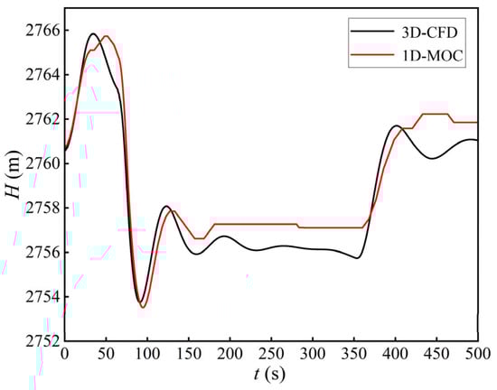
Figure 4. Water-level fluctuation process of the surge chamber.

Table 2. Comparison of surge chamber water levels between 1D and 3D simulations.

Simulation Method	Initial Water Level (m)	Maximum Water Level (m)	Minimum Water Level (m)
1D-MOC	2760.75	2765.70	2753.51
3D-CFD	2760.53	2765.83	2753.74

3.2. Sensitivity Analysis of Vent Number and Diameter

3.2.1. Air-Vent Layout Scheme Description

Based on the preliminary design of the large-scale diversion system at the hydropower station, six distinct air-vent layout configurations were proposed, varying in the number and diameter of the air vents. These configurations were designed to improve hydraulic stability while minimizing construction costs. In the reference project, the locations of vents 1#–4# were determined based on geological conditions, structural feasibility, and practical engineering experience. These positions were therefore adopted as the baseline vent layout (Type 1), and the alternative configurations (Types 2–6) were subsequently developed through sensitivity analyses on vent number and diameter. Given the representative nature of the selected operating conditions, transient characteristics were analyzed under both load acceptance and load rejection scenarios. The analysis focused on pressure fluctuations at the tailrace–diversion junction, the intake and exhaust air velocities for each vent, and the variations in surge water levels within the surge chamber. The details of these six configurations are summarized in Table 3, with the 3D model of each layout shown in Figure 5.

Table 3. Air-vent layout schemes.

Type	Number of Air Vents	Diameter of Air Vents (m)	Description
Type 1	4	2	Air vents 1#, 2#, 3#, 4#
Type 2	3	2	Air vents 2#, 3#, 4#
Type 3	2	2	Air vents 3#, 4#
Type 4	1	2	Air vent 4#
Type 5	1	2	Air vent 5#
Type 6	1	3	Air vent 6#

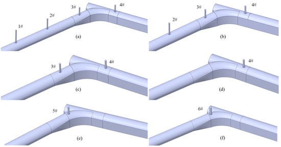
Figure 5. 3D models of air-vent layout schemes: (a) Type 1, (b) Type 2, (c) Type 3, (d) Type 4, (e) Type 5, and (f) Type 6.

3.2.2. Load Acceptance Condition

The transient calculation results for the tailrace system under the six different air-vent configurations are summarized in Table 4. The analysis focuses on three main parameters: the pressure fluctuations at the tailrace–diversion junction (point up1), the maximum intake/exhaust air velocities for each vent, and the surge water level variations in the surge chamber. The simulation results indicate that, with the implementation of air vents, the negative pressure at the junction is significantly reduced, confirming the effectiveness of venting in mitigating transient pressure fluctuations.

Table 4. Calculation results for different air-vent layouts.

Type	Minimum Pressure at Junction (m)	Maximum Intake/Exhaust Air Velocity (m/s)					Surge Water Level (m)
		1#	2#	3#	4#	5#/6#	Maximum	Minimum
1	−1.37	1.90/−3.29	2.34/−3.78	50.84/−4.99	60.98/−79.69	/	2783.48	2765.04
2	−1.06	/	1.99/−3.18	50.76/−3.50	64.86/−84.64	/	2783.32	2765.01
3	−1.35	/	/	54.19/−2.06	76.83/−49.60	/	2783.55	2764.96
4	−2.289	/	/	/	97.38/−78.05	/	2783.54	2764.85
5	−0.66	/	/	/	/	90.02/−67.17	2783.54	2764.88
6	−0.14	/	/	/	/	43.49/−13.29	2783.50	2765.24

When no air vents were placed at the junction, the CFD simulations revealed that the tailrace system experienced a severe negative pressure of −12.15 m at the junction due to the long diversion tunnel and the inertial effects of the water. This could potentially cause column separation, indicating the necessity of air-vent installation. As shown in Figure 6, the pressure fluctuation curves at the tailrace–diversion junction across the six configurations are generally similar, with notable differences in the lowest pressure point between 50 and 150 s. Specifically, Configuration 6, with a larger vent diameter, showed the most moderate negative pressure, demonstrating that increasing the vent diameter improves the pressure regulation significantly. Interestingly, configurations with more vents did not lead to better negative pressure mitigation; instead, reducing the number of vents while increasing their diameter (as seen in Type 6) was more effective.

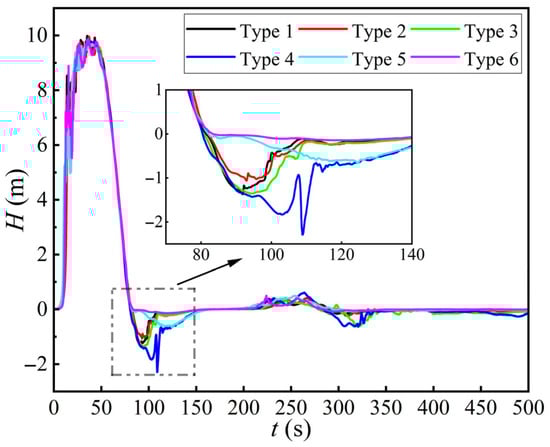
Figure 6. Pressure fluctuations at the tailrace–diversion junction (S2).

The direction of air velocity for vents 1#–4# is defined as positive for intake and negative for exhaust. In configurations Type 1–3, the intake/exhaust air velocities at vents 1# and 2# were near 0 m/s, suggesting that water immersion occurred at these vents, diminishing their effectiveness. In contrast, configurations with a single vent (Type 4–6) exhibited more significant air velocity values, with Type 6 showing the most substantial improvement in airflow. Specifically, the intake air velocity in Type 6 decreased by 43.39%, and the exhaust velocity decreased by 73.20%, indicating a marked improvement in air-vent performance due to the larger vent diameter.

As shown in Figure 7, the surge water level fluctuations in the surge chamber were similar across all six configurations, with minimal differences in the maximum and minimum surge water levels. The differences in surge levels were within 0.5 m, which is attributed to the interplay of mixed-flow phenomena at the tailrace–diversion junction and the superimposed fluctuations. Overall, the air-vent configurations had minimal impact on surge water level fluctuations, suggesting that the main benefit of the air-vent installation is its effect on pressure regulation rather than surge damping.

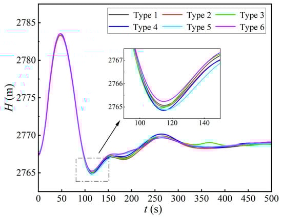
Figure 7. Water level fluctuations in the surge chamber (S2).

Therefore, the analysis demonstrates that the number and size of air vents, as well as their placement, significantly influence the system’s transient hydraulic performance. Increasing the vent diameter, particularly to 3 m, as seen in Type 6, optimizes pressure regulation and air exchange efficiency, ensuring more stable operation. However, increasing the number of vents does not necessarily improve hydraulic performance, underscoring the importance of strategic placement and sizing of the vents.

To better understand the complex hydraulic phenomena during the mixed-flow process, particularly the impact of air-vent configuration on the tailrace system, the transient behavior of the air–water interface and surge water levels was analyzed. This analysis primarily focuses on the air–water interaction at the tailrace–diversion junction, as shown in Figure 8, along with the changes in water levels within the surge chamber.

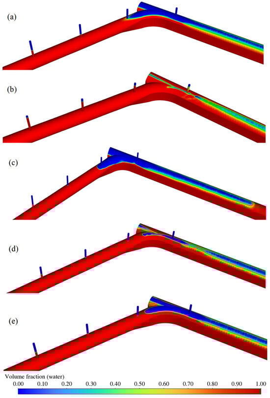
Figure 8. Air–water distribution at the tailrace–diversion junction during the transient process: (a) t = 0 s, (b) t = 49.50 s, (c) t = 113.72 s, (d) t = 268.80 s, and (e) t = 450.00 s.

At the beginning of the simulation (t = 0 s), during the steady-state condition, air vents 1# and 2# are submerged in water, corresponding to near-zero air velocity, indicating the presence of water flow. Vent 3# is at the interface between the air and water phases, where the exhaust velocity approaches zero, and vent 4# remains out of the submerged zone, showing relatively high intake and exhaust air velocities. As the hydropower unit begins to load (t = 0–49.50 s), the flow rate increases, causing the surge chamber water level to rise and the air vents to enter the exhaust phase. By t = 49.50 s, the surge chamber reaches its maximum water level of 2783.48 m, as shown in Figure 8b. During this time, the water level rises in all vents, with vent 4# approaching its top due to the inertial effects, causing almost complete submersion at the tailrace–diversion junction. From t = 49.50 s to 113.72s, with the unit’s flow stabilized, the inertia of the water continues to push downstream, causing the surge chamber water level to drop to a minimum of 2765.04 m. As seen in Figure 8c, vents 1# and 2# remain submerged, while vents 3# and 4# emerge, indicating a shift to intake, and the water level in these vents decreases. The water hammer continues to propagate downstream. From t = 113.72 s to 268.80 s, the inertia of the water in the tailrace pipe keeps moving towards the surge chamber, while the pressure wave continues its travel downstream. As the diversion tunnel is significantly longer than the tailrace pipe, the pressure wave in the diversion tunnel has not yet reached the downstream reservoir by the time the water flow from the tailrace pipe reaches the surge chamber, avoiding the wave reflection. At t = 268.80 s, the complex interaction between the inertia wave in the tailrace pipe and the reflected wave in the diversion tunnel results in the maximum surge water level. The combination of wave propagation and superposition continues to influence the system until t = 450 s, when the system approaches a stable state.

This entire transition process, involving the tailrace tunnel, diversion tunnel, and the junction section, showcases the complex interactions of different types of hydraulic waves. These results highlight the importance of optimizing the air-vent configurations to mitigate transient effects, manage pressure fluctuations, and improve system stability.

3.2.3. Load Rejection Condition

To further validate the computational scheme, a detailed comparison and analysis of different air-vent layout configurations and their diameters were conducted under the load rejection condition (S3). The results are summarized in Table 5, with transient variations in pressure fluctuations at the tailrace–diversion junction under S3 presented in Figure 9, and surge water level fluctuations in the surge chamber shown in Figure 10. The analysis indicates significant improvements with Type 6, featuring a single air vent with a diameter of 3 m, placed near the downstream section of the tailrace junction’s starting area.

Table 5. Calculation results for different air-vent layouts (S3).

Type	Minimum Pressure at Junction (m)	Maximum Intake/Exhaust Air Velocity (m/s)					Surge Water Level (m)
		1#	2#	3#	4#	5#/6#	Maximum	Minimum
5	−3.12	/	/	/	118.0/−82.78	/	2773.78	2757.48
6	−0.76	/	/	/	/	98.30/−52.62	2775.18	2758.52

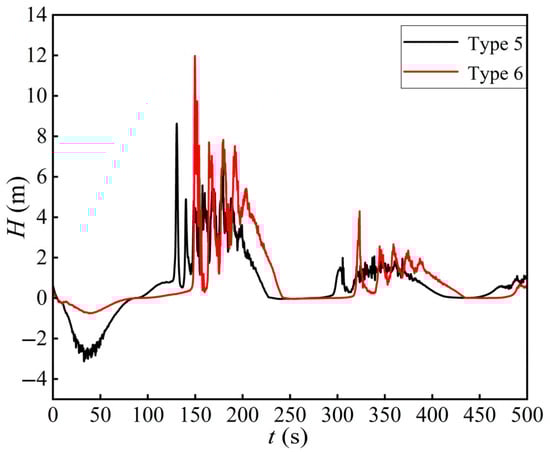
Figure 9. Pressure fluctuations at the tailrace–diversion junction (S3).

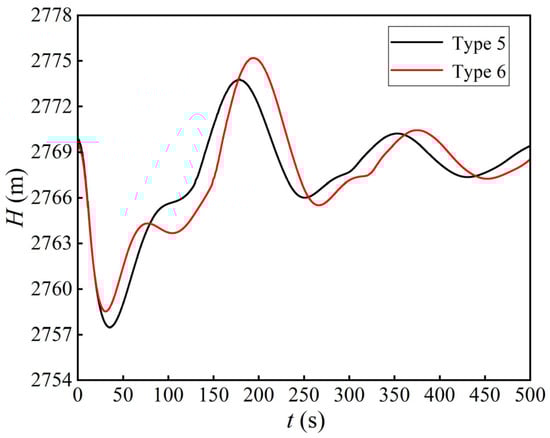
Figure 10. Surge water level fluctuations in the surge chamber (S3).

Although Type 5 presents smaller pressure fluctuations in some localized periods, the negative pressure at the tailrace–diversion junction is the critical safety parameter. As indicated by Table 5 and Figure 9, Type 6 yields a milder negative-pressure response during the key 0–100 s interval and reduces peak intake/exhaust air velocities. Consequently, Type 6 demonstrates a more stable and safer transient behavior than Type 5.

3.3. Sensitivity Analysis of Vent Height

3.3.1. Monitoring Setup and Research Necessity

To investigate the influence of vent geometry on transient hydraulic behavior, a sensitivity analysis was conducted for various vent heights under the S2 load-acceptance condition. This scenario was selected because prior simulations indicated that the highest downstream tailwater level, combined with rapid flow acceleration during load acceptance, may cause potential overflow from the vent shaft, as shown in Figure 8b.

The initial vent height was set to 12 m, measured from the crown of the tunnel to the top of the vent, with a vent diameter of 3 m. The center of the vent was positioned 3 m downstream from the transition section. Four different vent heights were evaluated: 12 m, 13 m, 15 m, and 22 m, to assess the impact of vent height on transient flow characteristics and vent performance. Two monitoring approaches were used to comprehensively assess the transient water level within the vent:

Method I: Monitors the total pressure head at the vent’s bottom section, which is converted into the equivalent water level to capture the hydraulic response during transient conditions.

Method II: Tracks the two-phase interface position (with a volume fraction of 0.5) to determine the water–air interface height during the maximum rise in the water level.

The use of these complementary methods is crucial. Method I provides insights into the overall pressure response at the base, which is linked to potential pressurized flow and vent discharge. Method II, on the other hand, offers valuable information on free-surface deformation and jet behavior, phenomena that are difficult to capture using pressure measurements alone.

3.3.2. Hydraulic Transient Response

The transient pressure fluctuation process at the bottom of the air vent under the four different configurations is shown in Figure 11, based on the monitoring method I. The results indicate that the pressure fluctuation trends and peak values are largely consistent across the four configurations, with only slight differences observed in the maximum values. Specifically, the peak water head occurs at approximately t = 35 s, with values ranging between 9.30 m and 9.60 m, showing a deviation of less than 0.3 m.

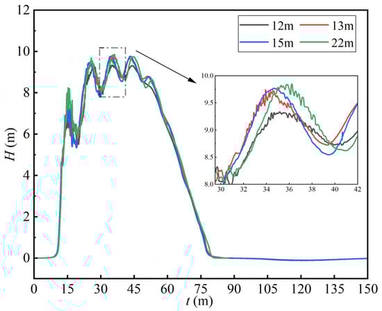
Figure 11. Pressure head fluctuations under different vent heights.

At t = 35 s, the pressure distribution at the vent bottom is shown in Figure 12. The maximum pressure is observed during the surge water level rise phase in the surge chamber, with the highest pressure located near the junction of the tailrace and diversion tunnel. The location of the maximum pressure remains similar across all four configurations. The results suggest that the vent height has minimal impact on the base hydraulic head or the overall transient response of the system.

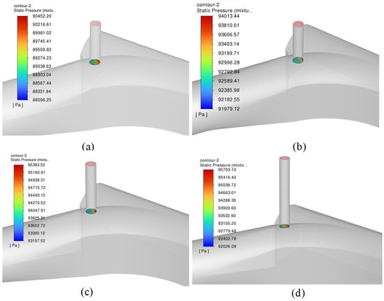
Figure 12. Pressure distribution at the vent bottom for different vent heights (t = 35 s): (a) vent height 12 m, (b) vent height 13 m, (c) vent height 15 m, and (d) vent height 22 m.

In contrast, Method II (VOF interface) reveals the air–water interface within the air vents, which Method I cannot capture. As shown in Figure 13, by reading the coordinates of the air–water interface nodes, the elevation of the interface can be determined, as summarized in Table 6. For vents with a height of 12 m and 13 m, the interface briefly reaches the top of the vent, indicating a minor risk of overflow. In contrast, for vents with heights of 15 m and 22 m, the maximum interface elevations are 13.29 m and 13.67 m, respectively, maintaining a freeboard of 1.71 m and 8.33 m, effectively preventing water overflow.

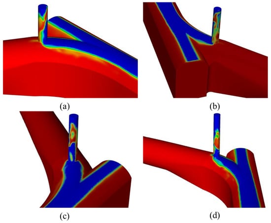
Figure 13. Air–water interface distribution for different vent heights (t = 35 s): (a) vent height 12 m, (b) vent height 13 m, (c) vent height 15 m, and (d) vent height 22 m.

Table 6. Maximum water levels under different vent heights (35 s).

Case	Vent Height (m)	Peak Water Level (m)	VOF Interface Elevation (m)	Description
1	12	9.30	Slight overflow	Initial vent height 12 m
2	13	9.60	Minor overflow	Vent height 13 m
3	15	9.30	13.29	Vent height 15 m
4	22	9.49	13.67	Vent height 22 m

In the configurations with adequate freeboard (case 3 and case 4), the air–water interface remained between 13.30 m and 13.70 m, with a deviation of approximately 0.4 m. This suggests that the effect of vent height on water level is minimal, and as long as there is sufficient freeboard (e.g., with Type 3, where the vent height is 15 m), overflow can be effectively controlled. This ensures the safe and stable operation of the hydropower station.

To determine the appropriate vent height, we recommend a practical clearance rule. Based on the transient analysis and the observed maximum air–water interface elevation of approximately 13.7 m, the vent height should be selected using the following criterion:

$$H_{vent}\ge H_{IF,\max }+\Delta h$$

(8)

where H_IF,max is the water–air interface elevation observed during the transient (here ≈ 13.7 m), and $\Delta h$ is the safety allowance; 1–2 m is recommended to account for modeling uncertainties, construction tolerances, and operational variability.

During load acceptance, an inertia-driven surge propagates through the long tailrace–diversion system. When the incoming surge interacts constructively with the reflected wave at the junction, the free surface rises sharply, forming a short-lived vertical jet along the back wall of the vent. This process alternates between free-surface and pressurized flow states within the shaft. Because Method I integrates the sectional pressure response, it is less sensitive to these localized, rapid jet fluctuations, hence the narrow range of 9.30–9.60 m across all vent heights. In contrast, the VOF interface directly captures the transient surface excursion and splash, which are critical for assessing overflow risk. The VOF threshold at a volume fraction of 0.5 provides a conservative yet practical estimate of the peak water surface, offering a reliable upper bound for design.

4. Discussion

This study examines the impact of air-vent configurations on the transient hydraulic behavior of the tailrace system in a hydropower station, aiming to optimize the vent layout for improved system stability and mitigation of transient effects, such as pressure fluctuations and overflow risks. A combination of 1D and 3D numerical models was employed to analyze the transient characteristics under both load acceptance and load rejection conditions, testing various air-vent configurations.

The results show that increasing the vent diameter, particularly to 3 m as seen in Type 6, greatly improves pressure regulation and air exchange efficiency, leading to enhanced system stability.

The larger-diameter vent performs better because its reduced air-flow resistance and smaller air–column inertia allow air exchange to occur under a smaller pressure gradient, thereby suppressing extreme negative pressures at the junction. Increasing the number of vents provides limited additional benefit, as the dominant transient pressure wave is concentrated near the junction, while vents located in regions with weak pressure gradients contribute little and may introduce additional frictional and inertial losses.

Unlike increasing the number of vents, enlarging the vent diameter has a more significant impact on system performance by reducing negative pressure and maintaining smoother operation during transient conditions. Additionally, the positioning of the air vent is crucial; placing the vent near the downstream end of the tailrace junction minimizes negative pressure fluctuations and reduces the risk of overflow.

Sensitivity analysis on vent height reveals that increasing the height from 12 m to 15 m improves system stability by providing sufficient freeboard, while further increasing the height to 22 m results in diminishing returns. This highlights that vent height does influence transient flow characteristics, but it is the combination of optimal vent diameter and strategic placement that most effectively addresses transient overflow and pressure fluctuations.

5. Conclusions

This study introduces a three-dimensional (3D) computational framework, coupled with MOC boundary conditions, to investigate transient hydraulic behavior and optimize air-vent configurations in a combined draft–tailrace system. The 1D model provides precise discharge for boundary conditions, while the 3D CFD model, employing the Volume of Fluid (VOF) method, effectively captures localized air–water interactions and transient pressure fluctuations. This integrated approach simulates both large-scale flow oscillations and fine-scale interface dynamics, enabling a quantitative assessment of vent geometry under transient operating conditions.

• The comparison between the 1D and 3D simulations shows excellent agreement in predicting surge chamber oscillations, with deviations in maximum and minimum water levels of less than 0.3%. The 3D model successfully replicates transitions between free-surface and pressurized flow, as well as the air–water interface deformation during transient events, confirming its ability to accurately assess mixed-flow behavior and hydraulic risks in long tailrace systems.
• Analysis under both load acceptance and load rejection conditions indicates that increasing the number of vents does not necessarily improve hydraulic stability. Instead, enlarging the vent diameter significantly enhances air exchange efficiency and pressure regulation. The optimal configuration, featuring a single 3 m diameter vent located near the downstream end of the junction, provides the best overall performance, reducing negative pressure, suppressing peak velocities, and maintaining stable surge levels with minimal construction complexity.
• Sensitivity analysis reveals that while vent height has minimal impact on overall pressure head, it significantly affects the risk of transient overflow. Increasing vent height from 12 m to 15 m ensures approximately 1.7 m of freeboard during high-water-level load acceptance, preventing overflow while avoiding excessive structural elevation. A design criterion is proposed: the vent height should exceed the maximum observed air–water interface elevation by 1–2 m to ensure operational safety.

References

- Hassan, Q.; Algburi, S.; Sameen, A.Z.; Al-Musawi, T.J.; Al-Jiboory, A.K.; Salman, H.M.; Ali, B.M.; Jaszczur, M. A Comprehensive Review of International Renewable Energy Growth. Energy Built Environ. 2024, in press. [Google Scholar] [CrossRef]
- Man, X.; Song, H.; Li, H. Estimating Hydropower Generation Flexibilities of a Hybrid Hydro–Wind Power System: From the Perspective of Multi-Time Scales. Energies 2023, 16, 5218. [Google Scholar] [CrossRef]
- Xu, J.; Ni, T.; Zheng, B. Hydropower Development Trends from a Technological Paradigm Perspective. Energy Convers. Manag. 2015, 90, 195–206. [Google Scholar] [CrossRef]
- Guo, W.; Zhu, D. Critical Stable Sectional Area of Downstream Surge Tank of Hydropower Plant with Sloping Ceiling Tailrace Tunnel. Energy Sci. Eng. 2021, 9, 1090–1102. [Google Scholar] [CrossRef]
- Kemarau, R.A.; Harun, S.N.; Sa’adi, Z.; Mohd Hanafiah, M.; Sakawi, Z.; Norzin, M.A.F.; Wan Mohd Jaafar, W.S.; Anak Suab, S.; Eboy, O.V.; Abdul Maulud, K.N. Transforming Hydropower: An in-Depth Systematic Review of Climate Change Impacts. Renew. Sustain. Energy Rev. 2025, 219, 115890. [Google Scholar] [CrossRef]
- Liu, Y.; Yu, X.; Guo, X.; Zhao, W.; Chen, S. Operational Stability of Hydropower Plant with Upstream and Downstream Surge Chambers during Small Load Disturbance. Energies 2023, 16, 4517. [Google Scholar] [CrossRef]
- Zhong, Z.; Zhu, L.; Zhao, M.; Qin, J.; Zhang, S.; Chen, X. Stability and Sensitivity Characteristic Analysis for the Hydropower Unit Considering the Sloping Roof Tailrace Tunnel and Coupling Effect of the Power Grid. Front. Energy Res. 2023, 11, 1242352. [Google Scholar] [CrossRef]
- Xu, P.; Fu, W.; Lu, Q.; Zhang, S.; Wang, R.; Meng, J. Stability Analysis of Hydro-Turbine Governing System with Sloping Ceiling Tailrace Tunnel and Upstream Surge Tank Considering Nonlinear Hydro-Turbine Characteristics. Renew. Energy 2023, 210, 556–574. [Google Scholar] [CrossRef]
- Zhou, D.; Chen, H.; Chen, S. Research on Hydraulic Characteristics in Diversion Pipelines under a Load Rejection Process of a PSH Station. Water 2019, 11, 44. [Google Scholar] [CrossRef]
- Ling, L.; Jiandong, Y.; Meiqing, L. Study on the Disruption of Water Flow in the System of Tailrace Tunnel Combined with Diversion Tunnel. IOP Conf. Ser. Earth Environ. Sci. 2014, 22, 042005. [Google Scholar] [CrossRef]
- Li, G.; Zhou, T.; Zhang, W.; Yang, F. Influence of mixed free-surface and pressurized flow on transient process in a tailrace tunnel of a tailrace surge chamber. IOP Conf. Ser. Earth Environ. Sci. 2021, 826, 012008. [Google Scholar] [CrossRef]
- Guo, W. A Review of the Hydraulic Transient and Dynamic Behavior of Hydropower Plants with Sloping Ceiling Tailrace Tunnels. Energies 2019, 12, 3220. [Google Scholar] [CrossRef]
- Bergant, A.; Simpson, A.R.; Tijsseling, A.S. Water Hammer with Column Separation: A Historical Review. J. Fluids Struct. 2006, 22, 135–171. [Google Scholar] [CrossRef]
- Adamkowski, A.; Lewandowski, M. Investigation of Hydraulic Transients in a Pipeline with Column Separation. J. Hydraul. Eng. 2012, 138, 935–944. [Google Scholar] [CrossRef]
- Zhou, J.; Mao, Y.; Shen, A.; Zhang, J. Modeling and stability investigation on the governor-turbine-hydraulic system with a ceiling-sloping tail tunnel. Renew. Energy 2023, 204, 812–822. [Google Scholar] [CrossRef]
- Guo, J.; Zhou, D.; Wang, H. Study of Intermittent Jets and Free-Surface-Pressurized Flow in Large Hydropower Tailrace Tunnel. Phys. Fluids 2024, 36, 053342. [Google Scholar] [CrossRef]
- Nomeritae, N.; HaHong, B.; Edoardo, D. Modeling Transitions between Free Surface and Pressurized Flow with Smoothed Particle Hydrodynamics. J. Hydraul. Eng.-ASCE 2018, 144, 04018012. [Google Scholar] [CrossRef]
- Zhang, J.; Chen, J.; Xu, W.; Wang, Y.; Li, G. Three-Dimensional Numerical Simulation of Aerated Flows Downstream Sudden Fall Aerator Expansion-In a Tunnel. J. Hydrodyn. 2011, 23, 71–80. [Google Scholar] [CrossRef]
- Cheng, Y.; Li, J.; Yang, J. Free Surface-Pressurized Flow in Ceiling-Sloping Tailrace Tunnel of Hydropower Plant: Simulation by VOF Model. J. Hydraul. Res. 2007, 45, 88–99. [Google Scholar] [CrossRef]
- Zhang, X.; Cheng, Y. Simulation of Hydraulic Transients in Hydropower Systems Using the 1-D-3-D Coupling Approach. J. Hydrodyn. 2012, 24, 595–604. [Google Scholar] [CrossRef]
- Xia, L.; Cheng, Y.; Zhou, D. 3-D simulation of transient flow patterns in a corridor-shaped air-cushion surge chamber based on computational fluid dynamics. J. Hydrodyn. Ser. B 2013, 25, 249–257. [Google Scholar] [CrossRef]
- Zhou, J.; Li, Y. Modeling of the Free-Surface-Pressurized Flow of a Hydropower System with a Flat Ceiling Tail Tunnel. Water 2020, 12, 699. [Google Scholar] [CrossRef]
- Wang, X.; Fan, H.; Liu, B. Optimization Control on the Mixed Free-Surface-Pressurized Flow in a Hydropower Station. Processes 2021, 9, 320. [Google Scholar] [CrossRef]
- Wang, C.; Yang, J.; Nilsson, H. Simulation of Water Level Fluctuations in a Hydraulic System Using a Coupled Liquid-Gas Model. Water 2015, 7, 4446–4476. [Google Scholar] [CrossRef]
- Zhang, W.; Cai, F.; Zhou, J.; Hua, Y. Experimental Investigation on Air-Water Interaction in a Hydropower Station Combining a Diversion Tunnel with a Tailrace Tunnel. Water 2017, 9, 274. [Google Scholar] [CrossRef]
- Wang, X.; Zhang, J.; Yu, X.; Chen, S. Transient Air-Water Flow Patterns in the Vent Tube in Hydropower Tailrace System Simulated by 1-D-3-D Coupling Method. J. Hydrodyn. 2018, 30, 715–721. [Google Scholar] [CrossRef]
- Chaudhry, M.H. Applied Hydraulic Transients; Springer: New York, NY, USA, 2014; ISBN 978-1-4614-8537-7. [Google Scholar]
- Mulbah, C.; Kang, C.; Mao, N.; Zhang, W.; Shaikh, A.R.; Teng, S. A Review of VOF Methods for Simulating Bubble Dynamics. Prog. Nucl. Energy 2022, 154, 104478. [Google Scholar] [CrossRef]
Disclaimer/Publisher’s Note: The statements, opinions and data contained in all publications are solely those of the individual author(s) and contributor(s) and not of MDPI and/or the editor(s). MDPI and/or the editor(s) disclaim responsibility for any injury to people or property resulting from any ideas, methods, instructions or products referred to in the content. |
© 2025 by the authors. Licensee MDPI, Basel, Switzerland. This article is an open access article distributed under the terms and conditions of the Creative Commons Attribution (CC BY) license (https://creativecommons.org/licenses/by/4.0/).