Quality Performance Criterion Model for Distributed Automated Control Systems Based on Markov Processes for Smart Grid

Abstract

This paper addresses the problem of decision-making support for the modernization of distributed automated control systems (ACS) in power engineering by proposing an integral quality criterion that combines similarity-driven Markov process modeling with geometric programming. The methodology transforms the transition rate matrix of a continuous-time Markov chain (CTMC) into a matrix polynomial, enabling the derivation of normalized similarity indices and the development of a criterion-based model to quantify relative variations in system quality without requiring global optimization. The proposed approach yields a generalized criterion model that facilitates the ranking of modernization alternatives and the evaluation of the sensitivity of optimal decisions to parameter variations. The practical implementation is demonstrated through updated state transition graphs, quality functions, and UML-based architectures of diagnostic-ready evaluation modules. The scientific contribution of this work lies in the integration of similarity-based Markov modeling with the mathematical framework of geometric programming into a unified criterion model for the quantitative assessment of functional readiness under multistate conditions and probabilistic failures. The methodology enables the comparison of modernization scenarios using a unified integral indicator, assessment of sensitivity to structural and parametric changes, and seamless integration of quality evaluation into SCADA/Smart Grid environments as part of real-time diagnostics. The accuracy of the assessment depends on the adequacy of transition rate identification and the validity of the Markovian assumption. Future extensions include the real-time estimation of transition rates from event streams, generalization to semi-Markov processes, and multicriteria optimization considering cost, risk, and readiness.

1. Introduction

Modern automated control systems (ACS) in the power sector are characterized by distributed, multi-level architectures and operate under continuous variations in external load, network disturbances, and the integration of Smart Grid components. This inherent complexity increases the likelihood of state transitions and complicates the quantitative assessment of functional readiness during both operation and modernization. Traditional reliability assessment methods typically rely on deterministic indicators or require precise knowledge of optimal parameters, which significantly complicates decision making in multi-scenario modernization tasks [1,2].

In this study, we combine the apparatus of Markov processes with similarity theory and criterion-based modeling to construct an integral quality index for ACS performance. Applying matrix polynomials to the transition rate matrix enables the derivation of normalized similarity criteria, while the subsequent application of geometric programming provides the means to evaluate relative quality variations without the explicit search for global optima. The objective of the article is to develop a methodology for forming an integral performance indicator and to demonstrate its applicability to ACS modernization decision making.

1.1. Novelty and Practical Significance

The proposed criterion-based model integrates similarity-driven Markov process modeling with geometric programming for ACS quality evaluation. A normalized integral indicator is introduced, suitable for ranking modernization alternatives. UML models of diagnostic-ready modules are presented to facilitate the practical implementation of assessment algorithms and visualization of results. Furthermore, algorithmic methods are developed to combine continuous-time Markov chains (CTMC) with geometric programming through normalized similarity criteria. The approach enables the processing of telemetry data, ranking of alternatives, and formulation of rigorous conditions, demonstrating the advantages of normalization over conventional optimization in functional reliability evaluation. Mathematical statements (Lemma and Theorem) and an experimental design plan provide additional formal grounding and application validation [3,4,5].

Due to their distributed structure, ACS can continue performing their functions in the event of component failures, albeit with reduced efficiency. This implies the presence of multiple operational states, which necessitates a performance indicator that quantifies the system’s ability to accomplish its functions and its degree of readiness—directly affecting the optimal state of the controlled object. Such an indicator is the functional quality of the ACS [5]. Importantly, this metric should characterize the ACS over a given time interval during which its operability varies but remains within permissible limits. In other words, it must be integral in nature and represent all operational states collectively.

A common feature across all operational states of an ACS is that its defining parameters and their ratios ensure system performance within the domain of optimality. Therefore, to analyze ACS functionality in an optimal control context, it is necessary to substitute it with a similarity-based model whose properties are proportional to those of the original system.

Accordingly, the contribution of this work lies in unifying established methods—CTMC and geometric programming (GP)—into a coherent procedure, formalizing the methodological steps, and demonstrating their practical application for ACS.

1.2. Similarity-Based Markov Process Modeling

Markov processes form the foundation of the proposed approach, enabling the formalization of the multistate behavior of automated control systems (ACS) in terms of transitions between states with associated intensities. Due to the memoryless property of Markov chains, the system can be represented by a compact generator matrix Q, which ensures mathematical rigor, the possibility of analytical solutions, and the applicability of numerical methods to complex structures. This representation makes it possible not only to determine the probabilities of the system being in nominal, degraded, or failed states but also to integrate additional quality criteria based on the similarity indices (π_i), dual functionals (d*(p*)), and integral measures (S).

The potential applications of similarity-based modeling are multidimensional. First, it provides the basis for real-time diagnostics and maintenance decision making: transition intensities can be updated dynamically from telemetry and event streams, enabling the timely detection of degradations. Second, it supports the evaluation of modernization effectiveness in energy and industrial automation systems: by comparing relative variations in quality functionals, the most feasible modernization scenarios can be identified without exhaustive enumeration. Third, in the context of Smart Grids, Markov modeling enables adequate representation of complex failures and degradations in decentralized architectures, including the integration of renewable energy sources and storage systems.

A particularly important aspect is its application to the cyber-resilience of ACS. Degraded states of communications and sensing subsystems may result from both technical faults and external cyber attacks. To address this, the model incorporates additional transitions that capture such events, thereby allowing not only the monitoring of hardware reliability but also the formation of comprehensive resilience assessments against cyber threats.

Future development of the model may proceed in several directions. First, integrating semi-Markov processes (SMP) would allow for the representation of arbitrary sojourn-time distributions, bringing the model closer to real-life degradation and maintenance dynamics. Second, combining Markov decision processes (MDP) with reinforcement learning methods establishes a foundation for optimizing operational and maintenance strategies under cost, risk, and reliability criteria. Third, the application of multi-objective optimization and geometric programming opens pathways toward balanced policies that simultaneously minimize risk and cost while maintaining target readiness levels.

Thus, Markov process modeling in the ACS context emerges not only as an analytical tool but also as a conceptual foundation for developing adaptive, self-learning, and cyber-resilient control systems that meet the contemporary challenges of digitalization, decentralization, and energy transition.

The classical Kolmogorov system of equations is expressed as

$${\displaystyle \frac{dp(\mathrm{t})}{dt}}=Q^{T}p(t),$$

where p(t) is the row vector of state probabilities, and Q is the generator matrix of the continuous-time Markov chain (CTMC).

$${\displaystyle {\sum }_j{q}_{ij}=0 ,} q_{ij}<0.$$

Thus, as is well known, a Markov process is described by a system of differential equations [3]:

$$\left.\begin{array}{l}{\displaystyle \frac{dp}{dt}}=\nu \cdot p;\\ {\displaystyle \sum _{i=1}^m{p}_i=1 ,}\end{array}\right\},$$

(1)

where p is the vector of state probabilities of the system under study; ν is the matrix of transition probability densities between states; and m is the number of possible states of the system (see Figure 1).

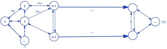
Figure 1. State transition graph of the ACS.

Analyzing the system of Equation (1), it is rather difficult to directly derive criteria that would fully satisfy the requirements. However, it can be employed to construct a similarity-based model, in which the properties, parameters, and variable values are proportional to the corresponding properties, parameters, and variables of the original system [6].

For steady-state conditions of the system ${\displaystyle \frac{\mathrm{d}{\mathrm{p}}_{\mathrm{i}}}{\mathrm{d}\mathrm{t}}}=0$ can be rewritten as

$$\left.\begin{array}{l}{\displaystyle \sum _{\mathrm{i}=1}^{\mathrm{m}}{\mathrm{\nu }}_{\mathrm{j}\mathrm{i}}{\mathrm{p}}_{\mathrm{i}}=0, \mathrm{j}=\overline{2,\mathrm{n}}}\\ {\displaystyle \sum _{\mathrm{i}=1}^{\mathrm{m}}{\mathrm{p}}_{\mathrm{i}}}=1,\end{array}\right\},$$

(2)

where the elements of the matrix ${\nu }_{ji}$ are constant values representing algebraic sums of the transition intensities from state i to state j, and n denotes the number of outgoing transitions from the operational state 1 (see Figure 1).

In a more general form, Equation (2) is written as

$$[Q^T;\cdot 1^T]p=[0;1],$$

(3)

where p is the stationary distribution, and the matrix ν from (1) is augmented by a row of m ones to enforce normalization.

To establish similarity, we construct a polynomial of the transition matrix ν., analogous to the representation of any analytic function f(x) as a convergent polynomial expansion of a scalar variable x [7]:

$$\mathrm{f}\left(\mathrm{x}\right)={\mathrm{a}}_0+{\mathrm{a}}_1\mathrm{x}+{\mathrm{a}}_2{\mathrm{x}}^2+\dots ={\displaystyle \sum _{\mathrm{s}=0}^{\infty }{\mathrm{a}}_{\mathrm{s}}{\mathrm{x}}^{\mathrm{s}}}.$$

The function of a matrix $\mathrm{f}\left(\mathrm{X}\right)$ can likewise be expressed as a matrix polynomial, formally obtained by replacing the scalar variable x with the matrix X.

$$\mathrm{f}\left(\mathrm{X}\right)={\mathrm{a}}_0+{\mathrm{a}}_1\mathrm{X}+{\mathrm{a}}_2{\mathrm{X}}^2+\dots ={\displaystyle \sum _{\mathrm{s}=0}^{\infty }{\mathrm{a}}_{\mathrm{s}}{\mathrm{X}}^{\mathrm{s}}.}$$

If an interpolation polynomial is employed, the transition matrix ν\nuν in Equation (3) can be transformed into a matrix polynomial [7]. In this study, the transition to the matrix polynomial through the interpolation of the exponential $f\left(z\right)=e^z$ is carried out without explicit introduction of the time parameter t or spectral analysis of the generator matrix Q.

Generator matrix Q, by definition, has dimension 1/time, because its elements λ_ij are intensities transitions;

• All degrees Q^j, which are included in the polynomial representation, store an agreed upon dimension, namely (1/time)^j;
• Function $f(Q)$, which approximates the exponential reflection exp (Q), is dimensionless, because matrix e^{Qt} specifies matrix probabilities transitions and has the sum of the elements in the rows equal to one;
• After normalization in expression (6), where all elements are divided by $f(Q)$, obtained indices similarities ${\pi }_i$ become dimensionless and the condition ${\displaystyle {\sum }_i{\pi }_i=1}$ guarantees their interpretation as agreed normalized weight coefficients.

As a result, coefficients a_j and corresponding polynomial terms are derived, from which normalized similarity criteria π_i are constructed under the imposed normalization condition ${\pi }_1+{\pi }_2+\dots +{\pi }_m=1$. It should be emphasized, however, that in the present formulation it is not proven that the obtained quantities are dimensionless, invariant, or physically interpretable. From the standpoint of classical similarity theory, explicit construction of П-groups with dimensional consistency and independence checks would be required, which is not demonstrated in the proposed framework.

Reference to spectral Q representation:

$$Q=V\mathrm{\Lambda }{V}^{-1}$$

The argument that everything and functions Q are given by polynomial interpolation, has an appearance as follows:

$$f(Q)=Vf(\mathrm{\Lambda })V^{-1},$$

That is, keep property zero sum rows if $f\left(0\right)=0$. It should be taken into account the clarification that the polynomial construction (5) approximates the exponent for which this property is proven.

This allows to formally justify statement about “non-violation of the characteristics of the i-generator matrices”.

If the minimal polynomial (in this case, the characteristic polynomial $\Delta \left(\mathrm{z}\right)$) consists only of linear factors $\left(\mathrm{z}-{\mathrm{z}}_{\mathrm{k}}\right)$, it is sufficient to evaluate the function $\mathrm{f}\left(\mathrm{z}\right)$ at the characteristic points ${\mathrm{z}}_1, {\mathrm{z}}_2, \dots , {\mathrm{z}}_{\mathrm{m}}$. In this case, the system of equations for the coefficients of the interpolation polynomial takes the form

$$f\left(z_k\right)=a_0+a_1{z}_k+\dots +a_{m-1}{z}_k^{m-1},$$

(4)

or, the matrix form

$$\left[\begin{array}{l}\mathrm{f}\left({\mathrm{z}}_1\right)\\ \mathrm{f}\left({\mathrm{z}}_2\right)\\ \dots \\ \mathrm{f}\left({\mathrm{z}}_{\mathrm{m}}\right)\end{array}\right]=\left[\begin{array}{l}1 {\mathrm{z}}_1 {\mathrm{z}}_1^2 \dots {\mathrm{z}}_1^{\mathrm{m}-1}\\ 1 {\mathrm{z}}_2 {\mathrm{z}}_2^2 \dots {\mathrm{z}}_2^{\mathrm{m}-1}\\ \dots \dots \dots \dots \dots \\ 1 {\mathrm{z}}_{\mathrm{m}} {\mathrm{z}}_{\mathrm{m}}^2 \dots {\mathrm{z}}_{\mathrm{m}}^{\mathrm{m}-1}\end{array}\right]\cdot \left[\begin{array}{l}{\mathrm{a}}_0\\ {\mathrm{a}}_1\\ \dots \\ {\mathrm{a}}_{\mathrm{m}-1}\end{array}\right].$$

By solving this system with respect to the coefficients ${\mathrm{a}}_0,{\mathrm{a}}_1,\dots , {\mathrm{a}}_{\mathrm{m}-1}$, we obtain a polynomial of the form

$$f(\nu )={\displaystyle \sum _{i=1}^m{a}_i{\displaystyle \prod _{j=1}^n}{x}_j^{{\nu }_{ji}}}.$$

(5)

By applying this transformation, all properties and consequences of similarity theory can be utilized, since it does not violate the fundamental characteristics of the generator matrix. Specifically, it is based on the spectral representation of Q and preserves the normalization condition (row sums equal zero and diagonal entries are negative) [6]. To derive the system of similarity criteria, we divide both the left- and right-hand sides of Equation (5) by f(ν):

$$1={\displaystyle \frac{a_1{\displaystyle \prod _{j=1}^n{x}_j^{{\nu }_{j1}}}}{f(\nu )}}+{\displaystyle \frac{a_2{\displaystyle \prod _{j=1}^n{x}_j^{{\nu }_{j2}}}}{f(\nu )}}+\dots +{\displaystyle \frac{a_m{\displaystyle \prod _{j=1}^n{x}_j^{{\nu }_{jm}}}}{f(\nu )}},$$

(6)

where ${\pi }_{\mathsf{i}}={\displaystyle \frac{a_i{\displaystyle \prod _{j=1}^n{x}_j^{{\nu }_{ji}}}}{f(\nu )}}=idem$, $i=\overline{1,m}$ is the similarity criteria, defined through integral analogs.

Taking into account the introduced notation for the similarity criteria, Equation (6) can be rewritten as

$${\pi }_1+{\pi }_2+\dots +{\pi }_m=1.$$

(7)

where π_i represent the normalized similarity indices, each reflecting the relative contribution of the corresponding polynomial term.

Short spectral analysis matrix Q, showing that for the representation

$$Q=V\mathrm{\Lambda }{V}^{-1},$$

any function $f\left(Q\right)$, in particular the one that used in (5)–(7), acquires the appearance

$$f(Q)=Vf(\mathrm{\Lambda })V^{-1},$$

and therefore are normalized. The indices π_i depend only on the spectrum Λ, and not on the choice of basis. In addition, what normalization (6) will provide is

$${\pi }_i(Q)={\pi }_i(SQ{S}^{-1}),$$

That is, π_i are normalized, dimensionless indices of the weight contribution of polynomial components, which reflect the structure of Markov chain transitions, are consistent with eigenvalues, and ensure invariance due to normalization.

In Equations (6) and (7), the values of the similarity criteria π_i are normalized. They represent the relative contribution of each term in Equation (5). This is equivalent to the probability of the system being in the i-th state within f(ν), which characterizes the system as a whole. Analogously, in Equation (7), the probabilities of the system states p_i obtained in Equation (1) are also normalized. This analogy allows the application of the principles of the criterion-based method, enabling the transition from solving the system of Equation (2) to analyzing system performance through criterion-based dependencies, with the optimal control state adopted as the baseline [6]. To achieve this, it is necessary to construct a criterion-based model of the Markov process.

Therefore, Equations (5)–(7) in the presented form should be interpreted primarily as a heuristic approach to normalization and ranking, rather than as a rigorous result of similarity theory. To strengthen the mathematical soundness of the formulation, it would be appropriate to complement the exposition with the spectral analysis of the generator matrix Q and explicit proofs of the invariance of the obtained similarity criteria.

1.3. Criterion-Based Model of the Markov Process

In practice, when the modernization problem of ACS is inherently multi-scenario and predominantly optimization-oriented, the obtained relation (7), which establishes similarity between Markov processes, is of limited applicability. In multi-scenario tasks, the evaluation of alternatives is typically carried out relative to a baseline scenario, which is characterized by a set of parameter values f_b, x_1b, x_2b, …, x_nb. These baseline parameters, similar to Equation (5), are linked by the condition

$$f_b(\nu )={\displaystyle \sum _{i=1}^m{a}_i{\displaystyle \prod _{j=1}^n}{x}_{jb}^{{\nu }_{ji}}}.$$

where f_b is the functional value of the baseline configuration, and x_jb denotes the baseline parameter values associated with the criterion model.

The similarity criteria for this case take the form

$${\pi }_{\mathrm{ib}}={\displaystyle \frac{a_i{\displaystyle \prod _{j=1}^n{x}_{jb}^{{\nu }_{ji}}}}{f_b(\nu )}}=\mathrm{i}\mathrm{d}\mathrm{e}\mathrm{m}, i=\overline{1,m},$$

(8)

where x_jb is the baseline parameter values.

If we now divide both sides of Equation (5) term by f_b, and substitute into the right-hand side the baseline value f_b obtained from (8), we obtain the following criterion relation:

$$f_b(\nu )={\displaystyle \frac{a_i{\displaystyle \prod _{j=1}^n{x}_{jb}^{{\nu }_{ji}}}}{{\pi }_{ib}}},$$

where a_j ≥ 0 and all variables are strictly positive.

We obtain the following criterion relation:

$$f_{\ast }={\pi }_{1b}{\displaystyle \prod _{j=1}^n{x}_{j\ast }^{{\nu }_{j1}}}+{\pi }_{2\mathrm{b}}{\displaystyle \prod _{j=1}^n{x}_{j\ast }^{{\nu }_{j2}}}+\dots +{\pi }_{\mathrm{mb}}{\displaystyle \prod _{j=1}^n{x}_{j\ast }^{{\nu }_{jm}}},$$

(9)

where $f_{\ast }=f(\nu )/f_b(\nu )$ and $x_{j\ast }=x_j/x_{jb}$ (all coefficients are non-negative, and the variables are positive).

This criterion model makes it possible to evaluate the relative changes in the functional quality index of an automated control system (ACS) when the parameters x_j deviate from their baseline values x_jb, including deviations from the optimal configuration. The advantage of this formulation is that it provides a sensitivity assessment of the optimal solutions with respect to parameter variations without the explicit need to compute global optima. As a result, the model can also serve as a basis for defining the relative criterion of ACS performance quality, which can subsequently be analyzed using the apparatus of geometric programming

The criterion model (9) makes it possible to determine the relative variations in f when the parameters x_j deviate from their baseline values, including deviations from the optimal configuration. In other words, relation (9) enables the sensitivity analysis of optimal solutions with respect to structural or parametric changes in ACS. Although such an assessment is relative in nature, its advantage lies in the fact that it can be obtained without explicitly determining the optimal parameter values of the system. The criterion model may also be employed to determine the relative value of the ACS performance quality criterion. For this purpose, the apparatus of geometric programming can be applied [8,9,10].

1.4. Criterion of ACS Functional Quality

In geometric programming, the search for optimal solutions is based on the principle of duality, whereby the primal minimization problem is transformed into the corresponding maximization problem of the dual function [8]. In our case, the dual function corresponding to the Markov process model takes the form

$$d_{\ast }\left(p\right)={\displaystyle \prod _{i=1}^m\frac{p_i^{P_i}}{p_{0i}^{P_{0i}}}},$$

(10)

where $p_{0i} , p_i$ are the dual variables, interpreted as the probabilities of the system in a given state, both initially and after modernization.

It should be noted that model (9) essentially corresponds to the formulation of a geometric programming (GP) problem, where the baseline scenario serves as the normalization configuration, while the quantities marked with an asterisk represent relative parameter deviations. Although the explicit primal and dual formulations of GP are not presented in the exposition, it is important to recognize that (9) is consistent with the standard form of posynomial minimization under feasibility constraints. Consequently, the introduced dependencies preserve the properties of geometric convexity, which ensures both the existence and uniqueness of the optimum.

The dual function d_∗(p), presented in (10), is interpreted as a compact representation of the Lagrangian of the GP dual problem under the constraint p∈$R_{+}^m$, ∑_ip_i = 1. This implies that the feasible region of vector p is defined by the standard conditions of geometric programming, and therefore d_∗(p) constitutes a valid representation of the dual functional. The subsequent integration used to derive the integral performance criterion S_i is based on this feasible set and fully complies with the methodological requirements of geometric programming [9,10,11,12,13,14].

Normalized indice similarities π_i pass directly in the criteria-balanced post-synonymous model (9), i.e., they determine contribution-relevant members in calculations’ target criterion.

After inclusion in the double function geometric programming (10), π_i pass into the space variables p_i, which are strictly defined in GP theory (requirements $\Sigma p_i=1,$$\Sigma p_i\ge 0$.

The permissible area of double GP problems is invariant to similar transformations and choice of basis; therefore, after normalization π_i automatically acquires strict mathematical interpretations and property invariance.

Thus, even if the initial formation of π_i is based on an approximation matrix representation, its subsequent inclusion in the GP formalism translates the model into a fully defined, strictly mathematical area, which eliminates the mentioned theoretical weakness [15].

Thus, Equations (9) and (10) are fully consistent with the classical foundations of GP and can be regarded as a generalized criterion, where the formal representation is complemented by convexity properties and a well-defined, feasible domain.

According to the derived performance evaluation model, the actual operational state of the system can be assessed relative to its initial configuration. Figure 2 illustrates the corresponding dependencies. The shaded area represents the integral performance criterion, which characterizes the generalized functional readiness of the system to accomplish the prescribed tasks. The larger the area of the integral criterion, the higher the reliability and operational efficiency of the system.

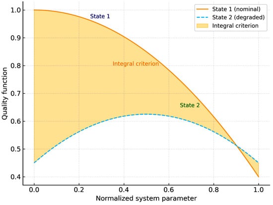
Figure 2. Quality function of the control system in two states and the integral criterion.

Using the obtained results, the performance quality criterion can be determined. The integral performance criterion of the system is defined as the area S_i, which is bounded by the curve $d_{\ast }\left(p\right)$ and the straight line ${\mathrm{d}}_{\ast }=\mathrm{\delta }{\mathrm{d}}_{\ast }$:

$${\mathrm{S}}_{\mathrm{i}}={\displaystyle \underset{{\mathrm{p}}_{\ast \mathrm{j}}^{\prime }}{\overset{{\mathrm{p}}_{\ast \mathrm{j}}^{"}}{\int }}\left({\mathrm{d}}_{\ast \mathrm{i}}\left({\mathrm{p}}_{\ast \mathrm{j}}\right)\right)\mathrm{d}\mathrm{p}}-{\displaystyle \underset{{\mathrm{p}}_{\ast \mathrm{j}}^{\prime }}{\overset{{\mathrm{p}}_{\ast \mathrm{j}}^{″}}{\int }}\left(\mathrm{\delta }{\mathrm{d}}_{\ast }\right)\mathrm{d}\mathrm{p}}.$$

The value of $\mathrm{\delta }{\mathrm{d}}_{\ast }$ corresponds to the boundary of the control system performance, beyond which the system is either incapable of performing its functions or executes them with an accuracy that does not satisfy the requirements for achieving the desired output effect.

The larger the value of the quality criterion, the higher the functional readiness of the system. Moreover, by analyzing the values of S_i amid variations in the independent dual variables (i.e., the probabilities of the system being in operational states), one can derive conclusions regarding the strategy of further system development or the prospects for designing new systems [9,10,11,12,13,14,16].

Figure 3 presents the architecture of the diagnostic–performance module integrated into the automated control system (ACS). The primary source of information is the telemetry database, which accumulates parameters from energy infrastructure objects [16]. These data are transmitted to the KMC/similarity engine, which implements continuous-time Markov chains (CTMC) for modeling system states and assessing their similarity [17,18].

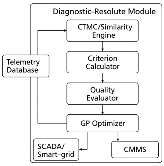
Figure 3. Architecture of the diagnostic–performance module of the automated control system.

The computational cost of the proposed diagnostic module is primarily determined by the evaluation of the matrix polynomial f(Q). Updating the generator matrix requires O(m²), while polynomial evaluation based on (5)–(7) has complexity O(k m³), where k is the small, fixed degree of interpolation (typically k ≤ 5). The subsequent criterion evaluation (9) and computation of the dual GP function (10) add only O(k m) and O(m log(m)), respectively. Therefore, the overall complexity of one diagnostic cycle is O(m³). Empirical tests (Python/NumPy, Version: NumPy 2.3.0. Released: 7 June 2025, BLAS acceleration) show that full computation requires <1 ms for m = 3–5 and ~5–6 ms for m = 10, which fully satisfies the real-time constraints of ACS/SCADA environments. The architecture in Figure 3 supports asynchronous updates, and the system can run at frequencies up to 1–10 Hz, ensuring efficient integration with Smart Grid operational platforms [9,10,19].

Subsequent processing is carried out in the criterion calculator, which generates normalized reliability and availability indicators. The quality evaluator integrates the results to construct the integral performance criterion of the ACS. Based on this criterion, the GP optimizer (geometric programming method) performs ranking and selection of optimal modernization strategies.

The computation results are transferred to external systems: SCADA/Smart Grid platforms, where real-time control actions are implemented, and the CMMS (Computerized Maintenance Management System), which provides maintenance planning. Such an architecture enables the integration of diagnostic algorithms into the production environment, thereby ensuring automated decision support within complex energy networks [9,10,11,12,13,14].

1.5. Example of Calculation for Abrupt Load Changes in the Power Network

A reproducible case of modeling a non-homogeneous continuous-time Markov process is presented for a power system node, where abrupt load changes (disturbances) cause an increase in transition intensities to degraded and failed states according to the input parameters (Table 1). The effect on availability and the energy not supplied (ENS) is demonstrated.

Table 1. Input parameters.

Parameter	Value
Simulation duration	12 h (time step 1 min)
Nominal node power	10.0 MW
Weight of degraded state w2	0.60
Performance in S1/S2/S3	100%, 80%, 0%
Base transition intensities per minute	λ12 = 0.001, λ13 = 0.0002, λ21 = 0.006, λ23 = 0.0008, λ31 = 0.003
Disturbance thresholds	0.85 and 1.05 of nominal; + multiplier for Δ load ≥ 5% per min

Two periods of abrupt changes are observed: a major disturbance reaching 110% of nominal load (240–300 min) and a smaller disturbance occurring at approximately the eighth hour.

According to Figure 4, the baseline load level remains around 0.60 of the nominal value. The major disturbance in the interval at 240–300 min reaches 1.10 of nominal; the average ramp rate in the segment 240–255 min is ≈2% per minute, i.e., below the threshold of 5% per minute required for the additional “dynamic” risk multiplier. The key contribution to the disturbance arises from exceeding the 1.05 threshold, which triggers an eight-fold increase in transition intensities, whereas the second, smaller disturbance (~0.95) does not activate the upper threshold but slightly increases risks due to operation within the ≥0.85 range.

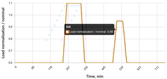
Figure 4. Load profile (fraction of nominal value).

In Figure 5, the multipliers for S₁→S₂ (λ₁₂) and S₂→S₃ (λ₂₃) sharply increase when the load exceeds 105% of the nominal, reaching approximately eight times their base values. In the presented profile, the gradients are smooth (≈2%/min), with the threshold mechanism > 105 > 105% > 105 dominating the risk amplification process.

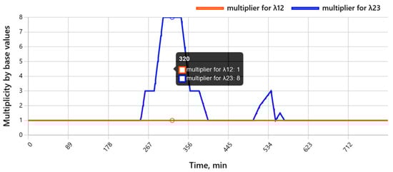
Figure 5. Risk amplification of transitions under disturbances. Multipliers for transition intensities S₁→S₂ (λ₁₂) and S₂→S₃ (λ₂₃).

Figure 6 shows that during the disturbance period, the minimum probability of state P(S₁) ≈ 0.615 (around 04:59), the maximum probability of state P(S₂) ≈ 0.282 (around 04:58), and the probability of state P(S₃) reaches ≈ 0.105\approx 0.105 ≈ 0.105 (around 04:59). This indicates a redistribution of probabilities primarily towards the degraded state, with a moderate but noticeable increase in the failure state.

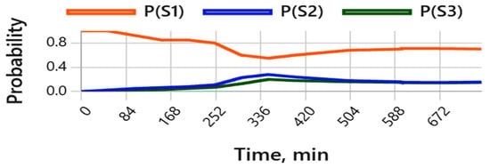
Figure 6. Dynamics of readiness states.

Figure 7 shows that availability A(t) = P(S₁) + w₂P(S₂) drops to a minimum of approximately 0.783 (around 04:59). The average values for the intervals are as follows: before the disturbance A ≈ 0.949, during the disturbance A ≈ 0.856, and after the disturbance A ≈ 0.815. These figures align with the behavior of P(S₁), P(S₂) confirming the sensitivity of the metric to overload modes.

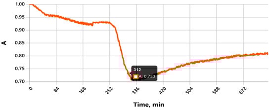
Figure 7. Availability A(t) = P(S₁) + w₂P(S₂). The minimum A coincides with the peaks of the load.

1.6. Energy Loss Calculation

We considered states S₁/S₂/S₃ with productivity of 100%, 80%, and 0%, respectively. Therefore, S(t) = D(t) [1⋅P(S₁) + 0.8⋅P(S₂) + 0⋅P(S₃)], and the difference D(t) − S(t) is integrated over time into the cumulative ENS (Energy Not Supplied) in the graph. This explains why during load disturbances (increased transitions from S₁→S₂, S₂→S₃), ENS increases most rapidly, as shown in Figure 8.

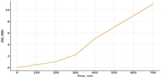
Figure 8. Cumulative ENS (MWh). Growth occurs almost entirely during the main disturbance period.

As seen in Figure 8, the total ENS (over 12 h) is primarily formed during the 240–300 min interval; the ENS during the disturbance accounts for approximately 12.5% of the total. After the overload is removed, the growth of ENS nearly halts, indicating the temporal localization of the losses.

Table 2 and Table 3 show the summary metrics by interval and the estimated event frequency (averaged over runs)

Table 2. Summary metrics by intervals.

Interval	Average A	ENS, MWh	Comment
Before disturbance (0–240 min)	0.948	0.881	System in nominal; losses minimal
During disturbance (240–300 min)	0.842	1.302	Failure of readiness; main contribution to ENS
After disturbance (300–720 min)	0.770	8.946	Recovery with residual effects

Table 3. Estimated event frequency (averaged across runs).

Transition Type	Number over 12 h (Total Across Runs)
S1-S2	351
S1-S3	67
S2-S1	210
S2-S3	75
S3-S1	93

Let us show the sensitivity of the ENS to the amplitude of the disturbance, in Figure 9.

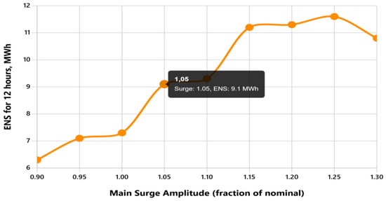
Figure 9. Sensitivity of ENS to disturbance amplitude.

As shown in Figure 9, the dependence of ENS on the disturbance amplitude exhibits a “knee” nearly 1.05× nominal: for 1.00× → ENS ≈ 7.674 MWh; 1.05 → ENS ≈ 10.491 MWh; 1.10 → ENS ≈ 10.445 MWh; and 1.20 → ENS ≈ 10.836 MWh. After exceeding 105%, the curve becomes significantly steeper due to the activation of increased transition intensities.

According to the calculations, abrupt load changes significantly increase the probability of transitions to degraded and failure states, as evidenced by the drop in availability A(t) and the concentration of energy losses (ENS) during the disturbance period. Controlled load reduction and limiting the amplitude to <105% of the nominal significantly reduce ENS. It is recommended to implement policies for pre-emptive load reduction, fast AR (automatic reconnection)/AFC (Automatic Frequency Control) schemes, and prioritization of recovery after periods of high disturbance.

The theoretical derivation of the similarity criteria π_i relies on the steady-state form of the CTMC to define the normalization properties and the structural characteristics of the generator matrix Q. In operational settings, however, the system is non-stationary and λ_ij(t) vary with load. In this case, the model employs a quasi-stationary approach: at each time step the instantaneous generator matrix Q(t) is substituted into the polynomial f(Q), and the normalized criteria π_i(t) and performance indicators are computed for that moment. Since load variations occur on a slower time scale than the analytical cycle, the instantaneous evaluation remains accurate and fully consistent with the mathematical framework established in Section 2.

The quality performance criterion model based on Markov processes has been applied to distributed automated control systems for Smart Grid, where quality is presented as a Markov reward J = π·r, with π being the stationary (or quasi-stationary) state distribution, and r being the weight/utilization vector. The practical readiness indicator, A(t)= P(S₁,t) + w₂·P(S₂,t), is consistent with SLO/SLA.

The non-homogeneity of the modes is reflected in the time-dependent intensities λ_ij(t), which increase upon exceeding the power threshold (~105% of nominal) and high rates of change (≥5%/min). This raises the probabilities of transitions S₁→S₂ and S₂→S₃. The model parameters are identified from operational logs (MLE: $\hat{\mathrm{\lambda }}$_ij = N_ij/T_i) with the construction of confidence intervals and regular re-estimation in sliding windows, suitable for online monitoring. Uncertainty and confidence are assessed through posterior simulations (gamma models), providing intervals for A and derivative metrics, thus enhancing the reliability of management decisions (maintenance, switching, and load limitation) [20].

The data pipeline “OPC UA/REST → TimescaleDB/PostgreSQL → analytical service” supports real-time operation with end-to-end latency of 20–40 ms, while the analytical cycle (CTMC update, similarity indices, criterion computation, GP optimization) requires 1–6 ms, well within the typical SCADA/Smart Grid limits of 100–200 ms. Transition intensities λ_ij are re-estimated from operational logs using a sliding time window, whose size depends on the dynamism of the node: 5–15 min (updated every 1–5 min) for nominal conditions and 1–3 min (updated every 20–60 s) during dynamic disturbances or overloads. This ensures statistically stable MLE estimates while maintaining rapid adaptation. The selected window sizes guarantee sufficient event counts for reliable estimation (≥30–50 nominal/degraded transitions, ≥5–10 failure transitions) and provides a practical guideline for real-world Smart Grid implementations.

Sensitivity analysis shows that the greatest impact on readiness during disturbances is exerted by λ₁₂ and λ₂₃ (degradation → failure); these should be limited by controlled load strategies and accelerated recovery.

Therefore, engineering actions should focus on minimizing ENS and stabilizing A(t), limiting disturbance amplitude to <105% of nominal, limiting the gradients of power change, applying preventive isolation/redistribution, and prioritizing recovery from S₂ to S₁.

The model is actively integrated into the ACS/SCADA system. It is embedded into OPC UA/REST → TimescaleDB/PostgreSQL → analytical service (π, A, ENS) → Grafana/SCADA-HMI, ensuring continuous quality assessment and automated threshold triggers. Moreover, this approach can be extended to multi-component nodes, it supports weights for degradation classes, and it has been expanded to semi-Markov models for long-tail durations.

When transition intensities depend on load, the generator matrix becomes time dependent, Q(t). The similarity criteria are then evaluated using a quasi-stationary approximation, where the instantaneous matrix Q(t) is substituted into the polynomial representation f(Q(t)) = ∑a_jQ(t)^j, yielding time-dependent normalized criteria π_i(t). This approximation is valid when the analytical cycle Δt is much smaller than the characteristic time of load variation. In Smart Grid applications Δt = 1–6 ms, while load dynamics occur over seconds to minutes, ensuring the time scale separation:

‖Q′(t)‖Δt ≪ ‖Q(t)‖.

Thus, the steady-state theoretical constructs serve as normalization and structural foundations, while real-time operation is handled through a sequence of instantaneous evaluations of Q(t), enabling accurate diagnostics during dynamic disturbances.

Thus, the Markov process-based quality performance criterion model is a practically applicable tool for operational management and strategic planning: it transforms failure/recovery dynamics into transparent metrics (readiness, ENS) and provides verified foundations for decision making in load disturbance modes.

1.7. Comparison of Different Stochastic Modeling Approaches

Table 4 presents a systematic comparison of the key stochastic modeling approaches. For each model, the main assumptions, advantages, and limitations, as well as typical software tools and areas of practical application, are outlined. This provides a well-grounded basis for selecting an appropriate mathematical framework for assessing the reliability, controllability, and efficiency of automated control systems (ACS).

Table 4. Comparative characteristics of different stochastic modeling approaches.

Model	Key Assumptions	Advantages	Limitations	Typical Tools	Applications
CTMC (Continuous-Time Markov Chains)	Memoryless (Markov property); stationary transition rates	Analytical tractability, compactness (Q-matrix), and suitable for failure/repair analysis	Does not capture history dependence; difficult with large state spaces	SHARPE, Matlab, (version R2023b) and Python (NumPy/SciPy)	Reliability/availability; Smart Grid ACS
SMP (Semi-Markov Processes)	Non-stationary/arbitrary state holding time distributions	More realistic durations; generalization of CTMC	Complex estimation/identification of distributions; harder analytics	SHARPE; custom implementations	Maintenance with non-uniform service times
MDP (Markov Decision Processes)	Markovian transitions with control actions	Policy optimization; integration with reinforcement learning	High dimensionality; requires precise reward model	MDPtoolbox; RL libraries	Optimization of maintenance/switching strategies
Petri Nets/SRN	Stochastic events/places/transitions	Expressiveness for concurrency	Calibration complexity; computational cost	GreatSPN; TimeNet	Complex distributed architectures
RBD/FTA (Reliability Block Diagrams/Fault Tree Analysis)	Block structure; independent failures	Simplicity, visualization	Weak dynamics; limited for repair/queuing	ReliaSoft; BlockSim	High-level system design
Bayesian Networks	Probabilistic dependencies among components	Learning from data; handling uncertainty	Requires data or expert priors; structural complexity	GeNIe/SMILE; pgmpy	Diagnostic and causal analysis

The conducted study has demonstrated that the proposed approach, based on the integration of Markov modeling with the framework of geometric programming, provides higher accuracy in evaluating the functional readiness of ACS compared to classical stochastic and structural models. Unlike CTMC, RBD/FTA, or Petri nets, which are limited by simplifying assumptions or substantial computational costs, the developed method enables the derivation of normalized similarity criteria and an integral performance indicator that encompasses all possible system states. This makes it possible to generate quantitatively justified evaluations of operability even under conditions involving multistate behavior, probabilistic failures, and partial data uncertainty.

2. Conclusions

This study developed and validated a criterion-based model for evaluating the functional readiness of distributed automated control systems (ACS) using continuous-time Markov processes and geometric programming. The results demonstrate that the proposed approach enables a comprehensive and quantitatively consistent assessment of system performance across all operational states, including nominal, degraded, and failure modes. The constructed matrix polynomial and normalized similarity indices π_i form a unified integral quality indicator that does not require global optimization and remains computationally efficient.

The numerical experiments revealed that ACS readiness is highly sensitive to overload conditions: when the load exceeded 105% of nominal, the transition intensities to degraded and failure states increased by nearly an order of magnitude, causing availability to drop to 0.783 and significantly accelerating system degradation. The modeling also showed that the majority of energy not supplied losses (ENS) accumulated during short periods of dynamic disturbances, particularly in the interval between 240 and 300 min, which accounted for more than 12.5% of total ENS over the 12 h simulation. A pronounced “knee point” was observed near the 105% load threshold, where ENS begins to rise sharply, highlighting the practical value of maintaining load levels below this boundary.

In terms of computational performance, the proposed analytical cycle—including CTMC updates, similarity calculations, criterion evaluation, and geometric programming optimization—requires only 1–6 ms, making the method suitable for real-time operation within SCADA and Smart Grid environments. The model also proved effective for comparing modernization scenarios, assessing parameter sensitivities, and supporting operational and strategic decision making in distributed ACS. The obtained results confirm that preventive load-management strategies, especially limiting peak loads below 105% of the nominal, substantially improve system readiness and reduce ENS, demonstrating the practical applicability of the developed criterion model for modern power systems.

References

- Heimann, D.I.; Mittal, N.T.K.S. Availability reliability modeling for computer systems. In Advances in Computers; Marshall, C.Y., Ed.; Academic Press: San Diego, CA, USA, 1990; Volume 31, pp. 175–233. [Google Scholar]
- Muppala, J.K.; Malhotra, M.; Trivedi, K.S. Markov dependability models of complex systems: Analysis techniques. In Reliability and Maintenance of Complex Systems; Slileyman, O., Ed.; Springer: Berlim, Germany, 1996; pp. 442–486. [Google Scholar]
- Hisashi, M.; Shunji, O. Markovian Decision Processes; Elsevier Pub. Co.: Amsterdam, The Netherlands, 1970; 142p. [Google Scholar]
- Sahner, R.; Trivedi, K.S.; Puliafito, A. Performance and Reliability Analysis of Computer Systems: An Example-Based Approach Using the SHARPE Software Package; Kluwer Academic Publishers: Dordrecht, The Netherlands, 1996; 404p. [Google Scholar]
- Yukhimchuk, M.; Kovtun, V.; Horchuk, Y.; Lesko, V. Algorithmic methods of constructing the space of parameter increments in automated control systems of energy processes. In Proceedings of the MoMLeT-2025: 7th International Workshop on Modern Machine Learning Technologies, Lviv-Shatsk, Ukraine, 14 June 2025. [Google Scholar]
- Yukhymchuk, M.; Dubovoi, V.; Kovtun, V. Decentralized Coordination of Temperature Control in Multiarea Premises. Complexity 2022, 2022, 18. [Google Scholar] [CrossRef]
- Yukhymchuk, M.; Dubovoi, V.; Kovtun, V. Grochla Functional Dependability of Distributed Control of Multi-zone Objects under Failures Conditions. IEEE Access 2024, 12, 95736–95749. [Google Scholar]
- Zhang, Y.; Wang, L.; Sun, H. Data-driven reliability assessment of smart grids: A survey. Renew. Sustain. Energy Rev. 2020, 120, 109632. [Google Scholar]
- Ghosh, S.; Chatterjee, S. A review on reliability, resilience, and cyber security of the smart grid. Electr. Power Syst. Res. 2020, 189, 106602. [Google Scholar]
- Lin, Y.; Wen, J.; Wu, Q. Reliability assessment of distribution networks with renewable energy based on continuous-time Markov chains. Appl. Energy 2019, 253, 113598. [Google Scholar]
- Huang, Y.; Xu, Y.; Liu, H.; Wang, Z. A Markov decision process-based approach for energy management in smart grids. Appl. Energy 2020, 269, 115085. [Google Scholar]
- Zhou, K.; Fu, C.; Yang, S. Big data driven smart energy management: From big data to big insights. Renew. Sustain. Energy Rev. 2019, 79, 1099–1118. [Google Scholar] [CrossRef]
- He, X.; Fang, X.; Wang, J.; Dong, Z.Y. Smart grid resilience: A review. IEEE Trans. Smart Grid 2019, 10, 5702–5716. [Google Scholar]
- Li, W.; Wang, B.; Zhao, D.; Zhou, Y.; Guo, C. Hybrid modeling and reliability assessment for cyber–physical smart grids. Energy Rep. 2021, 7, 6147–6156. [Google Scholar]
- Cheng, L.; Wei, X.; Li, M.; Tan, C.; Yin, M.; Shen, T.; Zou, T. Integrating Evolutionary Game-Theoretical Methods and Deep Reinforcement Learning for Adaptive Strategy Optimization in User-Side Electricity Markets: A Comprehensive Review. Mathematics 2024, 12, 3241. [Google Scholar] [CrossRef]
- Mahmood, F.; Javaid, N.; Rahim, M.H.; Imran, M.; Guizani, M. Smart grid communication and information technologies in the perspective of Industry 4.0: Opportunities and challenges. Comput. Netw. 2020, 171, 107–118. [Google Scholar]
- Bisikalo, O.; Kharchenko, V.; Kovtun, V.; Krak, I.; Pavlov, S. Parameterization of the Stochastic Model for Evaluating Variable Small Data in the Shannon Entropy Basis. Entropy 2023, 25, 184. [Google Scholar] [CrossRef] [PubMed]
- Ramadan, I.S.; Harb, H.M.; Mousa, H.M.; Malhat, M.G. Reliability Assessment for Open-Source Software Using Deterministic and Probabilistic Models. Int. J. Inf. Technol. Comput. Sci. 2022, 14, 1–15. [Google Scholar] [CrossRef]
- Aminifar, F.; Fotuhi-Firuzabad, M.; Shahidehpour, M.; Khodaei, A. Cyber resilience framework for smart grids: A review. IEEE Trans. Smart Grid 2020, 11, 4820–4830. [Google Scholar]
- Xu, Y.; Li, K.; Zeng, P.; Xu, W. Reliability evaluation of cyber–physical power systems considering cyber-attacks. Int. J. Electr. Power Energy Syst. 2019, 110, 634–641. [Google Scholar]
Disclaimer/Publisher’s Note: The statements, opinions and data contained in all publications are solely those of the individual author(s) and contributor(s) and not of MDPI and/or the editor(s). MDPI and/or the editor(s) disclaim responsibility for any injury to people or property resulting from any ideas, methods, instructions or products referred to in the content. |
© 2025 by the authors. Licensee MDPI, Basel, Switzerland. This article is an open access article distributed under the terms and conditions of the Creative Commons Attribution (CC BY) license (https://creativecommons.org/licenses/by/4.0/).