Featured Application
The XY → code and code → extent algorithms operate in constant time O(1), simplifying the organization and access to nationwide remote sensing data and reducing reliance on costly topological operations. The hierarchical PL-2000 structure supports multi-scale aggregation and decomposition without changing data structures, and unified boundary rules ensure deterministic behavior at boundaries and stable resolution switching. Replacing regular string-based map sheet code scheme with a single 32-bit Long key simplifies indexing and allows for a 3–8× reduction in the code file size and a noticeable speedup in filters and joins in database systems. The approach is transferable to other national coordinate reference systems, where map-sheet identification schemes can be transformed into high-performance indices for modern remote sensing and GeoAI.
Abstract
Efficient spatial indexing is critical for processing large-scale remote sensing datasets (e.g., LiDAR point clouds, orthophotos, hyperspectral imagery). We present a bidirectional, hierarchical index based on the Polish PL-2000 coordinate reference system for (1) direct computation of a map-sheet identifier from metric coordinates (forward encoder) and (2) reconstruction of the sheet extent from the identifier alone (inverse decoder). By replacing geometric point-in-polygon tests with closed-form arithmetic, the method achieves constant-time assignment O(1), eliminates boundary-geometry loading, and enables multi-scale aggregation via simple code truncation. Unlike global spatial indices (e.g., H3, S2), a CRS-native, aligned with cartographic map sheets in PL-2000 implementation, removes reprojection overhead and preserves the legal sheet semantics, enabling the direct use of deterministic O(1) numeric keys for remote-sensing data and Polish archives. We detail the algorithms, formalize their complexity and boundary rules across all PL-2000 zones, and analyze memory trade-offs, including a compact 26-bit packing of numeric keys for nationwide single-table indexing. We also discuss integration patterns with the OGC Tile Matrix Set (TMS), ETL pipelines, and GeoAI workflows, showing how bidirectional indexing accelerates ingest, training and inference, and national-scale visualization. Although demonstrated for PL-2000, the approach is transferable to other national coordinate reference systems, illustrating how statutory map-sheet identification schemes can be transformed into high-performance indices for modern remote sensing and AI data pipelines.
1. Introduction
Efficient spatial indexing is critical for processing large-scale remote sensing datasets, including LiDAR point clouds, orthophotos, hyperspectral imagery, and elevation models [1,2,3]. In geographic information systems, the planar point location problem—uniquely determining an object’s position within a reference grid—remains fundamental both for classical cartographic applications and for modern datasets driven by artificial intelligence and geospatial artificial intelligence (GeoAI) [4]. In operational practice, deterministic, constant-time assignment of samples to spatial partitions (tiles or map-sheets) reduces I/O (input/output), simplifies ETL (Extract, Transform, Load) stages, supports multi-scale analyses, and increases throughput across the entire pipeline—from acquisition to training, inference, and national-scale visualization [5].
Global hierarchical partitioning paradigms—Discrete Global Grid Systems (DGGS), Google’s S2, Uber’s H3, Geohash, Quadbin—provide geometric consistency and planet-wide scalability [6,7,8,9]. However, their direct use within national coordinate reference systems (e.g., PL-2000) requires reprojection and is often difficult to reconcile with statutory cartographic standards and administrative practice, undermining alignment with the legally defined map-sheet hierarchy [10]. DGGS is global, hierarchical, and supports multiple spatial resolutions. It divides the Earth into “a hierarchy of equal area tessellations to partition the surface of the Earth into cells” of unique IDs [11,12]. DGGS cells can be of different shapes, e.g., squares, triangles or hexagons—the last ones being a viable alternative to most common square grids [13]. Two open-source DGGS implementations were analyzed during algorithmic testing: Uber’s H3 and Google’s S2. Uber’s H3 uses a hexagonal grid to index points and polygons, with 15 available resolutions. The resulting index is a sequence of hierarchical digits, each from 0 to 6 (stored as uint64) [10]. Google’s S2 works exclusively for spherical projections. Each cell is a quadrilateral, subdividing into another 4 cells in 31 specified levels [9]. Other hierarchical spatial indexing systems are, e.g., Geohash, which allows for rectangular divisions of the entire globe with 12 precision levels [14], which was also analyzed in this paper, HEALPix using diamond-shaped cells, which is useful, e.g., in astronomy [15], and many other implementations.
In parallel, web tiling standards such as the OGC Tile Matrix Set (TMS) offer a practical multi-scale partitioning model for services and caches [16]. Classical spatial indexes (R-tree, quadtree) remain widely used but generally incur logarithmic query costs, depend on explicit boundary geometries, and are not aligned with the semantics of national map-sheets—limitations that matter when massively assigning records to a fixed grid. R-trees are hierarchical spatial indexes introduced in 1984, and still widely used. The geometry is organized with the use of tree of bounding boxes (minimum bounding rectangles (MBRs) [17]. Quadtrees also operate in a tree structure—each node has exactly four children—equal-area quadrants. Due to their simplicity, they are widely used in raster data operations, e.g., tiling and building image pyramids [18,19].
Despite the diversity of the existing algorithms, none of them provide a constant-time (O(1)) encoder/decoder aligned with a national map-sheet hierarchy together with a simple, numeric index, based solely on map sheet sections in particular scales. Divisions used by the existing approaches do not align with cartographic sheet boundaries within local CRS—reprojections are required. As a result, the literature lacks a formally specified, closed-form, easy-to-implement O(1) indexing method that operates directly within PL-2000 or comparable national projection systems.
We propose a bidirectional, hierarchical indexing method native to PL-2000 that:
- Computes the map-sheet code (XY → code) in O(1) using closed-form integer arithmetic;
- Reconstructs the sheet extent (code → extent) from the identifier alone, without loading boundary geometries;
- Supports multi-scale aggregation/decomposition via simple truncation/extension of the code suffix;
- Provides a compact numeric representation (e.g., 26-bit packing) that reduces memory costs and accelerates joins and filtering;
- Integrates with TMS/ETL/GeoAI pipelines, accelerating ingest, training and inference, and visualization at national scale.
The algorithm was primarily designed to provide an efficient solution for spatial data indexing stored in archives, particularly in national planar coordinate systems to avoid transformations, and enable quick search and performing spatial queries. This paper fills this gap for PL-2000, but with possible implementations in other CRSs, by:
- Using closed-form arithmetic algorithms for determining XY → sheet-code and code → extent (Section 2);
- Specifying deterministic boundary rules valid across all PL-2000 zones (Section 2);
- Providing a short uint32 index (including 26-bit packing) that is possible to integrates with modern RS/OGC/GeoAI workflows.
This work relates particularly to the author’s earlier studies on sheet systems (including in the context of the International Map of the World) [20,21], but the formulas, boundary-case rules, and validation protocol presented here are developed specifically for PL-2000, ensuring novelty relative to prior implementations. The remainder of this paper is organized as follows: Section 2 presents the materials and methods (PL-2000 background, algorithms, numeric representation); Section 3 reports the results; Section 4 provides a discussion; and Section 5 presents the conclusions.
2. Materials and Methods
2.1. The PL-2000 Coordinate System
2.1.1. Definitions and Projection Parameters (ETRS89/GRS80, Zones 5–8)
The PL-2000 coordinate system (ETRF2000-PL/CS2000) is one of the official national map projections used in cartographic and geodetic production, particularly for large-scale maps and models. Based on the ETRS89 reference frame and the GRS80 ellipsoid, it defines plane rectangular coordinates in meters, with axes X—northing—and Y—easting. The system divides Poland into four projection zones with central meridians at 15° E, 18° E, 21° E, and 24° E, labeled 5, 6, 7, and 8. Each zone is 3° of longitude wide, which limits projection distortions and provides a natural first level of data indexing (Figure 1). Easting values include an offset (false easting value) of 5,500,000, 6,500,000, 7,500,000 or 8,500,000, depending on the zone. Each zone has its own definition, along with the EPSG codes: 2176-2179.
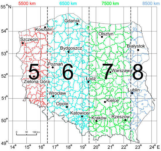
Figure 1.
Division of Poland into four three-degree Gauss–Krüger projection zones—central meridians 15° E (zone 5), 18° E (zone 6), 21° E (zone 7), 24° E (zone 8).
In remote sensing practice, this subdivision enables rapid restriction of the search space (distributed ETL, tiling, caching). At the level of numeric storage, the zone digit (5–8) appears as the “million prefix” of the Y component, which allows for unambiguous zone recognition using integer arithmetic without additional geometric tests [22,23].
2.1.2. Sheet System and Code Grammar (1:10,000 → 1:500)
The base unit is a 1:10,000 sheet measuring 5 km (N–S) × 8 km (E–W). The structure is hierarchical: a 1:10,000 sheet subdivides either into four sheets (2 × 2, the 1:5000 variant) or into twenty-five sheets (5 × 5, the 1:2000 variant) (Figure 2). A 1:2000 sheet is then split into four sheets (2 × 2) to reach 1:1000, and again into four sheets (2 × 2) to reach 1:500 (Figure 3). In consequence, the map-sheet identifier (sheet code) acts as a deterministic key that uniquely specifies location and scale level—particularly useful in RS big-data streams (LiDAR, orthophoto, HSI) and GeoAI pipelines.
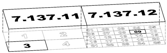
Figure 2.
Example subdivision of sheet 7.137.11 (1:10,000) into four 1:5000 sheets and of sheet 7.137.12 (1:10,000) into twenty-five 1:2000 sheets.
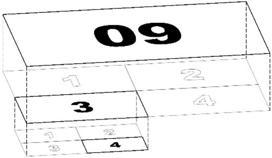
Figure 3.
Subdivision of sheet 7.137.12.09 (1:2000) into four 1:1000 sheets, and then into four 1:500 sheets; example final 1:500 sheet code: 7.137.12.09.3.4.
The hierarchical sheet system in PL-2000 supports strict multi-resolution partitioning, in which spatial datasets of different scales are assigned to sheet levels that preserve positional consistency across resolutions. This is ensured by deterministic parent–child relations defined by the 2 × 2 and 5 × 5 subdivisions. A key advantage is the ability to assign each data sample to its sheet by computing the sheet code, eliminating costly spatial operations and supporting efficient processing in big-data and AI workflows.
We explain the hierarchical system based on a sheet code at 1:10,000. It comprises three numbers, presented as A, BBB and CC, where:
- A is a single digit denoting the projection zone (central meridian) 5, 6, 7, or 8, defined by: A = L0/3,where L0 is the central meridian of the zone (15°, 18°, 21°, or 24°).
- BBB is a three-digit integer:BBB = int((x1 − 4920)/5)where x1 is the X coordinate (northing) of any point within the 1:10,000 sheet’s area, expressed in kilometers from the equator.
- CC is a two-digit integer:CC = int((y1 − 332)/8)where y1 is the Y coordinate (easting) of any point within the 1:10,000 sheet’s area, expressed in kilometers with the leading zone digit removed (i.e., without the initial 5/6/7/8).
The 1:10,000 code A.BBB.CC is extended by suffixes determined by the subdivision level:
- 1:5000: 2 × 2 split, s ∈ {1, 2, 3, 4};
- 1:2000: 5 × 5 split, SS ∈ {01 … 25};
- 1:1000: another 2 × 2, s1k ∈ {1, 2, 3, 4};
- 1:500: another 2 × 2, s500 ∈ {1, 2, 3, 4}.
Hence, the full code at 1:500 is organized as follows: A.BBB.CC[.SS][.s1ₖ][.s500], where each additional token unambiguously indicates a finer scale and the position in the hierarchy (Table 1).

Table 1.
Hierarchical subdivision of a 1:10,000 sheet in the PL-2000 system.
2.2. Algorithm for Computing the Sheet Code (XY → Code)
2.2.1. Assumptions, Notation, Complexity
Goal: for a point (X, Y) in the PL-2000 system, compute the hierarchical map-sheet code at a target scale ∈ {1:10,000, 1:5000, 1:2000, 1:1000, 1:500}. Axis convention (official in PL-2000): X—northing (m), Y—easting (m).
The base 1:10,000 sheet measures 5 km (N–S) × 8 km (E–W) and has code A.BBB.CC, where A∈{5..8} is the zone number (the million digit in Y), BBB is the row (every 5 km counted from 4920 km), and CC is the column (every 8 km counted from 332 km after trimming the million). Finer scales add suffixes as follows: 1:5000—2 × 2; 1:2000—5 × 5 (01..25); 1:1000—2 × 2; 1:500—2 × 2.
For edge stability, use a perturbation ε ≈ 1 × 10⁻⁸ m added to X and Y. Time and memory complexity: O(1)—arithmetic only, no geometry.
2.2.2. Method (Step-by-Step)
- (Optional) Check the PL-2000 domain: zones A ∈ {5..8} and the working ranges of X,Y.
- Apply edge perturbation: X ← X + ε; Y ← Y + ε.
- Compute the 1:10,000 base part:
- A = floor(Y/106);
- BBB = floor((X/1000 − 4920)/5);
- CC = floor(((Y mod 106)/1000 − 332)/8)
- code = A.BBB.CC (with CC formatted as two digits).
- if targetScale = 1:5000—append the 2 × 2 index (s ∈ {1..4}), or
- if targetScale ≤ 1:2000—append the 5 × 5 index (SS ∈ {01..25}),if targetScale ≤ 1:1000—append 2 × 2 index (s ∈{ 1..4}),if targetScale = 1:500—append 2 × 2 index (s∈ {1..4});
- Return the hierarchical code, e.g., 6.122.15.03.2.1.
The pseudocode for the above method (VB6-friendly) is included in the Supplementary Materials.
2.3. Algorithm for Reconstructing the Sheet Extent (Code → Min–Max)
2.3.1. Assumptions, Notation, Complexity
Input: hierarchical sheet code A.BBB.CC[.SS][.s][.s], where A∈{5..8}; BBB—row at 1:10,000 (every 5 km); CC—column at 1:10,000 (every 8 km); SS∈{01..25}—the 5 × 5 subdivision, (1:2000); s ∈ {1..4}—2 × 2 subdivisions (for 1:5000, 1:1000, 1:500).
Output: bounding rectangle Pmin = (Xmin, Ymin), Pmax = (Xmax, Ymax).
Convention: X—northing (m), Y—easting (m).
Complexity: O(1); no boundary geometry I/O.
2.3.2. Method (Step-by-Step)
- Parse the code: remove dots and convert to digits G(1..n); infer the scale from length n: 6 → 1:10,000, 7 → 1:5000, 8 → 1:2000, 9 → 1:1000, 10→1:500.
- From A,BBB,CC compute the upper-left corner of the 1:10,000 sheet (in meters):X_top = (BBB·5 + 4925)·1000; Y_left = (CC·8 + 332)·1000 + A·1 000 000.
- If scale = 1:5000—apply the 2 × 2 subdivision (index s) to update Y_left/X_top.
- If scale ≤ 1:2000—apply 5 × 5:X_top ← X_top − ⌊(SS − 1)/5⌋·1000; Y_left ← Y_left + ((SS − 1) mod 5)·1600;If scale ≤ 1:1000—apply 2 × 2 (S = 1000); if scale = 1:500—apply an additional 2 × 2 (S = 500).
- Return: Pmin = (X_top − scale·0.5, Y_left), Pmax = (X_top, Y_left + scale·0.8).
Practical remark: the offsets used in the Return function are equal to scale·0.5 for X, and scale·0.8 for Y as they directly correspond to the sheet dimensions in particular scales. For example, 1:500 sheets are 250 (500·0.5) m × 400 (800·0.5), and 1:10,000 sheets are 5000 m × 8000 m.
The pseudocode for the above method (VB6-friendly) is included in the Supplementary Materials.
2.4. Code Representation (STRING vs. Long) and a Bit-Packed Variant
2.4.1. Rationale and Memory Footprint
A string-based sheet code (e.g., 6.122.15.03.2.1) is human-readable but inefficient for filtering/joins and consumes more memory than an integer. Replacing it with a single 32-bit Long key simplifies indexing and typically speeds up ETL/SQL operations.
How much memory does a STRING sheet code use (character payload only; header overhead ignored)?
- 1:10,000 → A.BBB.CC → 8 characters → ~16 B (VB6/VBA: 2 B/char);
- 1:5000 → A.BBB.CC.s → 10 characters → ~20 B;
- 1:2000 → A.BBB.CC.SS → 11 characters → ~22 B;
- 1:1000 → A.BBB.CC.SS.s → 13 characters → ~26 B;
- 1:500 → A.BBB.CC.SS.s.s → 15 characters → ~30 B.
Note: In VB6/VBA, strings are Unicode (BSTR); so, there is additional per-string overhead (length + terminator), typically ~6–10 B.
For comparison: Long = 4 B.
Savings: at 1:500, moving from ~30 B (plus overhead) to 4 B yields roughly 7–8× less data per record (excluding DBMS metadata).
For memory overhead, storing the code as a STRING consumes approximately ~16 B (1:10,000) to ~30 B (1:500) per record (allocator overhead not included), whereas the Long key is 4 B. In practice, this yields a 3–8× reduction in the code file size and a noticeable speedup in filters and joins in database systems. The summary of approximate memory per code representation can be seen in Table 2.
Table 2.
Approximate memory per code representation.
2.4.2. A Simple Numeric Key (Long) Instead of STRING
If each PL-2000 zone (5–8) is stored in its own repository/table, the zone number does not need to be included in the key itself. The key is built layer by layer, mirroring the sheet hierarchy:
- Start with 1:10,000.Start from the base address of the 10k sheet: the row/column pair. This forms the core of the key.
- Step to 1:2000.The 10k sheet is subdivided into a 5 × 5 grid. Append the small-cell index (01..25) to the core. Conceptually, you are adding one “digit” in base 25.
- Step to 1:1000 and 1:500.Each subsequent level (1:1000, then 1:500) is a 2 × 2 split. Each time, append the quadrant (1..4). Conceptually, you are adding a “digit” in base 4.
The result is a single Long integer that encodes the path:
(10k core) → (5 × 5 cell for 2k) → (quadrant for 1k) → (quadrant for 500).
Decoding works in reverse by “peeling off” layers from the end. First read the last quadrant (1:500), then the previous one (1:1000), next the 5 × 5 cell (1:2000), and finally the 10k row/column core. In practice this is a simple “take the last symbol, remove it, take the previous…” routine.
Aggregation to coarser scales (e.g., from 1:500 to 1:1000 or 1:10,000) is just truncating one or two trailing symbols, with no need to reconstruct coordinates.
Why is this convenient?
- A single type (Long) instead of a text string;
- Fast sorting and joins (the key preserves spatial order within a 10k sheet);
- Easy scale transitions by appending/truncating trailing “symbols”;
- No room for typographic errors typical of STRING representations.
2.4.3. Implementation Guidelines
While using C programming language, to have a single country-wide key and to keep values strictly non-negative:
- Use an explicit, safe unsigned type: uint32_t (4 B, always non-negative).
- Map zones 5, 6, 7, 8 → 1, 2, 3, 4 (the leading “zone” digit): zone4 = A − 4 → zone4 ∈ {1, 2, 3, 4}.
- Maintaining separate repositories per zone allows for sticking to a simple Long (without the zone embedded), which is the simplest and lightest option.
In Visual Basic 6.0, use bit packing when a single table covers all zones and/or scale aggregation is carried out via masking. Use a lightweight bit layout (e.g., 26–28 bits) in which the component fields (BBB, CC, SS, the 2 × 2 quadrants) plus 2 bits for the zone fit into a Long. This way supports nationwide uniqueness, and up-scaling operations reduce to simple bit masks or integer division.
Specific implementation guidelines can be summarized as follows:
- VB6/VBA: store the key as Long (4 B).
- VBA/VB6 in Bentley MicroStation: the built-in Point3d type is used; in systems without this structure, use a neutral equivalent (e.g., your own Point3D record with X, Y, Z) or three numeric columns.
- C/C++: prefer uint32_t (4 B) for portability; if merging zones, add zone4 ∈ {1..4} as the most significant digits (positional system).
- DBMS: index on the numeric key; this typically accelerates joins and range filters vs. VARCHAR.
- Reporting: the textual sheet code can be reconstructed from the numeric key when needed.
2.5. Integration with RS/OGC/GeoAI Pipelines (ETL, Tiles/TMS, Training/Inference)
The bidirectional indexing proposed here (XY → code and code → min–max) turns the sheet code into a universal identifier of a spatial fragment, not merely a cartographic label. As such, it can serve as the backbone that organizes the flow of remote sensing data—from acquisition and preprocessing, through publishing via tiled services, to training and inference in GeoAI systems. The key advantages are constant-time O(1) operation, no need to load boundary geometries, and hierarchy, which enables straightforward switching between operational scales [24].
2.5.1. Data Ingest and Organization (ETL)
In a classical ETL pipeline, the sheet code enables deterministic assignment of records (points, pixels, objects) to the correct spatial units. Instead of costly point-in-polygon tests, closed-form arithmetic is used: each record can be assigned a sheet code at the target scale and then used for ordering and aggregation. This facilitates:
- Building consistent per-sheet partitions in data stores;
- Creating quality metrics and statistics (counts, density, gaps) for specific sheets;
- Simple multi-source consolidation—the sheet acts as a common join key across rasters, vectors, and point clouds.
Consequently, the data-organization stage becomes independent of external spatial services; sorting, filtering, and joins operate on numeric fields (the textual code or the Long key), which typically accelerates ETL and simplifies maintenance.
2.5.2. Publishing and Tiling (OGC Tiles/TMS)
The hierarchical nature of the code aligns well with tiling. Two scenarios are common:
- Native PL-2000 pyramid: tile = sheet at a given scale. The code serves as the tile name or key, and the code → min–max mapping provides the rendering envelope. This preserves the semantics of national map-sheets, important in administration and engineering.
- Publishing in an existing TMS (e.g., Web Mercator): sheets are stored and versioned “our way,” while the service receives imagery rendered on the fly. The decision of which sheets to draw for a given view is made arithmetically, based on their min–max extents.
In both variants, stable naming (code/key) supports effective caching and straightforward resource versioning.
2.5.3. GeoAI: From Sampling to Inference
The sheet code functions as a stable spatial address. It enables easy random/stratified sampling and splitting into training/validation/test sets—without maintaining complex file lists. The same code guarantees reproducible splits.
Furthermore, each code uniquely defines the sheet’s bounding rectangle. Input tiles can be cropped directly to the required footprint, with an optional context buffer—no additional geometry or GIS services required.
Considering inference (online), it is best to convert XY coordinates to a sheet code instantly and route the data chunk to the appropriate model/service (e.g., per sheet or region). Multi-scale aggregation is just changing the code level; so, the processing resolution can be adjusted without recomputing geometries.
2.5.4. Consistency, Versioning, and Audit
Sheet codes promote reproducibility: analytical and training outputs can be linked to specific sheet identifiers and their state (version). A minimal metadata set (scale, code/key, min–max extent, record count, checksum) suffices to reconstruct an experiment or tile publication. Because the index operates in O(1), edge tests (especially near sheet and zone boundaries) can be performed systematically and inexpensively.
The proposed mechanism does not compete with global grids (DGGS, S2/H3); it complements them within the national cartographic standard. We fill the gap for a constant-time (O(1)) encoder/decoder aligned with a national map-sheet hierarchy (no reprojections needed) together with a simple, numeric index, based solely on map sheet sections in particular scales. This enables, e.g., direct usage on archive data, and seamless integration with other data sets stored in PL-2000. In practice, it bridges administrative requirements (PL-2000 sheets) with modern data infrastructure (OGC Tiles/TMS, cataloguing and metadata) and machine-learning pipelines. This preserves formal and legal-operational consistency while reducing processing costs by replacing spatial lookups with arithmetic.
To sum up, the PL-2000 sheet code, computable and invertible in constant time, can act as a common operational index in modern RS/OGC/GeoAI pipelines. It enables transparent partitioning, straightforward tile publishing, predictable model sampling, and streamlined versioning and audit at minimal computational overhead and without reliance on costly spatial operations.
2.6. Validation and Edge Cases (ε-Perturbation, Boundary Closure)
To evaluate boundary stability, the algorithm was exercised across all four projection zones. The rectangular partitioning is illustrated in Figure 4, which reflects the proportions and scale in the planar PL-2000 XY coordinate system. These relations were used to perform detailed verification of XY containment within PL-2000. When needed, the ranges can be divided into four cases and constrained by the actual administrative boundaries of the zones.
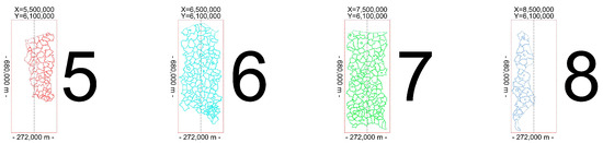
Figure 4.
Projection zone partitioning.
It is important to notice that the algorithm presented does not depend on the shape of boundaries of any spatial units, e.g., poviats. It uses the map sheet division in PL-2000 system, which covers the entire area of Poland within each zone (EPSG: 2176-2179). The example of map sheet division beneath irregularly shaped boundaries of selected poviats is presented in Figure 5.
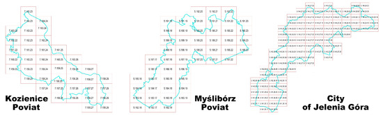
Figure 5.
Map sheet division beneath selected irregularly shaped poviats.
Edge-stability tests were conducted over the entire PL-2000 domain. A regular grid at the 1:500 sheet resolution was employed: the domain was covered with control points at fixed spacing dX = 400 m, dY = 250 m (Figure 6). In addition, randomized XY samples were generated. With ε-perturbation and half-open boundary rules applied, no inconsistencies were found between (i) the sheet code generated at each scale and (ii) the inverse check performed at the center of the extent returned by the code → extent function.
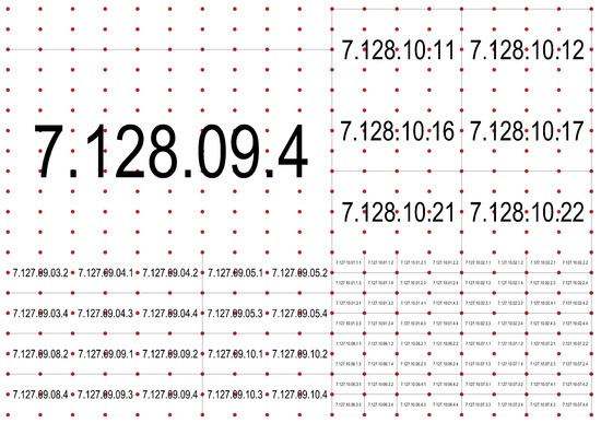
Figure 6.
Graphical illustration of the edge-stability test.
2.7. Transfer to Other National Reference Systems
The algorithm presented can be successfully transferred to any CRS which uses hierarchical map sheet division. The required elements that need to be taken into account are:
- The CRS extent—bounding box (including false northing/easting and axes definition);
- The base sheet dimensions and rules for further divisions into larger scales;
- A consistent boundary convention (half-open intervals with a small ε perturbation);
- A consistent rounding convention (floor) applied end-to-end.
To substantiate transferability beyond PL-2000, we refer to an independent, successful implementation for the archive Krakow Local Coordinate System [25]. Despite the different historical lineage (transformations to the Lviv cadastral frame), the arithmetic template is unchanged, demonstrating that the method is portable across distinct CRSs once the abovementioned components are provided.
3. Results
3.1. Time Performance and Memory Overhead
Benchmarks in VB6 (MicroStation CONNECT) on an Intel Core i3-10110U confirmed a baseline throughput of ~360k operations/s (no optimizations). Replacing string concatenation of the sheet code with writing to a numeric Long key eliminates text conversions and typically yields a further ~8–15% gain, i.e., ~400k operations/s in the same environment. Estimates for Python 3.12.3 (NumPy 2.3.5) and C/C++ (Microsoft Visual C++ 2019) indicate throughputs on the order of 1.0–1.5 million and 2–3 million operations/s, respectively, while preserving identical logic and edge stability. The throughput by environment is summarized in Table 3.
Table 3.
Throughput by environment.
The algorithm presented was also compared against other existing spatial indexing strategies. These are Uber’s H3, Google’s S2, and Geohash. We include both the table with time complexity and space complexity in Big(O) notation (Table 4), and the summary with benchmarks for time and memory performed with the selected algorithms in the Python environment (Table 5).
Table 4.
Comparison of time complexity and space complexity of selected algorithms in the Big(O) notation.
Table 5.
Benchmarks on time and memory for the selection of the algorithms.
The computational tests were run for 1:500 sheets in PL-2000, and compared against H3 resolution = 9 [11], S2 level = 14 [10], and Geohash precision = 7 [15] to ensure as-similar-as-possible areas of cells. There were 1,699,375 points within the dataset.
The analyses show that for selected spatial resolutions, the proposed PL-2000 indexer reaches a median 3.16 M pts/s, outperforming H3 (resolution = 9) by ~5×, Geohash (precision = 7) by ~30×, and S2 (level = 14) by ~50× on the same dataset. RSS Δ = 0.02 MiB indicates negligible method-specific memory overhead for PL-2000, whereas H3 shows the largest delta (~114 MiB), which is probably caused by reprojection buffers and string/ID allocations. The higher RSS peak observed for PL-2000 reflects holding large NumPy input arrays (X,Y) and preparing the int64 output vector at the same time. The analysis confirm the robustness of the presented algorithm.
3.2. Implementation Comparison
VB6 remains sufficiently performant for integration with existing engineering toolchains (e.g., MicroStation CONNECT) at low migration cost. Python (with NumPy) performs well for batch jobs and prototyping, offering a favorable readability–performance trade-off. C/C++—owing to compilation and fine-grained control of CPU caching—achieves the highest throughput and is preferred for real-time services or very large-scale processing.
3.3. Potential Applications and Expected Benefits
This subsection outlines potential applications of the sheet code in typical processing streams. The descriptions are conceptual (no controlled empirical tests are reported here); the aim is to indicate potential benefits, risks, and minimal implementation steps.
3.3.1. LiDAR (Target Scale 1:2000)
Idea: assign a sheet code to every point at import to enable per-sheet partitioning and processing.
Potential workflow: (1) code assignment → (2) per-sheet sorting/partitioning → (3) de-duplication within a sheet → (4) filtering and height computations on small, homogeneous batches → (5) merge results.
Expected benefits: reduced I/O (local operations), simple parallel task splitting, reproducible assignment, and straightforward quality metrics (density, gaps, deviations) per sheet.
Risks/assumptions: edge effects (recommend a processing buffer), mixed epochs/frames (normalization required), duplicate-resolution rules between point clouds.
Minimal prototype: one administrative unit; compare time and I/O cost with/without per-sheet partitioning.
3.3.2. Orthophoto (Target Scale 1:5000)
Idea: per-sheet indexing yields deterministic tile names and enables incremental rendering.
Potential workflow: (1) map scenes to sheets → (2) build tiles named by the sheet code → (3) update by rendering only changed tiles → (4) distribute via cache/CDN.
Expected benefits: shorter rebuilds (recompute only “touched” tiles), improved cache hit rates, transparent coverage/gap reporting.
Risks/assumptions: tile seams (overscan/border), consistent resampling rules, georeferencing accuracy control at sheet edges.
Minimal prototype: one county (poviat); measure time needed to leave the tile and rebuild it with/without per-sheet indexing.
3.3.3. Hyperspectral Data (Target Scale 1:10,000)
Idea: use the sheet code as a common join key with vector masks and areas of interest (AOIs).
Potential workflow: (1) assign cubes/bands to sheets → (2) cut by masks within a sheet → (3) compute indices/classifications per sheet → (4) merge results and coverage statistics.
Expected benefits: constrain costly spatial queries to small subsets, reduce memory overhead, enable natural parallelism.
Risks/assumptions: spectral consistency at boundaries (buffer), harmonization of NODATA values, resampling costs when changing resolution.
Minimal prototype: several adjacent 1:10,000 sheets; compare mask-join time versus classical spatial queries.
3.3.4. Implications for GeoAI
- Multi-scale solution: change resolution by truncating trailing code symbols (e.g., 1:500 → 1:1000 → 1:2000 → 1:10,000) without recomputing geometry.
- Easier training and inference: stable sampling/stratification by code (training); fast routing of data chunks to the proper per-sheet model (online inference).
- More effective data engineering: per-sheet table partitions, numeric-key indexes, code-based manifests (eases versioning and CI/CD).
- Tool for quality control: per-sheet metric dashboards (counts, density, NODATA, duplicates, edge error) with simple alert thresholds.
4. Discussion
Replacing classical topological queries (e.g., point-in-polygon) with constant-time O(1) arithmetic simplifies the ETL pipeline and reduces dependency on exact boundary geometries. Adding a sheet code/identifier column slightly increases the record size, but it facilitates filtering, partitioning, and joins. The choice between on-the-fly code computation and materializing a column should follow the workload profile: query frequency, I/O throughput, memory budget, and reproducibility requirements. In read-heavy systems, materialization typically lowers total cost; in high-throughput transactional streams, computing codes on the fly may be preferable.
It is worth noting that the solution is flexible and can be joined with other approaches. Global indexing grids (DGGS, S2/H3) provide planet-wide uniformity and favorable computational properties, but they require reprojection and do not reflect the national semantics of cartographic sheet hierarchies. Tree structures (e.g., R-tree, quadtree) are universal and flexible, yet their logarithmic cost and reliance on boundary geometries and index maintenance can be less attractive when bulk-classifying records into a fixed, statutory sheet grid. The approach presented here is complementary: it complies with the national cartographic standard and can coexist with global indices in hybrid architectures (e.g., a sheet-code column alongside a parallel S2/H3 index for cross-system queries) [18].
The strategy is portable to other national systems, provided a formal, hierarchical sheet partition exists or can be unambiguously defined from metric parameters and boundary rules. Under these conditions, sheet codes serve as deterministic spatial indices that can be mapped to numeric keys and used in ETL, tiled services (TMS), and GeoAI tasks (sampling, routing data to models, multi-scale aggregation). It is also possible to adapt the algorithm for larger scales. For ETL/cache/GeoAI needs, sheets can be refined recursively via additional 2 × 2 splits below 1:500 (e.g., technical LOD levels 1:250, 1:125, etc.). This does not change the semantics of official sheets—treat these as extra LOD levels within the parent sheet. Upward aggregation is trivial (integer division by 4k).
Main limitations which might be noticed are associated with the scope and specifics of 1:5000 partition. The method assumes PL-2000 and formal sheet-coding rules. The 1:5000 path forms a parallel branch relative to the sequence 1:10,000 → 1:2000 → 1:1000 → 1:500 (for 1:10,000 we split 2 × 2; for 1:2000 we split 5 × 5). Because 1:5000 and 1:2000 boundaries do not coincide, transitions between branches require an intermediate pivot level— 1:1000. Also, technical constraints due to high resolution of some datasets may appear. Mitigation strategies may include the following: (1) compression and streaming/paging; (2) buffering at sheet boundaries; and (3) applying consistent boundary rules (half-open intervals + a small ε perturbation) to ensure stable assignment. Furthermore, mixed epochs/CRS versions, boundary updates, and reprojection errors introduce small shifts and inconsistencies. When consolidating multiple sources, uncertainties accumulate—especially at sheet edges and when crossing branch boundaries (1:5000 ↔ 1:2000). These risks are mitigated by CRS/epoch harmonization, a reference boundary version, and a consistent boundary rule.
We identify several possible future research directions, which may include the following:
- Integration with reference libraries (C++/Python/SQL) with unambiguous boundary rules, a pivot level, and 2 × 2 LOD support.
- Integration into the DGGS framework for supporting interoperability with global infrastructures.
- Development of code validators and public test suites (edge, inter-branch, and multi-level LOD cases).
- Conducting case studies for other national systems and portability assessment.
- Transferring the algorithm for use with the IMW reference system.
- Performing cost–benefit analyses in hybrid architectures (coexistence with S2/H3).
- Performing thorough analyses focused on integration with polygon operations, buffering, large-scale spatial joins, and other geoprocessing operations.
- Formulating guidelines for buffering and multi-scale processing of very-high-resolution data, including the impact of hierarchy depth k (levels) on bit budget and performance.
5. Conclusions and Recommendations
This paper presents a novel and efficient approach to spatial data indexing based solely on the rules of hierarchical map sheet division in the PL-2000 CRS (EPSG: 2176, 2177, 2178 and 2179). By formulating the forward (XY → code) and inverse (code → extent) procedures as purely arithmetic operations, we demonstrated that the entire system can be indexed in constant time O(1), without the need for geometric operations or search structures. The approach can be easily transferred to other national CRSs which incorporate hierarchical map sheet logic.
Benchmarks on time and memory clearly indicate that the method performs comparably to contemporary global indexing systems such as H3, S2, and Geohash while preserving full compatibility with national mapping standards. Achieving O(1) indexing is particularly significant as it confirms the suitability of the algorithm for using in spatial ETL, tile services, and remote sensing workflows while ensuring lower computational cost, as pure arithmetic is used instead of topological operations. It accelerates the indexing process, and eliminates dependencies on external libraries, e.g., for geometry processing. In practice, data pipeline architecture is based on a fixed-cost operation whose complexity does not grow with dataset size, and the algorithm is stable over entire CRS extent, including boundary regions owing to incorporating small ε perturbation), predictable, scalable, and allows for easy integration into GeoAI or network services. The key findings can be listed as follows:
- The XY → code and code → extent algorithms operate in constant time O(1), simplifying the organization and access to nationwide remote sensing data and reducing reliance on costly topological operations.
- The hierarchical PL-2000 structure supports multi-scale aggregation and decomposition without changing data structures, while compliance with national sheet rules facilitates institutional adoption.
- Sheet codes provide a stable partitioning/versioning key for AI pipelines (training, inference) and network services (TMS/OGC Tiles).
- Unified boundary rules (half-open intervals plus a small ε perturbation) ensure deterministic behavior at boundaries and stable resolution switching providing operational consistency.
Nevertheless, this study has its limitations. The main limitation is related to the static definition of the PL-2000 CRS with fixed-sheet geometry. Hence, it does not ensure coverage for the entire globe. Furthermore, although the algorithm itself is O(1), its practical usage still depends on upstream coordinate transformations when data arrives in geographic CRS.
From a practical perspective, transferring the approach to other national CRSs requires consideration of several implementation guidelines:
- For frequently queried datasets, materialize and index the sheet code/key column; this supports further gains in filtering, joins, and sharding.
- Mirror the code hierarchy in folder layouts and database schemas (file nomenclature, per-sheet partitions).
- In the case of PL-2000, treat 1:5000 as a separate branch; for inter-branch joins, use a pivot at 1000.
- Harmonize CRS and epoch, apply consistent boundary rules, and run per-sheet QA (density, gaps, seams).
- For very-high-resolution data plan for compression, streaming/paging, and buffering at sheet boundaries; if needed, add extra 2 × 2 LOD levels in the arithmetic hierarchy.
This research provides a strong foundation for future research. The main ones include integrating into a DGGS framework, developing reference libraries in C++, Python, SQL, and creating open-source libraries to support widespread adoption. Furthermore, cost–benefit analyses in coexistence with other leading spatial indexing systems could be performed. Large-scale evaluations on the complete Polish orthophoto and LiDAR archives would provide valuable operational validation. We also plan to assess the portability of the algorithm by adapting it for the entire globe by using the International Map of the World (IMW) reference system.
To sum up, the presented method for spatial indexing based on the national grid for map sheet division allows for operating in constant time (O1), which offers undoubtable practical values for contemporary geospatial pipelines. Its simplicity and reliance solely on arithmetic make it a practical and robust alternative to other, more complex global indexing systems.
Supplementary Materials
The following supporting information can be downloaded at: https://www.mdpi.com/article/10.3390/app152412915/s1, pseudocodes of the algorithms (VB6-friendly), full implementation notes for MicroStation.
Author Contributions
Conceptualization, M.Z.; methodology, M.Z.; software, M.Z.; validation, M.Z. and M.R.; formal analysis, M.Z. and M.R.; investigation, M.Z. and M.R.; resources, M.Z. and M.R.; data curation, M.Z. and M.R.; writing—original draft preparation, M.Z.; writing—review and editing, M.R.; visualization, M.Z. and M.R.; supervision, M.Z.; project administration, M.Z.; funding acquisition, M.Z. All authors have read and agreed to the published version of the manuscript.
Funding
This research was funded with a subsidy from the Ministry of Science and Higher Education for the University of Agriculture in Krakow and by the AGH University of Krakow research subsidy no. 16.16.150.545. The APC was with a subsidy from the Ministry of Science and Higher Education for the University of Agriculture in Krakow, with IOAP discount applicable for the AGH University of Krakow.
Institutional Review Board Statement
Not applicable.
Informed Consent Statement
Not applicable.
Data Availability Statement
The original data presented in this study (algorithms developed) are openly available in Supplementary Materials to this manuscript.
Conflicts of Interest
The authors declare no conflicts of interest. The funders had no role in the design of this study; in the collection, analyses, or interpretation of data; in the writing of the manuscript; or in the decision to publish the results.
Abbreviations
The following abbreviations are used in this manuscript:
| DGGS | Discrete Global Grid Systems |
| OGC | Open Geospatial Consortium |
| I/O | Input/Output |
| TMS | Tile Matrix Set |
| ETL | Extract, Transform, Load |
| BSTR | Basic (Binary) String |
| DBMS | Database Management System |
| AI | Artificial Intelligence |
| VB6 | Visual Basic 6.0 |
| SQL | Spatial Query Language |
| LiDAR | Light Detection and Ranging |
| LOD | Level of Detail |
| CRS | Coordinate Reference System |
| QA | Quality Assessment |
References
- Goodchild, M.F. Reimagining the history of GIS. Ann. GIS 2018, 24, 1–8. [Google Scholar] [CrossRef]
- Sahr, K.; White, D.; Kimerling, A.J. Geodesic discrete global grid systems. Cartogr. Geogr. Inf. Sci. 2003, 30, 121–134. [Google Scholar] [CrossRef]
- Mahdavi-Amiri, A.; Samavati, F.; Peterson, P. Categorization and conversions for indexing methods of discrete global grid systems. ISPRS Int. J. Geo-Inf. 2015, 4, 320–336. [Google Scholar] [CrossRef]
- Mahdavi-Amiri, A.; Alderson, T.; Samavati, F. Geospatial data organization methods with emphasis on aperture-3 hexagonal discrete global grid systems. Cartographica 2019, 54, 30–50. [Google Scholar] [CrossRef]
- Koh, K.; Hyder, A.; Karale, Y.; Kamel Boulos, M.N. Big Geospatial Data or Geospatial Big Data? A Systematic Narrative Review on the Use of Spatial Data Infrastructures for Big Geospatial Sensing Data in Public Health. Remote Sens. 2022, 14, 2996. [Google Scholar] [CrossRef]
- Li, S.; Dragicevic, S.; Anton, F.; Sester, M.; Winter, S.; Coltekin, A.; Pettit, C.; Jiang, B.; Haworth, J.; Stein, A.; et al. Geospatial big data handling theory and methods: A review and research challenges. ISPRS J. Photogramm. Remote Sens. 2016, 115, 119–133. [Google Scholar] [CrossRef]
- Open Geospatial Consortium (OGC). OGC API—Tiles—Part 1: Core (OGC 20-057), Version 1.0.0; Approved 10 November 2022. Available online: https://docs.ogc.org/is/20-057/20-057.html (accessed on 25 September 2025).
- Open Geospatial Consortium (OGC). OGC Two-Dimensional Tile Matrix Set and Tileset Metadata, Version 2.0 (OGC 17-083r4). Available online: https://docs.ogc.org/is/17-083r4/17-083r4.html (accessed on 25 September 2025).
- S2 Geometry Library. Available online: https://s2geometry.io/ (accessed on 25 September 2025).
- H3: Hexagonal Hierarchical Geospatial Indexing System. Available online: https://h3geo.org/ (accessed on 25 September 2025).
- Open Geospatial Consortium (OGC). Topic 21: Discrete Global Grid Systems (DGGS). Available online: https://docs.ogc.org/as/15-104r5/15-104r5.html (accessed on 25 November 2025).
- ESRI. Introduction to Discrete Global Grid System (DGGS). Available online: https://ecce.esri.ca/blog/2023/06/24/introduction-to-discrete-global-grid-system-dggs/ (accessed on 25 November 2025).
- Kmoch, A.; Vasilyev, I.; Virro, H.; Uuemaa, E. Area and shape distortions in open-source discrete global grid systems. Big Earth Data 2022, 6, 256–275. [Google Scholar] [CrossRef]
- Movable Type Scripts. Geohash Algorithm Explained—How Geohash Works. Available online: https://www.movable-type.co.uk/scripts/geohash.html (accessed on 25 November 2025).
- Youngren, R.W.; Petty, M.D. A multi-resolution HEALPix data structure for spherically mapped point data. Heliyon 2017, 3, e00332. [Google Scholar] [CrossRef]
- Hobona, G.; Simmons, S.; Masó-Pau, J.; Jacovella-St-Louis, J. OGC API standards for the next generation of web mapping. Abstr. Int. Cartogr. Assoc. 2023, 6, 91. [Google Scholar] [CrossRef]
- Guttman, A. R-trees: A dynamic index structure for spatial searching. In Proceedings of the 1984 ACM SIGMOD International Conference on Management of Data (SIGMOD ’84), Boston, MA, USA, 18–21 June 1984; ACM: New York, NY, USA, 1984; pp. 47–57. [Google Scholar] [CrossRef]
- Finkel, R.A.; Bentley, J.L. Quad trees: A data structure for retrieval on composite keys. Acta Inform. 1974, 4, 1–9. [Google Scholar] [CrossRef]
- Samet, H. The quadtree and related hierarchical data structures. ACM Comput. Surv. 1984, 16, 187–260. [Google Scholar] [CrossRef]
- Zygmunt, M.; Gniadek, J.; Szewczyk, R. The method for setting map sheet identification numbers in the international map of the world (IMW) system. Geomat. Landmanag. Landsc. 2021, 1, 69–79. [Google Scholar] [CrossRef]
- Zygmunt, M.; Michałowska, K.; Ślusarski, M. The point location problem on the example of determining map identification number and map sheet extent in the IMW system. Geomat. Landmanag. Landsc. 2023, 1, 31–46. [Google Scholar] [CrossRef]
- Rada Ministrów. Rozporządzenie z Dnia 15 Października 2012 r. w Sprawie Państwowego Systemu Odniesień Przestrzennych. Dziennik Ustaw 2012, poz. 1247. Available online: https://isap.sejm.gov.pl/isap.nsf/DocDetails.xsp?id=WDU20120001247 (accessed on 25 September 2025).
- EPSG Geodetic Parameter Dataset. ETRF2000-PL/CS2000: EPSG:2176; 2177; 2178; 2179. Available online: https://epsg.io/2176 (accessed on 25 September 2025).
- Harrie, L.; Touya, G.; Oucheikh, R.; Ai, T.; Courtial, A.; Richter, K.-F. Machine learning in cartography. Cartogr. Geogr. Inf. Sci. 2024, 51, 1–19. [Google Scholar] [CrossRef]
- Zygmunt, M. Spatial indexing in access to cartographic archives for GIS/AI systems: A case study of ULK (Krakow Local System). Geomat. Landmanag. Landsc. 2025, 3, 131–146. [Google Scholar] [CrossRef]
- Uber. H3: Hexagonal Hierarchical Geospatial Indexing System. GitHub Repository. Available online: https://github.com/uber/h3 (accessed on 25 November 2025).
- Google. S2 Geometry Library. GitHub Repository. Available online: https://github.com/google/s2geometry (accessed on 25 November 2025).
- Overmars, M.H. Geometric data structures for computer graphics: An overview. In Theoretical Foundations of Computer Graphics and CAD; Earnshaw, R.A., Ed.; NATO ASI Series (Series F: Computer and Systems Sciences); Springer: Berlin/Heidelberg, Germany, 1988; Volume 40. [Google Scholar] [CrossRef]
Disclaimer/Publisher’s Note: The statements, opinions and data contained in all publications are solely those of the individual author(s) and contributor(s) and not of MDPI and/or the editor(s). MDPI and/or the editor(s) disclaim responsibility for any injury to people or property resulting from any ideas, methods, instructions or products referred to in the content. |
© 2025 by the authors. Licensee MDPI, Basel, Switzerland. This article is an open access article distributed under the terms and conditions of the Creative Commons Attribution (CC BY) license (https://creativecommons.org/licenses/by/4.0/).