Abstract
Subsea environments are vital for global biodiversity, climate regulation, and human activities such as fishing, transport, and resource extraction. Accurate mapping and monitoring of these ecosystems are essential for sustainable management. Airborne LiDAR bathymetry (ALB) provides high-resolution underwater data but produces large and complex datasets that make efficient analysis challenging. This study employs deep learning (DL) models for the multi-class classification of ALB waveform data, comparing two recurrent neural networks, i.e., Long Short-Term Memory (LSTM) and Bidirectional LSTM (BiLSTM). A preprocessing pipeline was developed to extract and label waveform peaks corresponding to five classes: sea surface, water, vegetation, seabed, and noise. Experimental results from two datasets demonstrated high classification accuracy for both models, with LSTM achieving 95.22% and 94.85%, and BiLSTM obtaining 94.37% and 84.18% on Dataset 1 and Dataset 2, respectively. Results show that the LSTM exhibited robustness and generalization, confirming its suitability for modeling causal, time-of-flight ALB signals. Overall, the findings highlight the potential of DL-based ALB data processing to improve underwater classification accuracy, thereby supporting safe navigation, resource management, and marine environmental monitoring.
1. Introduction
Oceans and seas cover approximately 75% of the Earth’s surface and act as the planet’s largest carbon sink, absorbing over 90% of excess heat generated by human activities [1]. They are vital for global trade, food security, and energy supply, yet our understanding of their topography remains limited. To date, only about one-quarter of the global seafloor has been mapped at high resolution, constraining scientific knowledge of underwater habitats and increasing risks for maritime navigation and resource management [2]. Comprehensive and accurate mapping of subsea environments is therefore critical for monitoring marine ecosystems, supporting sustainable resource utilization, and ensuring safe operations [3].
Recent technological advances in remote sensing have enhanced the potential for detailed underwater mapping. Among these technologies, Airborne LiDAR Bathymetry (ALB) has emerged as a powerful tool for surveying shallow and coastal waters [4,5]. Bathymetric LiDAR systems can measure depths up to 50 m (under perfect conditions) below the water surface, mapping the environment in the form of a dense point cloud [6]. As shown in Figure 1, ALB emits green laser light (typically at 532 nm), which is capable of penetrating the water column, capturing dense, high-resolution waveform data that reflect interactions with the sea surface, vegetation, and seabed structures. However, the immense volume and complexity of ALB waveform data represent significant challenges for automatic analysis. Each laser pulse generates thousands of intensity samples, which must be interpreted to distinguish different underwater targets, a process that remains largely dependent on manual or semi-automated methods.
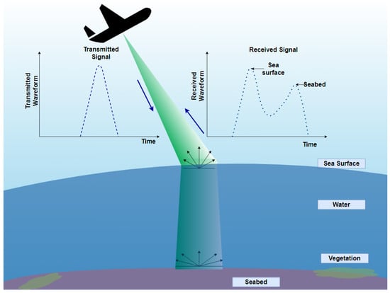
Figure 1.
Illustration of green laser transmission and interaction with underwater surfaces in bathymetric LiDAR scanning.
Conventional ALB processing methods, such as Gaussian decomposition or feature-based classification, often simplify or discard important waveform information, leading to reduced accuracy and limited generalization across varying environmental conditions, including water turbidity, depth, and surface motion [5,7,8,9]. A systematic literature review conducted by the authors in [10] revealed that most existing studies employ classical machine learning or shallow neural networks, including Multilayer Perceptrons (MLPs) [7,11,12], Convolutional Neural Networks (CNNs) [13,14], Random Forests [15,16], and Support Vector Machine (SVM) [17], often applied to preprocessed waveform segments. These methods have achieved high accuracy in seabed object detection [12], binary classification of ALB data [13], seafloor mapping [16], estimating the flow resistance characteristics [18], determining the sea level and seafloor [14], seabed modeling with oversampling [12], voxel-based semantic segmentation [19], and bottom-type characterization [17]. Nevertheless, they generally rely on handcrafted features, partial waveform segments, and site-specific calibration, limiting their applicability to diverse marine environments. Furthermore, the potential of full-waveform data, particularly temporal signal characteristics such as rise and decay times, remains underexplored, as does the application of advanced Deep learning (DL) architectures capable of capturing sequential dependencies in ALB waveform data.
To address these gaps, this study investigates the application of the Recurrent Neural Networks (RNNs), particularly Long Short-Term Memory (LSTM) and Bidirectional LSTM (BiLSTM) architectures, for the multi-class classification of ALB waveforms data into five subsea classes: sea surface, water, vegetation, seabed, and noise. This is because these models are well-suited to capture sequential dependencies in time-of-flight laser returns [20,21], but their application to full-waveform ALB data has not been systematically evaluated. In addition, a dedicated preprocessing and labeling framework was developed to preserve the full temporal and amplitude structure of waveforms, enabling models to learn directly from raw data. This study addresses the following research questions:
- RQ1: Which deep learning models perform best for multi-class classification of subsea classes on ALB waveform data?
- RQ2: How reliable is the classification of an individual bathymetric point for seabed and vegetation mapping?
- RQ3: How do deep learning models compare with existing approaches reported in the literature?
Overall, this study presents a comprehensive data-driven framework for accurate ALB waveform classification and evaluates model performance across diverse conditions. The remainder of this paper is structured as follows. Section 2 describes the research methodology, including data acquisition, preprocessing, and model architecture. Section 3 presents experimental results. Section 4 provides a discussion. Finally, Section 5 concludes this study with insights and future research directions.
2. Materials and Methods
This section presents the overall methodology, starting with an overview of the proposed solution in Section 2.1, which consists of several stages. The first stage covers data collection and its description in Section 2.2, followed by the data preparation phase in Section 2.3. The third stage addresses data preprocessing, including data labeling, noise filtering, data normalization, and data splitting for model training in Section 2.4. The network architectures utilized in the study are then described in Section 2.5. Finally, the evaluation metrics used to measure model performance are presented in Section 2.7.
2.1. Proposed Solution
To classify bathymetric LiDAR data into five classes—sea surface, vegetation, seabed, water, and noise—a generic solution was developed, as illustrated in Figure 2. The process began with data collection, where two datasets were gathered. This was followed by a comprehensive workflow that included data preparation and a data preprocessing pipeline applied to both datasets. The data was then split into training, validation, and testing datasets. Subsequently, two deep learning models were trained, and the hyperparameters were selected empirically based on preliminary experiments and validation performance. The following subsections describe each step in detail.
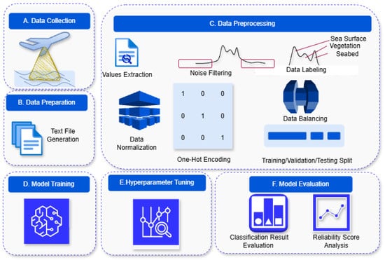
Figure 2.
The step-by-step process of the proposed solution.
2.2. Dataset and Description
In the proposed solution, the first step was data collection, as illustrated in Figure 2. This study utilized two Bathymetric LiDAR waveform datasets, which will be referred as Dataset 1 and Dataset 2. These datasets were collected by the Norwegian Mapping Authority (Kartverket) [22] and given to the author of this study. These datasets were collected from two test sites in a coastal area of Fjøløy Island, Norway. The map of the test area is shown in Figure 3, where the first dataset is marked in a blue rectangle and the second dataset is marked in a red rectangle. In the collected dataset, each waveform consisted of 960 discrete intensity samples representing the laser’s return, accompanied by metadata including geographic coordinates, sensor position, and time stamps. These waveforms formed the raw input for the classification task.
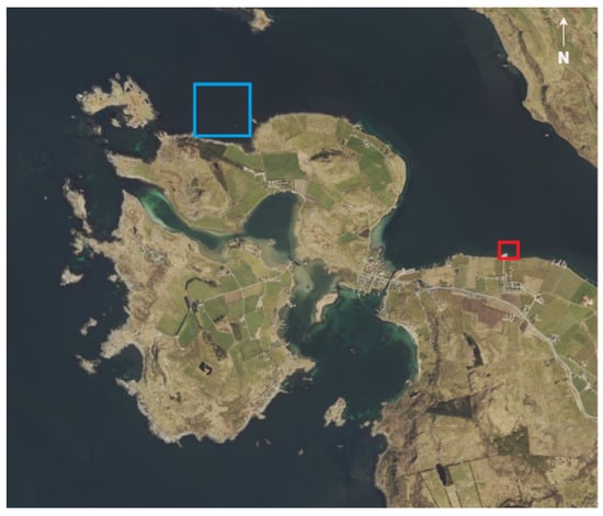
Figure 3.
Data collection locations.
2.3. Dataset Preparation and Merging
In the proposed solution, the second step was data preparation. The collected bathymetric LiDAR data comprises 3 different data files, which are: Trajectory, Project, and Waveform [23]. The Trajectory file contains the LiDAR sensor’s positional and orientation data, including latitude, longitude, altitude, and trajectory path recorded during data collection. The Project file stores metadata, system settings, and acquisition parameters such as scan resolution, scan density, and project-specific configurations that define the context of the LiDAR survey. The Waveform file includes information about the laser return signals, specifically the shape, amplitude, and timing of each waveform, providing insights into the surface characteristics and structure of the scanned environment [23].
To further proceed towards analysis, these three data files were converted into readable text format. This conversion was accomplished using MicroStation (https://www.bentley.com/software/microstation/ accessed on 24 August 2024) (Bentley Systems version 23.00.01.44), a CAD software platform that efficiently handles 2D and 3D point cloud data. By adopting this platform, the three types of files were merged into single, consolidated text files. After merging the text files, in total, there were 6379 text files contained in Dataset 1, and 4428 text files in Dataset 2, depicting one file for each laser return.
The excerpt of a text file from Dataset 1, ‘waveform_303371215_085609_only.txt’, is shown in Figure 4. The text file contains several fields describing the recorded waveform data. The field “Point” represents the first three values corresponding to the Cartesian coordinates of the reflecting point—east, north, and height. The second field, “Scanner”, lists the next three values (line 2), which describe the position of the scanner during data capture, specified by its coordinates (X, Y, Z). The “Intensity” field indicates the strength of the laser return for the given point (in this case, 301). The “Time (absolute GPS time, unit: sec)” field denotes the timestamp when the data was captured. The “Channel 1 Count” (here = 960) specifies the number of returns detected for Channel 1. The “Sample Length” field represents the time interval between consecutive sample points. The “Point” value indicates the elapsed time (in seconds) from the first recorded intensity sample to the return point within the waveform. The “Vector Information” field (lines 8–10) lists three values corresponding to the directional components (X, Y, Z) of the return vector. Finally, the “Channel 1 Samples” field contains a sequence of numeric values representing the intensity samples from Channel 1. Each file includes 960 intensity samples.
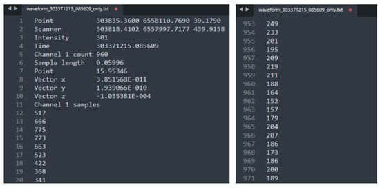
Figure 4.
The excerpt of a text file from Dataset 1.
The intensity values shown in the Text File ‘waveform_303371215_085609_only.txt’ are presented in the graphical form in Figure 5 for better illustration. Here, the x-axis represents the sample number (960 samples), while the y-axis represents the intensity values. In the figure, it can be seen that there are 3 visible peaks, which correspond to three key features that are depicted by the laser. The first peak value was considered as the sea surface, the second peak value was considered as vegetation, and the final peak value was considered as the seabed.
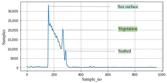
Figure 5.
Marked Peaks of the file ‘waveform_303371215_085609_only.txt’.
2.4. Data Preprocessing
This represents the third step in the proposed solution (Figure 2), which outlines the preprocessing workflow used to prepare the data for training the selected deep learning models, including detailed procedures for noise filtering, data labeling, and other necessary preprocessing tasks.
2.4.1. Values Extraction
In this step, numeric values from metadata were extracted. As illustrated in Figure 4, each text file contained metadata about the sensor and location, followed by 960 intensity samples. In the preprocessing stage, the metadata was separated from the numerical values for each text file, retaining only the data related to intensity samples.
2.4.2. Noise Filtering
After extracting the intensity values from the metadata, the next step in the data preprocessing was noise filtering. Removing noise is essential to enhance the quality of the analysis [24]. As each text file contained 960 samples of intensity values, the initial points before the sea surface and the points after the seabed were considered noise. The selection of these noise thresholds was made after discussing with the domain experts. Therefore, the first 100 and the last 560 values were identified as noise (highlighted with red boxes in Figure 6) and subsequently removed, keeping only the samples in the range of 101 to 400. This resulted in 300 intensity values instead of 960 values for each waveform.
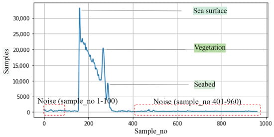
Figure 6.
Noise Filtering: The intensity values at the beginning (Sample_no 1–100) and at the end (Sample_no 401–960) were marked as noise (see marked red boxes).
These thresholds were chosen because they consistently preserved the complete valid signal region across all waveforms in both datasets. The early samples mainly contain sensor-level noise prior to the air–water interface, while the trailing samples correspond to attenuated energy occurring after the seabed return. Although heuristic in form, this range reflects the expected physical behavior of ALB full-waveform signals and was confirmed through repeated visual inspection and expert consultation.
2.4.3. Data Labeling
To classify ALB waveforms into distinct classes, peaks in the intensity profiles were detected using the ‘find_peaks’ function from the ‘SciPy’ library, and these detected peaks were used to delineate meaningful subsea classes. The first major peak was identified as the ‘sea surface’ and labeled as Class 1. The second class, ‘water’, corresponds to the region between the sea surface and vegetation, as well as the region between vegetation and the seabed, and was labeled as Class 2. The ‘vegetation’ class was characterized by intermediate peaks within the water column, preceding the seabed return, and was labeled as Class 3. The ‘Seabed’ class was defined by the final dominant reflection peak and was labeled as Class 4. Finally, samples falling outside the valid signal range were categorized as ‘Noise’ and labeled as Class 0. An example of a labeled waveform is shown in Figure 7 to understand the labeled classes for the file ‘waveform_303371215_085609_only.txt’.
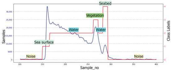
Figure 7.
Example of a labeled waveform (illustrated for the file ‘waveform_303371215_ 085609_only.txt’).
The assignment of these peaks is grounded in the physical behavior of ALB waveforms. The sea surface consistently produces the earliest and strongest return due to the sharp refractive contrast at the air–water interface. Submerged vegetation generates intermediate peaks because plant structures partially scatter and attenuate the laser pulse within the water column. The seabed produces the final dominant return, representing the deepest reflective surface encountered by the pulse. These distinctions were validated through repeated inspection of waveform shapes across both datasets.
Although global noise outside the 101–400 sample window was removed in the previous preprocessing step, small irregular fluctuations may still occur inside the clipped region. These samples do not correspond to any physical return (sea surface, water, vegetation, or seabed) and are therefore labeled as ‘Noise’ (Class 0) to capture residual non-physical variations within the valid waveform segment.
After labeling the data, the total number of samples in each class for both datasets is presented in Table 1. From the table, it can be seen that the ‘Noise’ class contains 1,072,781 samples in Dataset 1 and 754,099 samples in Dataset 2. Whereas, class ‘sea surface’ contains 101,809 in Dataset 1 and 70,848 in Dataset 2. Class ‘water’ contains 615,134 samples in Dataset 1 and 450,087 samples in Dataset 2. The ‘vegetation’ class contains 53,863 in Dataset 1 and 4658 samples in Dataset 2. Finally, ‘seabed’ has 70,113 samples in Dataset 1 and 48,708 samples in Dataset 2.

Table 1.
Classes distribution between two datasets.
2.4.4. Data Normalization
For model input, the intensity values were treated as sequential features, and the corresponding classes as target labels. Each ALB waveform represents a time-of-flight sequence, where the intensity values change over time as the laser interacts with the sea surface, water column, vegetation, and seabed. Treating them as sequential data enables the model to learn these temporal variations during the classification process.
The ‘StandardScaler’ class from the ‘Scikit-learn’ library was used to normalize the feature data. This scaler removed the mean and scaled the data to unit variance, which helped in speeding up the convergence of stochastic gradient descent.
2.4.5. One-Hot Encoding
Since the dataset contains five different classes, the labels were converted to a one-hot encoded format using the ‘to_categorical’ function from ‘tensorflow.keras.utils’. One-hot encoding transformed each label into a binary vector, where the index corresponding to the actual class was set to 1, and all other indices were set to 0. This transformation was necessary because the final output layer of the model was designed to predict class probabilities across multiple categories.
2.4.6. Data Balancing
The raw bathymetric LiDAR waveform dataset showed significant class imbalance across the five defined classes—noise, sea surface, water, vegetation, and seabed. As shown in Table 1, the majority of samples corresponded to noise and water returns, whereas vegetation and seabed classes were substantially underrepresented. Addressing this imbalance was essential to ensure that the deep learning models did not become biased toward the dominant classes. Rather than applying traditional oversampling techniques such as SMOTE, which may lead to overfitting due to the generation of synthetic points, the study implemented a class-weighting approach during model training. The ‘compute_class_weight’ function from ‘sklearn.utils.class_weight’was used to calculate proportional weights for each class based on its frequency in the training set. Higher weights were assigned to minority classes (particularly vegetation and seabed), ensuring that the loss function penalized their misclassification more strongly (see Table 2).

Table 2.
Computed weights on different classes.
The exceptionally large weight observed for Class 3 (vegetation) in Dataset 2 (56.73) arises directly from the extreme imbalance in this dataset: only 4658 vegetation samples were present compared to 754,099 noise samples and 450,087 water samples. Because the class-weighting scheme scales weights inversely with class frequency, this disparity produces a much larger weight for vegetation relative to other classes. Despite its magnitude, training remained stable due to the use of dropout regularization and early stopping, and the weight accurately reflects the scarcity of vegetation samples in Dataset 2.
2.4.7. Splitting Data into Training, Validation, and Testing Datasets
To build a fair and effective classification model, the datasets needed to be split into different sets for training, validation, and testing. A common approach involves setting aside 80% of the data for training the model, allowing it to learn and identify patterns in the data. The remaining 20% of the data was split equally, with 10% used for validation to adjust the model’s parameters and prevent overfitting, and 10% reserved for testing to evaluate the model’s performance. The ‘train_test_split’ function from ‘sklearn.model_selection’ was used to divide the normalized data into training and testing sets.
2.5. Network Architecture
Figure 8 depicts the network architecture used for multi-class classification of ALB waveform data. In this study, two recurrent neural network (RNN) architectures, such as Long Short-Term Memory (LSTM) and Bidirectional LSTM (BiLSTM), were employed. Both models were designed to process sequential waveform data by learning temporal dependencies between intensity peaks. The LSTM model captures causal dependencies—each sample depends only on preceding ones—while the BiLSTM extends this by processing sequences in both directions, enabling the evaluation of whether bidirectionality benefits ALB classification.
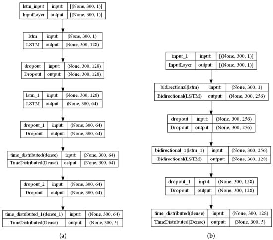
Figure 8.
The employed deep learning network architectures: (a) LSTM Model Architecture. (b) BiLSTM Model Architecture.
Each model consisted of two recurrent layers with 128 and 64 units, respectively, each followed by a dropout layer (rate = 0.5) to mitigate overfitting. The LSTM model additionally included a TimeDistributed Dense layer (64 units, ReLU activation) before the output layer. Both models concluded with a TimeDistributed Dense layer employing softmax activation for multi-class classification.
2.6. Experimental Setup and Hyperparameter Tuning
Table 3 provides a summarized comparison for both models, highlighting differences in the considered architecture, optimization for the classification task. From the table, it can be seen that the LSTM model was trained using the Adam optimizer (learning rate = 0.001) with a batch size of 32, while a smaller learning rate (learning rate = 0.0001) was used for the BiLSTM model with a batch size of 16. Both models were trained with 100 epochs, where early stopping was applied to prevent overfitting when there was no improvement observed in the validation loss. The categorical cross-entropy loss function and accuracy metric were used during training for multi-class classification and to evaluate the model performance, respectively.

Table 3.
Comparison between the structure and setup for the two models.
2.7. Model Performance Metrics
The final models’ performances were evaluated using key performance metrics, including overall accuracy [25,26], precision [25], recall [25,26], F1-score [25,26], and confusion matrices [25,26], to provide a comprehensive analysis of the predictive capabilities of the models. Additionally, confidence scores [27] were extracted for each classified point to quantify prediction reliability, with particular emphasis on distinguishing vegetation from seabed returns. Comparative analyses were performed across both datasets to evaluate model generalizability.
3. Results
This section presents the results obtained from two trained LSTM and BiLSTM models on two datasets. Each model was evaluated based on accuracy, precision, recall, and F1-score. Additionally, confidence scores were computed to examine prediction reliability for each class.
3.1. Experimental Results on the Dataset 1
Table 4 presents the results obtained from a series of experiments conducted on Dataset 1. From the table, it can be observed that LSTM obtained an overall accuracy of 95.22%, whereas the BiLSTM model got an overall accuracy of 94.37%.

Table 4.
The obtained results on two datasets using LSTM and BiLSTM.
For the LSTM, the macro-averaged precision, recall, and F1-score were 0.8787, 0.8594, and 0.8641, showing balanced performance across the classes. Although both models performed well, LSTM had slightly better overall accuracy and macro precision, meaning it kept a more even balance between precision and recall. The BiLSTM’s macro average recall (0.9486) was higher than the LSTM’s (0.8594), which means it found a larger share of the true positives but with lower precision. The LSTM, on the other hand, showed higher weighted-average recall (0.9522) and F1-score (0.9518), proving more reliable when dealing with class imbalance. Overall, both networks performed strongly, with LSTM showing a small advantage in generalization and balanced classification.
Figure 9 illustrates the confusion matrix analysis obtained from Dataset 1 using both LSTM and BiLSTM models. As shown in Figure 9a, the LSTM model shows strong classification performance, correctly identifying most samples across all classes. The majority of true labels, particularly the class 0 (209,814 instances) and class 1 (15,625 instances), were accurately predicted, reflecting high precision and recall for these classes. Misclassifications were relatively low and mainly occurred between classes with similar characteristics, such as class 3 and class 4. This pattern aligns well with the high overall accuracy (95.22%) and weighted F1-score (0.9518) reported in Table 4, confirming that the LSTM effectively learned the temporal dependencies within the dataset.
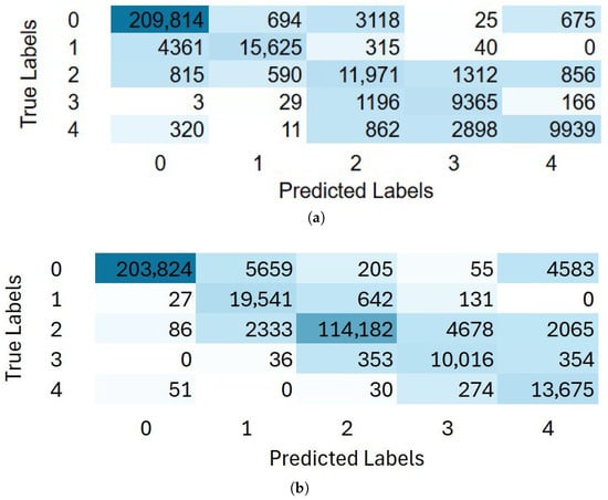
Figure 9.
The obtained confusion matrices on Dataset 1: (a) Confusion matrix using LSTM. (b) Confusion matrix using BiLSTM.
In contrast, Figure 9b shows that the BiLSTM model also achieved good performance but with slightly more misclassifications, particularly between classes 2 and 3. While the BiLSTM correctly classified the majority of samples in each class, for example, 203,824 instances for class 0 and 19,541 for class 1, it exhibited higher off-diagonal values compared to the LSTM. This suggests that the bidirectional architecture may have introduced noise or redundancy in sequential dependency learning, leading to reduced precision in certain classes. Despite its strong recall (macro-average of 0.9486), these misclassifications contributed to the slightly lower overall accuracy (94.37%) and weighted average F1-score (0.9478) compared to the LSTM. Overall, the confusion matrices confirm that both models performed robustly, but the unidirectional LSTM provided more consistent classification accuracy across all categories.
3.2. Experimental Results on the Dataset 2
Table 4 has the results obtained from the experiments conducted on Dataset 2. From the table, it can be observed that the LSTM model achieved a higher overall accuracy of 94.85% compared to the BiLSTM model with an overall accuracy of 84.18%, indicating that the unidirectional LSTM provided better generalization and stability on this dataset. In terms of macro-average metrics, the LSTM achieved a precision of 0.7011, a recall of 0.6885, and an F1-score of 0.6945, outperforming the BiLSTM in all three measures. This suggests that the LSTM was more effective at maintaining a balance between precision and recall across all classes. Although the BiLSTM obtained a relatively higher recall value of 0.8359, its much lower precision value of 0.6112 and F1-score of 0.635 indicate that it generated a large number of false positives, thereby reducing overall reliability.
The weighted-average results further confirm that the LSTM shows stronger performance, with a precision of 0.9446, recall of 0.9485, and F1-score of 0.9464, compared to the BiLSTM’s precision of 0.9482, recall of 0.8418, and F1-score of 0.8787, respectively. The higher weighted-average recall and F1-score of the LSTM demonstrate its consistent predictive performance. In contrast, the BiLSTM’s lower overall accuracy and variability across metrics suggest that the bidirectional architecture has struggled to capture the temporal dependencies effectively in this dataset. Overall, these results highlight that the LSTM architecture was better suited for Dataset 2, providing more accurate and stable predictions across all evaluation metrics.
The confusion matrix analysis, as shown in Figure 10, was obtained from Dataset 2 using the LSTM and BiLSTM models. As shown in Figure 10a, the LSTM model demonstrates strong classification performance, with most samples correctly predicted across the dominant classes. The majority of true labels—particularly Class 0 with 146,524 instances, Class 1 with 8886 instances, and Class 2 with 8824 instances—were accurately classified, indicating high precision and recall for these categories. However, Class 3 was not recognized, with most of its samples misclassified as Class 2 (785 instances) or Class 1 (127 instances), suggesting low separability due to overlapping waveform characteristics and limited representation in the dataset. This pattern aligns with the overall accuracy and weighted F1-score presented in Table 4, confirming that the LSTM effectively captured the temporal dependencies within the waveform data.
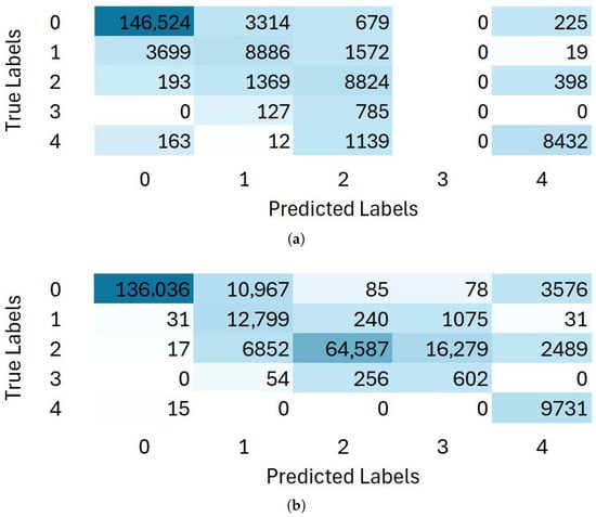
Figure 10.
The obtained confusion matrices on Dataset 2: (a) Confusion matrix using LSTM (b) Confusion matrix using BiLSTM.
In contrast, Figure 10b shows that the BiLSTM model also achieved good overall performance but exhibited more misclassifications compared to the LSTM. The BiLSTM model correctly classified the majority of samples, for example, 136,036 instances for Class 0 and 64,587 for Class 2, but it displayed higher off-diagonal values, particularly confusion between Classes 2 and 3 (16,279 instances). This suggests that while the bidirectional architecture improved context awareness, it may have introduced redundancy in sequence learning, slightly reducing precision for certain classes. Despite its strong recall (macro-average shown in Table 4), these misclassifications contributed to a marginally lower overall accuracy and F1-score compared to the LSTM.
The persistent misclassification of vegetation is primarily driven by its extremely low sample count relative to the dominant classes. In Dataset 2, for example, vegetation comprises only 4658 samples, whereas water contains 450,087. To address this imbalance, a class-weighting strategy was adopted, assigning substantially higher weights to the vegetation class (56.73) in the loss function. Although this technique increases the penalty for vegetation misclassification, the level of imbalance is so extreme that the model still lacks sufficient examples to learn a distinctive and generalizable waveform pattern. Consequently, vegetation returns are often absorbed into adjacent classes, particularly water, reflecting both the underlying class scarcity and the inherent similarity of their waveform signatures.
3.3. Results on Reliability Analysis Using Confidence Scores
To evaluate the reliability of classification for each sample, the confidence score was computed for the predicted classes.
This score represents the model’s certainty in assigning a specific label to a waveform segment. For illustration, Figure 11 presents the reliability analysis for a waveform (e.g., Text File 15) from Dataset 1 using both LSTM and BiLSTM models.
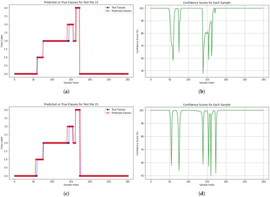
Figure 11.
The obtained confidence scores for a specific text file from Dataset 1 for reliability analysis: (a) True Class vs. Predicted Class using LSTM. (b) Confidence Score using LSTM. (c) True Class vs. Predicted Class using BiLSTM. (d) Confidence Score using BiLSTM.
Figure 11a,c compare the true and predicted class labels across 300 samples, where blue markers indicate ground-truth labels (true class) and red markers represent model predictions (predicted class). Overall, both models exhibit strong agreement between true and predicted classes, with most points overlapping. However, noticeable deviations occur around sample indices 130–160, corresponding to dips in the confidence score plots shown in Figure 11b,d.
The confidence score plots reveal that both models experience significant drops in certainty for these samples, with a minimum score of approximately 47% for LSTM and 50% for BiLSTM. While BiLSTM demonstrates slightly more stability during these dips, both models maintain high confidence for the majority of samples. These findings suggest that confidence scores provide a useful probabilistic measure of classification reliability, particularly for critical tasks such as seabed and vegetation mapping.
4. Discussion
The primary goal of this study was to evaluate the effectiveness of recurrent deep learning architectures, specifically LSTM and BiLSTM networks, for the multi-class classification of Airborne LiDAR Bathymetry (ALB) waveform data. In this context, the results obtained from these models were compared with existing approaches reported in the previous studies, as summarized in Table 5. Traditional machine learning models, such as Multilayer Perceptron (MLP), achieved accuracies ranging from 92.07% [7] to 97% [12] when combined with data balancing techniques like LVQ SMOTE, and ROSE [12]. However, other classical methods, such as Superpoint graph (SPG) [19], reported relatively lower accuracy, i.e., 72.45%, indicating limitations in handling complex feature dependencies present in high-dimensional signal data. Advanced architectures like MVCNN [13], and Transfer Learning models [18] demonstrated superior performance, achieving accuracies 99.41% and 95%, respectively. These results emphasize the strength of deep learning and feature extraction strategies in enhancing classification accuracy.
In comparison, the proposed LSTM and BiLSTM models achieved competitive results while maintaining architectural simplicity and interpretability. Specifically, the LSTM model obtained accuracies of 95.22% on Dataset 1 and 94.85% on Dataset 2, whereas the BiLSTM model achieved 94.37% and 84.18%, respectively. These findings confirm the suitability of recurrent architectures for sequential data, effectively modeling temporal dependencies inherent in waveform signals, without requiring extensive handcrafted features. However, the noticeable performance gap between Dataset 1 and Dataset 2 in the BiLSTM results suggests potential redundancy or overfitting introduced by the bidirectional processing, particularly when the dataset exhibits greater variability.
It is also important to recognize that the performance values in Table 5 originate from different datasets, sensors, and class definitions; therefore, these results serve as contextual reference points rather than direct baselines. A fair and controlled comparison with alternative deep learning frameworks, such as 1D CNNs, CNN–LSTM hybrids, multi-view CNNs, or Transformer-based sequence models would require training all models under identical preprocessing steps and class distributions. This work focused on evaluating temporal recurrent models as a first step toward full-waveform ALB classification, particularly due to their alignment with the causal time-of-flight behavior of laser returns. Future studies can build upon this foundation by systematically benchmarking these additional architectures under uniform experimental conditions.
When compared to highly specialized models such as MVCNN and RF, which reported near-perfect accuracies for specific classes (e.g., 100% water surface and 99% seabed [15]), our approach demonstrates robust generalization across multiple classes without relying on specialized feature engineering or object-level segmentation. This indicates that the temporal modeling alone can be sufficient for accurate multi-class waveform classification, providing an interpretable and computationally efficient alternative to more complex architectures.
Overall, while CNN-based and transfer learning approaches continue to dominate the state-of-the-art benchmarks in waveform classification, the LSTM-based models offer a balanced trade-off between accuracy, interpretability, and computational efficiency. These findings advance scientific understanding by demonstrating the capability of recurrent architectures to effectively model temporal dependencies, revealing the limitations of bidirectional processing under variable conditions, and establishing a benchmark for sequential waveform analysis. Moreover, the efficiency and simplicity of these models make them particularly suitable for real-time or resource-constrained applications, such as environmental monitoring or other geo-spatial remote sensing tasks. Collectively, these outcomes provide both theoretical and practical insights for the design and deployment of RNNs in sequential data classification.

Table 5.
Comparison of our work with the existing literature.
Table 5.
Comparison of our work with the existing literature.
| Literature Review | Used Models | Accuracy |
|---|---|---|
| [7] | MLP | 92.07% |
| [12] | MLP | 97.0%, with LVQ SMOTE, 96%, with ROSE |
| [19] | SPG | 72.45% |
| [13] | MVCNN | 99.41% |
| [15] | RF | 100% water surface, 99.9% seabed and 60% objects |
| [18] | Transfer Learning | 95% |
| [16] | KNN, SVM, RF | varies from 75% to 91% |
| Our Results | LSTM | Dataset 1: 95.22%, Dataset 2: 94.85% |
| BiLSTM | Dataset 1: 94.37%, Dataset 2: 84.18% |
Limitations of This Research
Despite these promising outcomes, several limitations must be acknowledged. First, the study did not explicitly incorporate environmental factors such as water turbidity, depth, and surface wave motion. These conditions can significantly influence the intensity and shape of ALB waveforms, potentially leading to signal overlap and misclassification [28]. Second, the difficulty observed in differentiating the seabed from vegetation is likely influenced by these unaccounted environmental factors. The lack of detailed metadata and integrated environmental measurements in the available datasets limited the ability to quantify how these factors contributed to classification errors or to establish direct relationships between signal distortions and classification accuracy. Incorporating such measurements in future research would enable a more comprehensive assessment of the physical and ecological determinants influencing ALB performance. Addressing these limitations in future studies will not only enhance model robustness but also foster a deeper understanding of the environmental and ecological drivers of uncertainty in ALB-based classification.
5. Conclusions
Airborne LiDAR Bathymetry (ALB) provides rich waveform data that can be used to classify key subsea features, including noise, sea surface, water, vegetation, and seabed. Accurate classification of these signals is critical for coastal mapping, environmental monitoring, and underwater resource management. Traditional methods rely on Gaussian decomposition or handcrafted point-based features, which can discard important temporal information inherent in the full waveform. In this study, two deep learning models were explored to leverage the full-waveform temporal structure, implementing LSTM and BiLSTM recurrent neural networks to perform multi-class classification directly on the waveform sequences.
The experimental results demonstrate that LSTM models consistently achieved high accuracy, i.e., more than 94% across both datasets. In contrast, BiLSTM models underperformed on Dataset 2, indicating that bidirectional processing does not enhance classification for time-of-flight governed ALB signals. These findings provide a scientific insight, i.e., causal sequence modeling aligns better with the physical principles of waveform generation, establishing that model selection should consider the underlying signal physics rather than relying solely on generic sequence learning architectures. Furthermore, the results highlight that vegetation and seabed classes remain challenging to distinguish due to environmental factors such as turbidity, water depth, and wave motion, which affect echo shapes and signal intensities.
These findings underscore the potential of recurrent neural networks, particularly LSTM, for robust subsea feature classification. By modeling the full waveform, our approach eliminates the need for manual feature engineering and demonstrates generalizability under varying environmental conditions and class imbalances. Importantly, the methodological advances, including a reproducible preprocessing and labeling pipeline, empirical evidence favoring causal temporal modeling, and an experimental design, provide a foundation for the practical deployment of ALB classification models.
Building on these findings, this study has demonstrated that artificial intelligence can classify ALB measurements using only the full waveform signal, unlike traditional Lidar classification approaches that rely on neighborhood analysis of point clouds. A key benefit of this approach is the ability to estimate a classification probability for each point, which is crucial for building trust in the final products. Trust in the classification results is a key factor for the full incorporation of ALB techniques into the production of nautical charts and operational seabed mapping campaigns. Therefore, this work represents a significant step toward integrating ALB into practical data acquisition workflows.
Future Work
This research shows that there is potential to further optimize and generalize deep learning for bathymetric classification. Future research directions may include:
Integration of environmental metadata: Future studies should integrate environmental parameters such as turbidity, water depth, salinity, and surface roughness to improve the model’s understanding of environmental dependencies that influence waveform characteristics. This integration could help address misclassifications between similar classes, such as vegetation and seabed, by providing contextual information about the physical environment and optical signal attenuation.
Multi-sensor fusion: Combining ALB data with other remote sensing modalities, such as hyperspectral imagery, sonar, or satellite optical data, can provide complementary information to enhance feature discrimination. Multi-sensor fusion could enable the model to capture both spectral and spatial cues, improving accuracy and robustness in heterogeneous underwater conditions.
Uncertainty quantification and interpretability: Implementing uncertainty-aware and interpretable modeling frameworks would improve the reliability of model predictions. Techniques such as Bayesian neural networks, attention-based visualization, or explainable AI (XAI) approaches could be used to estimate prediction confidence, interpret class boundaries, and identify the most influential waveform features. This would enhance the transparency and practical trustworthiness of the model in scientific and operational contexts.
Exploring advanced architectures: Further research could explore hybrid and transformer-based models that combine the strengths of LSTM/BiLSTM with attention mechanisms or convolutional layers. Such architectures may capture complex temporal-spatial dependencies more effectively, allowing for better representation of long-range waveform correlations. These models, paired with efficient training techniques and pruning strategies, could also reduce computational costs and enable real-time bathymetric classification.
In addition, a systematic evaluation of alternative deep learning baselines—such as 1D CNNs, CNN–LSTM hybrids, multi-view CNNs (MVCNN), and emerging architectures like Kolmogorov–Arnold Networks (KANs)—should be conducted using the same datasets and preprocessing pipeline presented in this study. This would enable direct and fair comparisons across model families and provide deeper insight into which architectures best capture the causal and physical dynamics of ALB waveform data.
Author Contributions
Conceptualization, N.T., H.G., V.N. and I.O.; methodology, N.T., H.G., V.N. and I.O.; software, N.T.; validation, N.T., V.N. and I.O.; formal analysis, N.T.; investigation, N.T.; data curation, N.T.; writing—original draft preparation, N.T.; writing—review and editing, N.T., H.G., V.N. and I.O.; visualization, N.T.; supervision, H.G., V.N. and I.O. All authors have read and agreed to the published version of the manuscript.
Funding
This research received no external funding.
Institutional Review Board Statement
Not applicable.
Data Availability Statement
The dataset used in this study, alongside the necessary scripts for model training, can be found in this GitHub repository: Classification of Bathymetric Data 2024. https://github.com/nabila22mumu/Classification-of-bathymetric-data-2024 (accessed on 10 January 2025).
Acknowledgments
N.T., H.G., V.N., and I.O. thank the Norwegian Mapping Authority for its support in providing resources and access to data, which have been instrumental in advancing this research. This study is the result of a 60-ECTS master’s thesis in Computer Science at the Department of Science and Industry Systems, Faculty of Technology, Natural Sciences and Maritime Sciences, University of South-Eastern Norway (USN), Kongsberg, Norway.
Conflicts of Interest
The authors declare no conflicts of interest.
Abbreviations
The following abbreviations are used in this manuscript:
| ALB | Airborne LiDAR Bathymetry |
| BiLSTM | Bidirectional Long Short-Term Memory |
| CNN | Convolutional Neural Network |
| DL | Deep Learning |
| KNN | K-Nearest Neighbour |
| LiDAR | Light Detection and Ranging |
| LSTM | Long Short-Term Memory |
| LVQ-SMOTE | Learning Vector Quantization based Synthetic Minority Oversampling Technique |
| MLP | Multi-Layer Perceptron |
| NMA | Norwegian Mapping Authority |
| RF | Random Forest |
| RNN | Recurrent Neural Network |
| SVM | Support Vector Machine |
References
- IFAW. How Climate Change Impacts the Ocean. 2024. Available online: https://www.ifaw.org/international/journal/climate-change-impact-ocean (accessed on 27 September 2025).
- World Ocean Review. Transport over the Seas. 2024. Available online: https://worldoceanreview.com/en/wor-7/transport-over-the-seas/ (accessed on 27 September 2025).
- American Scientist. An Ocean of Reasons to Map the Seafloor. 2023. Available online: https://www.americanscientist.org/article/an-ocean-of-reasons-to-map-the-seafloor (accessed on 4 September 2025).
- Pricope, N.; Bashit, M.S. Emerging trends in topobathymetric LiDAR technology and mapping. Int. J. Remote Sens. 2023, 44, 7706–7731. [Google Scholar] [CrossRef]
- Szafarczyk, A.; Toś, C. The Use of Green Laser in LiDAR Bathymetry: State of the Art and Recent Advancements. Sensors 2023, 23, 292. [Google Scholar] [CrossRef] [PubMed]
- 405nm. What is Airborne Lidar Bathymetry? 2023. Available online: https://405nm.com/what-is-airborne-lidar-bathymetry/ (accessed on 6 November 2025).
- Kogut, T.; Slowik, A. Classification of Airborne Laser Bathymetry Data Using Artificial Neural Networks. IEEE J. Sel. Top. Appl. Earth Obs. Remote Sens. 2021, 14, 1959–1966. [Google Scholar] [CrossRef]
- Dolan, M.; Buhl-Mortensen, P.; Thorsnes, T.; Buhl-Mortensen, L.; Bellec, V.; Bøe, R. Developing seabed nature-type maps offshore Norway: Initial results from the MAREANO programme. Nor. J. Geol. 2009, 89, 17–28. [Google Scholar]
- Leica Geosystems. Mapping Underwater Terrain with Bathymetric LiDAR. 2024. Available online: https://leica-geosystems.com/case-studies/natural-resources/mapping-underwater-terrain-with-bathymetric-lidar (accessed on 4 September 2024).
- Tabassum, N.; Giudici, H.; Nunavath, V. Exploring the Combined use of Deep Learning and LiDAR Bathymetry Point-Clouds to Enhance Safe Navigability for Maritime Transportation: A Systematic Literature Review. In Proceedings of the 2024 Sixth International Conference on Intelligent Computing in Data Sciences (ICDS), Marrakech, Morocco, 23–24 October 2024; pp. 1–5. [Google Scholar] [CrossRef]
- Deunf, J.L.; Mishra, R.; Pastol, Y.; Billot, R.; Oudot, S. Seabed prediction from airborne topo-bathymetric lidar point cloud using machine learning approaches. In Proceedings of the OCEANS 2021 San Diego–Porto, San Diego, CA, USA, 20–23 September 2021; IEEE: New York, NY, USA, 2021; pp. 1–9. [Google Scholar] [CrossRef]
- Kogut, T.; Tomczak, A.; Słowik, A.; Oberski, T. Seabed Modelling by Means of Airborne Laser Bathymetry Data and Imbalanced Learning for Offshore Mapping. Sensors 2022, 22, 3121. [Google Scholar] [CrossRef] [PubMed]
- Liang, G.; Zhao, X.; Zhao, J.; Zhou, F. MVCNN: A Deep Learning-Based Ocean–Land Waveform Classification Network for Single-Wavelength LiDAR Bathymetry. IEEE J. Sel. Top. Appl. Earth Obs. Remote Sens. 2023, 16, 656–674. [Google Scholar] [CrossRef]
- Zhong, J.; Sun, J.; Lai, Z.; Song, Y. Nearshore Bathymetry from ICESat-2 LiDAR and Sentinel-2 Imagery Datasets Using Deep Learning Approach. Remote Sens. 2022, 14, 4229. [Google Scholar] [CrossRef]
- Kogut, T.; Weistock, M. Classifying airborne bathymetry data using the Random Forest algorithm. Remote Sens. Lett. 2019, 10, 874–882. [Google Scholar] [CrossRef]
- Janowski, L.; Wroblewski, R.; Rucinska, M.; Kubowicz-Grajewska, A.; Tysiac, P. Automatic classification and mapping of the seabed using airborne LiDAR bathymetry. Eng. Geol. 2022, 301, 106615. [Google Scholar] [CrossRef]
- Eren, F.; Pe’eri, S.; Rzhanov, Y.; Ward, L. Bottom characterization by using airborne lidar bathymetry (ALB) waveform features obtained from bottom return residual analysis. Remote Sens. Environ. 2018, 206, 260–274. [Google Scholar] [CrossRef]
- Pan, S.; Yoshida, K. Using Airborne Lidar Bathymetry Aided Transfer Learning Method in Riverine Land Cover Classification. In Proceedings of the 14th International Symposium on Ecohydraulics, Nanjing, China, 10–14 October 2022. [Google Scholar]
- Roshandel, S.; Liu, W.; Wang, C.; Li, J. Semantic Segmentation of Coastal Zone on Airborne Lidar Bathymetry Point Clouds. IEEE Geosci. Remote Sens. Lett. 2022, 19, 1–5. [Google Scholar] [CrossRef]
- Wen, S.; Wang, T.; Tao, S. Hybrid CNN-LSTM Architecture for LiDAR Point Clouds Semantic Segmentation. IEEE Robot. Autom. Lett. 2022, 7, 5811–5818. [Google Scholar] [CrossRef]
- Rokon, O.F. RNN vs. LSTM vs. Transformers: Unraveling the Secrets of Sequential Data Processing. 2023. Available online: https://medium.com/@mroko001/rnn-vs-lstm-vs-transformers-unraveling-the-secrets-of-sequential-data-processing-c4541c4b09f (accessed on 27 September 2025).
- Kartverket. Om Kartverket. 2023. Available online: https://kartverket.no/ (accessed on 6 September 2025).
- Terrasolid. Waveform Processing. 2023. Available online: https://terrasolid.com/guides/tscan/introwaveformprocessing.html (accessed on 12 October 2025).
- Xiong, H.; Pandey, G.; Steinbach, M.; Kumar, V. Enhancing data analysis with noise removal. IEEE Trans. Knowl. Data Eng. 2006, 18, 304–319. [Google Scholar] [CrossRef]
- Bajaj, A. Performance Metrics in Machine Learning. 2022. Available online: https://neptune.ai/blog/performance-metrics-in-machine-learning-complete-guide (accessed on 3 October 2025).
- Shah, D. Top Performance Metrics in Machine Learning: A Comprehensive Guide. 2023. Available online: https://www.v7labs.com/blog/performance-metrics-in-machine-learning (accessed on 3 October 2025).
- Confidence Score—An Overview|ScienceDirect Topics. Available online: https://www.sciencedirect.com/topics/computer-science/confidence-score (accessed on 4 November 2025).
- Richter, K.; Mader, D.; Westfeld, P.; Maas, H.G. Water turbidity estimation from lidar bathymetry data by full-waveform analysis—Comparison of two approaches. Int. Arch. Photogramm. Remote Sens. Spat. Inf. Sci. 2021, XLIII-B2-2021, 681–688. [Google Scholar] [CrossRef]
Disclaimer/Publisher’s Note: The statements, opinions and data contained in all publications are solely those of the individual author(s) and contributor(s) and not of MDPI and/or the editor(s). MDPI and/or the editor(s) disclaim responsibility for any injury to people or property resulting from any ideas, methods, instructions or products referred to in the content. |
© 2025 by the authors. Licensee MDPI, Basel, Switzerland. This article is an open access article distributed under the terms and conditions of the Creative Commons Attribution (CC BY) license (https://creativecommons.org/licenses/by/4.0/).