Control Applications with FPGA: Case of Approaching FPGAs for Students in an Intelligent Control Class

Abstract

Experience shows that knowledge transfer and understanding of fundamental FPGA principles are greatly improved by exercising laboratory practices and manual hands-on operations. Hence, a case study was performed on two didactic platforms for students of intelligent control techniques that were upgraded with FPGAs to be involved in laboratory practices. Among others, platforms allow implementation of traditional linear control algorithms, such as PID, or modern non-linear control algorithms, such as fuzzy logic or artificial neural networks. Initially, the underlying physics can be carefully studied, and the mathematical model can be derived. Then, such a model can be discretized into its digital form, an appropriate controller can be designed, and its performance can be compared to the known benchmark. Controllers and control parameters can be practiced by students themselves, offering underlying potential for improving students’ understanding of the fundamentals of FPGA.

1. Introduction

Practical applications can greatly enhance teaching fundamental principles of how Field Programmable Gate Arrays (FPGAs) operate. We present two case study applications of mechatronic systems that can be used to improve students’ potential to understand FPGAs, i.e., ping-pong ball levitation within a wind tunnel and the non-linear spring mechanism. FPGAs are known to behave differently from conventional microcontrollers, which can initially pose a challenge to students. Teaching sets allow students to gain practical hands-on experience with FPGAs and develop real-world skills. To prove the concept, we have implemented two control algorithms, i.e., the PID control and the fuzzy logic controller (FLC, the fuzzy logic invented by Zadeh [1]). Using these algorithms, both combinational and sequential logic, as well as binary gate logic and flip-flops, can be thoroughly covered.

Aguilera-Alvarez et al. (2021) [2] published an FLC application for students of intelligent controls based on the LabView environment. The authors claimed that the proposed tool statistically improved students’ understanding of fuzzy logic principles. Barbosa et al. (2023) [3] prepared a didactic FPGA-in-the-loop motor control application for undergraduate students. Both case studies lacked the practical validity of experiments, as both applications were tested in a simulation environment only. Artal-Sevil et al. (2020) [4], for example, showed a practical didactic tool for magnetic ball levitation that was run by a fuzzy controller. Ball levitation is more complex because it is naturally unstable and requires more complex controllers than a simple PID. Alba-Flores and Rios-Gutierrez (2013) [5] presented an example of a mobile robot platform built from scratch for teaching purposes, which can implement various algorithms, including neural networks and fuzzy control. The authors in [6] showed another FPGA application for autonomous navigation within a workspace, although not directly related to fuzzy logic. Cervantes et al. (2014) [7] used the FPGA for current control of a buck converter.

A recent review by Seng et al. (2021) [8] described a review of the literature and future trends in the integration of ever-growing embedded intelligence (EI) into all types of embedded devices (EDs), including FPGAs. The benefits of EDs lie in their high level of hardware parallelism and low energy consumption. Their drawbacks include implementation challenges, since the EI in general is not available by default for embedded platforms and building them from scratch is often necessary. Scalability is another challenge, as EDs are usually limited to low memory resources.

One such example of an ED is the FLC, which is commonly run on FPGA platforms due to its solid real-time performance. Hermassi et al. 2024 [9] implemented an FLC for the vector control approach of permanent magnet-synchronous motors. The results showed that FLC outperformed the PID’s performance in all three statistical indicators, namely mean absolute, mean squared, and root mean squared errors. Swami et al. (2022) [10] used the FPGA for direct torque control based on fuzzy logic of an induction motor. The authors report that the ripple effect within electromagnetic torque is reduced, so the control is smoother and improved. Nenedakis et al. [11] showed another possibility of using an FPGA for real-time control, where the classic Takagi–Sugeno parameterized digital FLC was implemented. The FLC consisted of up to 49 rules, which proves the scalability of the FPGA implementation. Akbati et al. [12] showed an example of an FPGA-in-the-loop adaptive neuro fuzzy inference system, also known as an ANFIS. Silva et al. [13] implemented the FLC in both fixed-point and floating-point representations. Jhang et al. [14] utilized the FPGA for nonlinear control using a functional neuro-fuzzy network (FNFN). The authors performed two experimental simulation applications, where they verified the proper functioning of the algorithm.

Ahmed and Yahia (2024) [15] employed a hybrid approach that involved the implementation of an optimization algorithm, that is, a gray wolf optimizer, to optimize the membership functions. Optimization or hybridization of the FLC was in the recent past a hot topic, due to the time-consuming manual setting of the positions and types of membership functions. Bernal et al. (2021) [16] and Varshney and Goyal [17] presented another example of FLC optimization to preserve time when performing manual tuning.

The organization of the paper is as follows. Section 2 outlines both designs of the teaching sets, their fundamental underlying physics, and a description of the hardware and the FLC. Section 3 describes the experiments and results with the experimental setup and evaluation criteria. Section 4 provides a discussion. The paper’s main contribution is the dissemination of two low-cost control platform designs based on the FPGA for students of intelligent control techniques, which we are convinced have the potential to increase students’ understanding of key FPGA fundamentals.

2. Materials and Methods

The Materials and Methods section is divided into two subsections: First is the teaching set on ball levitation within the wind tunnel, where the height of the ball was controlled using PID control. Second is the non-linear spring mechanism, where the velocity of rotation was controlled using PID and FLC control. Both teaching sets were initially supported by basic physical equations that were used to determine the suitable type of controller. The second teaching set also included the explanation of fuzzy logic and its FPGA implementation using fixed-point representation. Figure 1 represents sketches of teaching sets.

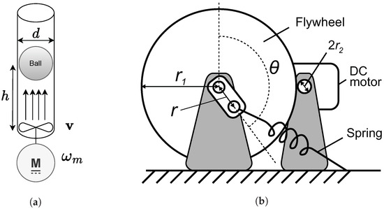
Figure 1. Proposed teaching sets. (a) Ball levitation within a wind tunnel; (b) spring mechanism with a periodic but non-linear load.

2.1. Teaching Set 1: Levitation of a Lightweight Ball

The first teaching set involved the application of levitation control on a lightweight ball using a PID algorithm implemented on an FPGA. The teaching set consisted of three major components: (1) a vertical cylindrical tube with controlled airflow generated at its base; (2) a lightweight ping-pong ball of mass $m\left[\mathrm{kg}\right]$ and diameter $d\left[\mathrm{m}\right]$; and (3) a DC motor-driven propeller responsible for generating the airflow, characterized by motor voltage $V_m$, current $I_m$, resistance $R_m$, and inductance $L_m$. The generated lift force $F_L$ was a function of the airflow velocity v and the aerodynamic properties of the ball. The PID controller processed the ball’s position feedback, adjusting the motor input to maintain the desired levitation height.

2.1.1. Understanding the Underlying Physics and Mathematical Model

To describe the underlying physics of the system, we applied Newton’s second law to model the ball’s vertical motion. The lift force, generated by the airflow from the motor-driven propeller, acted in the upward direction, counteracting the forces pulling the ball downward. These opposing forces included the gravitational force, which was proportional to the ball’s mass, and the aerodynamic drag force, which depended on the ball’s velocity as it moved through the air.

The underlying physics was symbolized using mathematical notation by defining the vertical position of the ball $h\left(t\right)$, the lift force $F_L\left(t\right)$, and the drag force $F_D\left(t\right)$, as indicated in Equation (1),

$$\begin{array}{c}\hfill m{\displaystyle \frac{d^{2}h}{d{t}^2}}={\displaystyle \frac{1}{2}}{C}_L\rho A{(k·{\omega }_m)}^2-mg-{\displaystyle \frac{1}{2}}{C}_D\rho A{\left({\displaystyle \frac{dh}{dt}}\right)}^2,\end{array}$$

(1)

where $C_L$ and $C_D$ were the lift and drag coefficients, respectively; $\rho$ was the air density; A was the cross-sectional area of the ball; g was the gravitational acceleration; and $k·{\omega }_m$ represented a simplified model of the airflow velocity. Although this linear relationship offered a straightforward approach for modeling purposes, it is important to note that the actual relationship can be more complex. In reality, the airflow velocity generated by a propeller depended on several factors, including the design, position, and operating conditions of the propeller. Still, the assumption worked well for the basic analysis and initial controller design, although it is not exact for the general case. At higher speeds or in unusual conditions, real airflow may behave differently due to nonlinear effects [18]. This means that the controller might not perform exactly as predicted if the system moves far from the normal operating range. For more precise control, a more detailed model or adaptive methods would be needed.

In our control system, the goal was to obtain a steady-state condition. To determine it, we considered the scenario in which the ball reached a stable height, which means that its velocity and acceleration were zero. Setting ${\displaystyle \frac{dh}{dt}}=0$ and ${\displaystyle \frac{d^{2}h}{d{t}^2}}=0$, Equation (1) simplifies to Equation (2),

$$0={\displaystyle \frac{1}{2}}{C}_L\rho A{v}^2-mg,$$

(2)

which can be rearranged to solve for the required airflow velocity (Equation (3)):

$$v=\sqrt{{\displaystyle \frac{2mg}{C_L\rho A}}}.$$

(3)

Since the lift coefficient $C_L$ depends on the height h, we can express the airflow velocity required to achieve the desired height with Equation (4)

$$v\left(h\right)=\sqrt{{\displaystyle \frac{2mg}{C_L\left(h\right)\rho A}}}.$$

(4)

This equation provides a relationship between the velocity of airflow and the height of the ball, which was essential to designing the control system to maintain the ball in a desired position.

To determine the required motor speed in revolutions per minute (RPM) to achieve the necessary airflow velocity, we used the following relation:

$$v=k·{\omega }_m,$$

(5)

where ${\omega }_m$ is the angular velocity of the motor in rad/s and k is the proportionality constant relating the motor speed to the airflow velocity. The RPM is given by

$$\mathrm{RPM}={\displaystyle \frac{{\omega }_m}{2\pi }}·60.$$

(6)

Substituting ${\omega }_m=v/k$ into the above equation, we obtained

$$\mathrm{RPM}\left(h\right)={\displaystyle \frac{1}{2\pi }}·60·{\displaystyle \frac{\sqrt{2mg}}{k\sqrt{C_L\left(h\right)\rho A}}}.$$

(7)

This equation determines the required RPM to generate the air flow necessary to maintain the ball at the desired height.

2.1.2. Hardware

For measuring the distance of the ball, the Sharp infrared distance sensor GP2Y0A21YK0F (Sharp Corporation, Osaka, Japan) was used. This sensor reliably measures distances between 10 cm and 80 cm, making it suitable for tracking the ball’s position in real time.

The propulsion system consisted of a 9.6 V DC motor, manufactured by an unbranded company from China. Attached to the motor was a custom 3D-printed propeller, designed to generate airflow. To reduce turbulence and achieve a more laminar flow, a diffuser was installed in front of the propeller.

Electrical hardware included two custom-designed printed circuit boards (PCBs). The first PCB served as a driver circuit for the DC motor. It was a simple design composed of a few discrete components and operated on the basis of rapid switching events controlled by varying duty cycles. These duty cycles were calculated using a control algorithm implemented in a DE0-Nano FPGA Development and Education Kit (Terasic Inc., Hsinchu, Taiwan; Intel Corporation, Santa Clara, CA, USA). This development board used an FPGA as its core, requiring all logic to be implemented in hardware description language (HDL).

The second PCB was designed to interface directly with the DE0-Nano board, providing all necessary connections to the user interface, which was conveniently integrated on the same PCB. The interface included three 7-segment displays that showed individual values of the Kp, Ki, and Kd parameters of the PID controller. In addition, buttons were provided to allow the user to adjust these parameters and observe their effect on system dynamics. A separate display and two buttons enabled the user to modify the reference value.

Figure 2 shows the built wind tunnel, the positioning of the infrared sensor, and the underlying PCB. Buttons for PID control parameters and setpoints were added for ease of tuning. The entire system was powered by a 12 V DC adapter, and all required voltage levels were derived using integrated circuit voltage regulators.

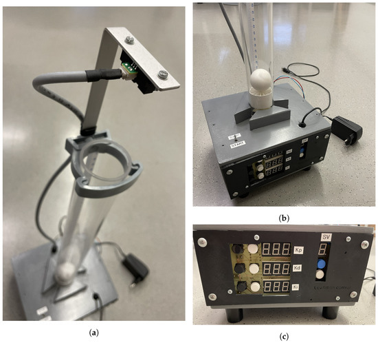
Figure 2. Figures of the wind tunnel. The sensor was intentionally placed 10 cm above the top dead center of the ball, due to sensitivity limitations below this height. A single 12 V DC adapter powered the complete electronics. The user interface allowed changing the $K_p$, $K_i$ and $K_d$ control parameters and the setpoint, denoted as $SV$. (a) Wind tunnel and the sensor; (b) the ground station; and (c) the PCB and user interface.

2.2. Teaching Set 2: Applying the Fuzzy Logic for 1-DOF Spring Mechanism

The second teaching set involved the application of a velocity control on a simple 1-DOF spring mechanism using the AI method (a fuzzy inference logic controller). The traditional PI controller remained implemented as a reference. The teaching set consisted of three major pieces as follows: (1) a spring with a spring constant $k[\mathrm{N}/\mathrm{m}]$ and length $l\left[\mathrm{m}\right]$; (2) an inertia flywheel $J_f\left[{\mathrm{kgm}}^2\right]$ and damping coefficient $B_f\left[\mathrm{Nms}\right]$; and (3) a DC brush electromechanical converter (DC motor) of rotor inertia $J_m\left[{\mathrm{kgm}}^2\right]$, damping coefficient $B_m\left[\mathrm{Nms}\right]$, resistance R and inductance L, and torque and electric constants $K_T,K_E$. A friction drive was utilized to transmit the torque from a motor to the flywheel, where the radius of the DC motor axle, given by $r_1$, and the radius of the flywheel, given by $r_2$, defined the gearing ratio. A reductive gearing ratio, that is, $i={\displaystyle \frac{r_2}{r_1}}<1$, was implemented. Figure 1 represents the sketch of the teaching set.

2.2.1. Understanding the Underlying Physics and Pertaining Mathematical Model

The underlying physics was symbolized using mathematical notation by defining the spring displacement $x_s\left(t\right)$, force $F_s\left(t\right)$, and spring torque ${\tau }_s\left(t\right)$, as denoted in Equation (8),

$$\begin{array}{c}\hfill x_s\left(t\right)=r·\cos \left(\theta \left(t\right)\right)+x_0,\\ \hfill F_s\left(t\right)=k·x_s\left(t\right),\\ \hfill {\tau }_s\left(t\right)=r·F_s\left(t\right)=r·k·[r·\cos \left(\theta \left(t\right)\right)+x_0],\end{array}$$

(8)

where $x_0$ represents the initial displacement in length (m) and r represents the radius of the excenter of the attachment point where the spring was connected to the flywheel to ensure no negative displacement (compression) of the spring.

Motor torque and flywheel dynamics are modeled as effective inertia, comprising (1) inherent inertia of the DC motor (2) and inertia of the flywheel, as described in Equation (9).

$$J=J_m+{\displaystyle \frac{J_f}{i^2}},$$

(9)

where $J_m$ and $J_f$ represent the inertia of the motor and the flywheel, respectively. The motor velocity is denoted by ${\omega }_m$ and the velocity of the flywheel by ${\omega }_f$. Then, the following Equation (10) is stated without accounting for the spring mechanism,

$$J·{\displaystyle \frac{d{\omega }_m\left(t\right)}{dt}}={\tau }_m\left(t\right)-{\displaystyle \frac{{\tau }_f\left(t\right)}{i}}-B_m·{\omega }_m\left(t\right)-B_f·{\omega }_f\left(t\right)-{\tau }_s\left(t\right),$$

(10)

where ${\omega }_m$ represents the motor velocity in radians per second and ${\tau }_m$ represents the motor torque generated. The flywheel torque is denoted as ${\tau }_f={\eta }_g·i·K_T·I\left(t\right)$, where ${\eta }_g$ represents the efficiency of the gear. The teaching set is shown in Figure 3.

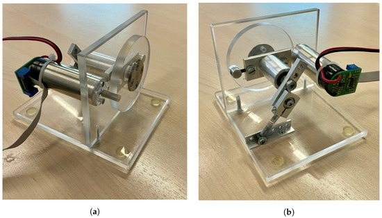
Figure 3. Front and rear views of the spring mechanism, the DC motor, flywheel and transparent structure. (a) Spring mechanism, front view; (b) Spring mechanism, back view.

2.2.2. Fuzzy Logic Controller Implementation on the FPGA

The FLC was implemented in the Intel Quartus II 13.1 environment, which consists of three consecutive steps: (1) fuzzification of the natural input sets into fuzzy sets, (2) fuzzy inference, and (3) defuzzification of fuzzy sets back into naturals. Defuzzification came with the challenge of computing the natural sets from fuzzy sets. Fixed-point division by bit shifting was employed to avoid floating-point division latencies.

The teaching benefits of applying fuzzy logic to the FPGA lie in (1) practicing implementation of the FLC based on the underlying pseudocode that is given in Algorithm 1, (2) practicing FPGA configuration debugging, and (3) practicing the SPI communication protocol from scratch for PC data transfer. Membership functions were defined as signed registers. Figure 4 shows input membership functions, which were defined as triangular, due to the ease of implementation. Derivable functions, such as Gauss or bell, could also have been implemented on the FPGA, but floating-point processing would have been needed. The ranges of membership functions were tuned experimentally. Six sets of membership functions $\mathbf{x}$ were defined, of which three were for negative errors ${\mathbf{x}}_N=\{N^{+},N,N^{-}\}$ and three were for positive errors ${\mathbf{x}}_P=\{P^{-},P,P^{+}\}$. Then, arithmetic averages (midpoints $mid$) were calculated for each membership function. Instead of division by 2, the arithmetic bit to the right for 1 bit was used. The degrees of membership for the fuzzy sets $\mu \left(N^{+}\right)$ and $\mu \left(P^{+}\right)$, that is, the extremes, were calculated as outlined in Equations (11) and (12).

$${\mu }_i\left(N^{+}\right)=\left\{\begin{array}{cc}\left[N_{max}^{+}-e\left[k\right]\right]>>>2\hfill & \mathrm{if}{N}_{min}^{+}\le e\left[k\right]\le N_{max}^{+},\hfill \\ 0\hfill & otherwise,\hfill \end{array}\right.$$

(11)

$${\mu }_i\left(P^{+}\right)=\left\{\begin{array}{cc}\left[e\left[k\right]-P_{min}^{+}\right]>>>2\hfill & \mathrm{if}{P}_{min}^{+}\le e\left[k\right]\le P_{max}^{+},\hfill \\ 0\hfill & otherwise,\hfill \end{array}\right.$$

(12)

Algorithm 1 Fuzzy Logic Control System

1:   Input: control error $e\left[k\right]$ 2:   Output: Control output y 3:   Initialize membership functions (endpoints $min$ and $max$) for velocity input errors $e\left[k\right]$. 4:   Calculate midpoints $mid$ of membership functions. 5:   Calculate degrees of input membership functions ${\mu }_i\left(e\left[k\right]\right)$. 6:   for each fuzzy rule $R_i$ in the rule base do 7:       Compute rule activation strength ${\alpha }_i$ using logical operators (e.g., min/max for AND/OR). 8:       Determine fuzzy output set ${\mu }_o$ based on rule consequence. 9:   end for 10: Combine all fuzzy output sets using a union operation. 11: Compute natural output y using a defuzzification method. 12: return y

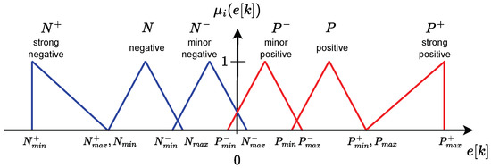
Figure 4. Input velocity error triangular membership functions. Blue = negative velocity error membership functions, $N^{-},N,N^{+}$. Red = positive velocity error membership functions, $P^{-},P,P^{+}$.

The membership functions $\mu (N),\mu (P)$ are calculated as described in Equation (13). Similarly, the membership functions for $\mu (N^{-}),\mu \left(P^{-}\right)$ are calculated.

$$\begin{array}{c}\hfill {\mu }_{i,A}\left(N\right)=\left\{\begin{array}{cc}\left[e\left[k\right]-N_{min}\right]>>>1\hfill & \mathrm{if}{N}_{min}\le e\left[k\right]<N_{mid},\hfill \\ 0\hfill & otherwise,\hfill \end{array}\right.\\ \hfill {\mu }_{i,B}\left(N\right)=\left\{\begin{array}{cc}\left[N_{max}-e\left[k\right]\right]>>>1\hfill & \mathrm{if}{N}_{mid}\le e\left[k\right]\le N_{max},\hfill \\ 0\hfill & otherwise,\hfill \end{array}\right.\\ \hfill {\mu }_{i,A}\left(P\right)=\left\{\begin{array}{cc}\left[e\left[k\right]-P_{min}\right]>>>1\hfill & \mathrm{if}{P}_{min}\le e\left[k\right]<P_{mid},\hfill \\ 0\hfill & otherwise,\hfill \end{array}\right.\\ \hfill {\mu }_{i,B}\left(P\right)=\left\{\begin{array}{cc}\left[P_{max}-e\left[k\right]\right]>>>1\hfill & \mathrm{if}{P}_{mid}\le e\left[k\right]\le P_{max},\hfill \\ 0\hfill & otherwise,\hfill \end{array}\right.\end{array}$$

(13)

where A represents the area where $min\le e\left[k\right]<mid$ and B represents the area where $mid\le e\left[k\right]\le max$. Finally, fuzzification for intermediate membership functions was concluded by summing the A and B signals as follows:

$$\begin{array}{c}\hfill {\mu }_i\left(N\right)={\mu }_{i,A}\left(N\right)+{\mu }_{i,B}\left(N\right),\\ \hfill {\mu }_i\left(P\right)={\mu }_{i,A}\left(P\right)+{\mu }_{i,B}\left(P\right),\\ \hfill {\mu }_i\left(N^{-}\right)={\mu }_{i,A}\left(N^{-}\right)+{\mu }_{i,B}\left(N^{-}\right),\\ \hfill {\mu }_i\left(P^{-}\right)={\mu }_{i,A}\left(P^{-}\right)+{\mu }_{i,B}\left(P^{-}\right).\end{array}$$

(14)

Fuzzy inference was performed using the if-then rule database. The database consisted of the following six rules:

• If velocity error $e\left[k\right]$ strong negative $N^{+}$ then accelerate heavily $A^{+}$;
• If velocity error $e\left[k\right]$ negative N then accelerate A;
• If velocity error $e\left[k\right]$ minor negative $N^{-}$ then accelerate slightly $A^{-}$;
• If velocity error $e\left[k\right]$ slightly positive $P^{-}$ then decelerate slightly $D^{-}$;
• If velocity error $e\left[k\right]$ positive P then decelerate D;
• If velocity error $e\left[k\right]$ strong positive $P^{+}$ then decelerate heavily $D^{+}$.

Defuzzification was performed using output membership singletons. There are seven different singletons implemented, which are depicted in Figure 5. Output singletons were used for ease of understanding and quick adaptation. Here, the parameters of the x-axis $u_f$ were tuned. Again, the positions of singletons were tuned experimentally, where their positioning denoted the underlying motor power (the PWM control signal). Positioning black, green, and blue singletons away from the central M increased the underlying motor power and thus reduced the time delays. Positioning them closer to M reduced motor power and increased time delays. The trade-off was necessary. A moving average finite impulse filter with a time window of four samples allowed applying a smoother control value u.

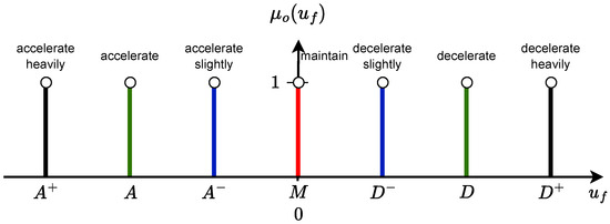
Figure 5. The output membership singletons. Three are negatives, three are positives, and one is neutral. Black = accelerate and decelerate heavily, $A^{+},D^{+}$. Green = accelerate and decelerate normally, $A,D$. Blue = accelerate and decelerate slightly, $A^{-},D^{-}$. Red = maintain, M.

2.2.3. Practical Implementation of the Fuzzy Logic on the FPGA

The practical implementation of the FLC included the acquisition of input data, processing, and setting the output value. Acquisition of input data included ADC readings with I2C communication and reading the DC motor velocity. Processing included calculating the output value, which was then converted through a digital-to-analog (DAC) conversion using pulse width modulation (PWM). For easier understanding of a flow of signals, a common notation and a bit width of a signal were established, as shown in Table 1.

Table 1. Name of the signals (variable), bit width, and visualization.

Signal	Bit Width	Visualization
$CLK$	1 bit	1’b x
$Co{m}_{CLK}$	1 bit	1’b x
$iCLK$	1 bit	1’b x
$CNT$	8 bit	8’b xxxx.xxxx
$CMP$	8 bit	8’b xxxx.xxxx
$oRST$	1 bit	1’b x
$T_v$	1 bit	1’b x
$EN$	1 bit	1’b x
$CS$	1 bit	1’b x
$oEND$	1 bit	1’b x
$oI2C$	12 bit	12’b xxxx.xxxx.xxxx
$error$	16 bit	16’b s1xxx.xxxx.xxxx.xxxx
u	9 bit	9’b sxxxx.xxxx
$DIR$	1 bit	1’b x
$oDR1$	7 bit	7’b xxx.xxxx
$oDR2$	7 bit	7’b xxx.xxxx

The input clock $CLK$ for the FPGA operation came from the internal FPGA clock. As the frequency of $CLK=50$ MHz, two different phased-locked loop (PLL) prescalers were created for down-sizing: (1) a prescaler with a ratio of $PL{L}_1=1/16$ to power the PWM clock of frequency $iCLK=3.125$ MHz and (2) a prescaler with a ratio $PL{L}_2=1/8$ to power the I2C communication of frequency $Co{m}_{CLK}=6.25$ MHz. There $iCLK$ was an input into the PWM block, an 8-bit counter $CNT$ value that counted from 0 to 255 and then subtracted from 255 back to 0 to symbolize a rectified symmetric triangular form of the signal. The PWM block provided two additional synchronization outputs, i.e., $oRST$, which was set to 1 exactly when $CNT=255$ and reset otherwise, and $T_v$, which was set to 1 exactly when $CNT=0$ and reset otherwise. The first acted as an interruption for current AD conversion, that is, current sampling time $T_i=20$ kHz, the second as an interruption to execute the velocity feedback loop and calculate the new duty rate (PWM width), that is, velocity sampling time $T_v=200$ Hz. Two comparison values, $CM{P}_1$ and $CM{P}_2$, were constantly checked for the statement $CMP<CNT$ to drive the DC motor with a given duty rate $oDR1$ and $oDR2$; if true, then the output was set to 1 (the power transistor set to on), if false, then the output was set to 0. The $oDR1$ ran the DC motor in the positive direction and the $oDR2$ in the negative direction, where $DIR$ stated the direction of rotation.

The signals for I2C communication between the FPGA and the ADC module included the enable signal $EN$, the chip select signal $CS$, the channel $iCH$, the synchronization signal for the end of the conversion $oEND$, and the result signal where the result of the conversion was written in $oI2C$. The I2C communication ran at a frequency $Co{m}_{CLK}=6.25$ MHz, which was higher than recommended. However, no loss of information was noticed, even when running at that frequency.

The signals for reading the velocity of the DC motor included the input clock $iCLK$. Two different signals came from the incremental encoder, $A_{inc}$ and $B_{inc}$. The shift between the two gave information on the direction of a rotation. The rate of change gave information about the DC motor’s velocity.

The DC motor control sketch is depicted in Figure 6. There were two feedback loops, the internal current control loop and the external velocity control loop. The internal current loop was PI-controlled. The external velocity loop was controlled either by a PI controller or by the FLC.

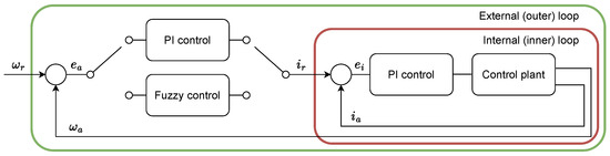
Figure 6. Cascade current and velocity control. PI current control and selectable PI vs. fuzzy velocity control. ${\omega }_r$= reference velocity, ${\omega }_a$ = actual velocity, $e_a$ = velocity control error. $i_r$ = reference current, $i_a$ = actual current, $e_i$ = current control error. Control plant = DC mechanism.

3. Experiments and Results

To demonstrate the functioning of the algorithms implemented, several experiments were performed. Each experiment allowed for arbitrarily setting the control constants to observe the effect. The objective of ball levitation was to hold the ball at the desired height given $h_r$. Therefore, a position control was implemented for it, where the angular frequency of the DC motor was used as a control signal u. The objective of the spring mechanism was to implement a control of the velocity. The goal was to maintain a constant rotational speed of the DC motor, despite the external disturbances caused by the attached spring.

The goodness of control was monitored by setting the desired setpoints, typically using a step function, and evaluating the step response of the system. Overshooting, steady-state error, and lagged response are all factors that decrease overall goodness of control but are inherent parts of the wrongly set control constants.

3.1. Experimental Setup

The Terasic DE0-Nano FPGA was used for the practical implementation of both teaching sets. The Quartus II programming environment with the Verilog configuration language was used. For the FLC, input triangular membership functions and output singletons were set as outlined in Table 2.

Table 2. Parameter settings on input membership functions and output singletons.

Input Triangular Membership Functions			Output Singletons
Function Name	Min	Max	Singleton	Value
$N^{+}$	$-2096$	$-512$	${\mu }_f\left(A^{+}\right)$	$-75$
N	$-512$	$-32$	${\mu }_f\left(A\right)$	$-55$
$N^{-}$	$-56$	16	${\mu }_f\left(A^{-}\right)$	$-10$
$P^{-}$	$-16$	56	${\mu }_f\left(M\right)$	0
P	32	512	${\mu }_f\left(D^{-}\right)$	10
$P^{+}$	512	2096	${\mu }_f\left(D\right)$	55
			${\mu }_f\left(D^{+}\right)$	75

3.2. Evaluation Criteria

Teaching sets are an excellent didactic tool for (1) observing the behavior of the systems when being controlled in a feedback loop, (2) learning the evaluation criteria of the goodness of feedback control, (3) and seeing the effect and tuning of controller parameters. The Heaviside step function was used for excitation, since it is among the more common techniques for exciting the system, where the system undergoes a step response. Some common evaluation criteria that are to be studied with step responses involve overshoot A, rise time $t_r$, steady-state error $e_{ss}$, and settle time $t_{sett}$. For tuning and optimization of control parameters, the mean squared error $\left(mse\right)$ is common. For the non-linear spring mechanism, the standard deviation of the oscillation $std\_osc$ is also a reasonable indicator.

3.3. Results

The reference value of velocity ${\omega }_r$ (also called a set point, depicted as a dotted black line) of the 1-DOF control mechanism had been changing between minimum and maximum velocity values, ${\omega }_{min}=-600$ quants per sample time $t_s$ and ${\omega }_{max}=600$ quants per sample time $t_s$. The actual velocity value ${\omega }_a$ (also called the process variable, depicted as a red line) followed the reference velocity value ${\omega }_r$ to a better or worse degree. The control signal (the controller output, depicted as a blue line) was also visualized.

3.3.1. Results on Ball Levitation

The experiments for set 1 of the teaching involved positioning the ball height within the wind tunnel. Nine different reference positions $h_r$ were tested, which are shown by black dotted lines in Figure 7. The red line was visualized to represent the actual height $h_a$. Figure 8 was attached to represent the functioning of the PID control on the larger time scale.

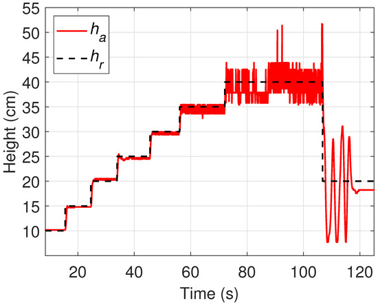
Figure 7. Results for ball levitation within the wind tunnel with PI control. As the ball approached the distance sensor (reference height $h_r=40$ cm), the sensitivity of the sensor was increased and oscillations arose.

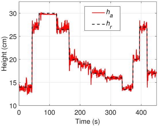
Figure 8. Results for ball levitation within the wind tunnel, with dynamic changes of reference value over a larger time scale. The standard deviation of the signal was larger for higher reference values $h_r$ and smaller for lower values.

The PID performance for the first part was solid, the dynamics in small incremental reference changes were rapid, and minimal overshoots were indicated. The steady-state error was easily eliminated. By increasing the height, the ball physically approached the sensor, which increased its sensitivity. Hence, significant oscillations appeared. Significant overshoots were also exhibited by incremental reference changes. Further fine-tuning of the control parameters to eliminate the steady-state error for such scenarios and reduce the level of overshoot is necessary.

3.3.2. Results on Spring Mechanism

The results on the spring mechanism were obtained first using the velocity PI control as a benchmark. The FLC was then tested. For the proof of concept, a single run was performed, where significant oscillations were observed for both controllers due to the non-linear load imposed by the spring. The test was then repeated 10 consecutive times ($n=10$) to observe statistical differences between the two controllers. The reference and actual velocities and the control error, that is, $e\left[k\right]={\omega }_r\left[k\right]-{\omega }_a\left[k\right]$, were monitored. Then, the mean squared error $mse=\mathbb{E}\left[{({\omega }_r-{\omega }_a)}^2\right]$ was calculated.

Figure 9 and Figure 10 represent the step responses of the PID and FLC controllers. As shown viaully, the PID scored a lower amplitude of oscillations but a higher chattering of the control value u. The FLC suffered from chattering when ${\omega }_r=0$. Steady-state error was eliminated well for both controllers.

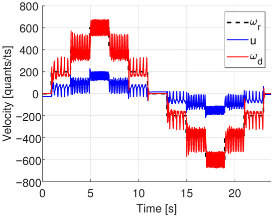
Figure 9. The PI performance on the non-linear spring mechanism. Steady-state error was eliminated, but large oscillations were still present.

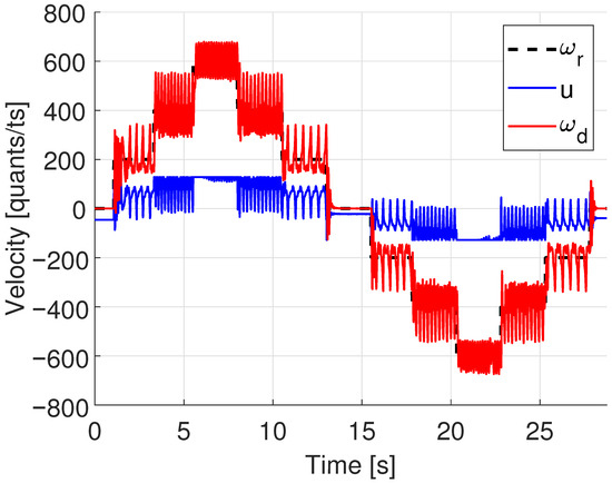
Figure 10. The FLC performance on the non-linear spring mechanism. An I controller was connected in series with a fuzzy controller for improved steady-state tracking. Chattering close to ${\omega }_r=0$ was present.

The plain-vanilla FLC underwent a steady-state error. Therefore, an I controller was wired in series with the FLC. The results of the statistical analysis to compare the PI (reference) and FLC controller algorithms are shown in the second and third columns of Table 3. The standard deviations of the control error $stdev\left(e\right[k\left]\right)$ (oscillations) were also calculated and are visualized in the fourth and fifth columns of Table 3.

Table 3. The statistical analysis of the mean values and standard deviations (stdev) of the oscillations, $n=10$. The PI acted as a benchmark and worked better than the FLC. Additional tuning of the FLC is necessary.

	Mean Error $\mathbb{E}\left({\mathit{mse}}_{\mathit{i}}\right)$		Stdev of Oscillations $\mathit{stdev}\left({\mathit{mse}}_{\mathit{i}}\right)$
Run	PI	FLC	PI	FLC
1	3829.18	4203.14	61.89	64.85
2	3652.21	4063.60	60.45	63.76
3	3706.62	4106.59	60.89	64.10
4	3870.04	4215.86	62.22	64.94
5	3918.14	4184.71	62.61	64.70
6	3855.74	4367.55	62.11	66.10
7	3864.81	4143.20	62.18	64.38
8	3864.20	4077.71	62.18	63.87
9	3865.01	4114.42	62.18	64.16
10	3870.59	4258.95	62.35	62.58
mean	3829.65	4173.57	61.91	64.34
std	83.08	93.03	0.68	0.92
min	3652.21	4063.60	60.45	62.58
max	3918.14	4367.55	62.61	66.10

The interpretation of the results shows that the PI performed better than the FLC with regard to both the mean error of $ms{e}_i$, that is, $\mathbb{E}\left(ms{e}_i\right)$, and the standard deviations of the oscillations $std\_osc=stdev\left(ms{e}_i\right)$, where $i=1,2,\dots ,10$. This was indicated by lower mean errors and a lower amplitude of oscillations. Further tuning of membership functions and singletons is necessary. The improvement in the amplitude of the oscillations could be enhanced by adding the D controller for the PID or by integrating another set of inputs, the acceleration, for the FLC. In this way, the acceleration input could mimic the D controller for extra damping close to the reference point. There is a potential for future FLC tuning improvements.

3.3.3. Discussion

The proposed teaching sets were compared with several related references noted in the Introduction. Aguilera-Alvarez et al. [2] presented a virtual didactic tool implemented entirely in a simulation environment. Although their work focused on improving students’ understanding of membership functions, fuzzy rules, and defuzzification—objectives similar to ours—the lack of real-world implementation represents a limitation compared to our study. Their main benefit was the statistical assessment of student learning through a perception survey comparing LabView and MATLAB users. In contrast, our contribution included a practical case study, although without formal knowledge evaluation, and additionally integrated FPGA hardware, which their approach did not.

Barbosa et al. [3] incorporated FPGA hardware but used an FPGA-in-the-loop setup to drive an induction motor under scalar control. This task was less challenging than driving a non-linear system. Moreover, the authors did not clarify whether the motor operated under load. Their approach relied on a simulated motor model rather than a fully implemented real-world application. No assessment of learning outcomes related to FPGA programming or fuzzy logic control (FLC) was provided.

Artal-Sevil et al. [4] demonstrated a magnetic ball levitation system, which was inherently more demanding than the ping-pong ball used in our work due to faster dynamics and system instability. Their control structure used both current and position loops, whereas in our study, the current loop was applied only to handle non-linear behavior. They employed a Hall sensor instead of an infrared one and successfully proved the concept. However, they did not benchmark against alternatives such as PID control, nor did they use FPGA hardware. The contribution focused on demonstration rather than comprehensive didactic evaluation. As the application remained largely simulation-based, its educational impact on understanding FLCs and nonlinear control was limited.

Alba-Flores et al. [5] presented a semester-long laboratory exercise involving autonomous mobile robots, a significantly more complex topic than our proposed setups. Student teams implemented PID, FLC, and ANN controllers, first in simulation and then on FPGAs embedded in robots. Their rigorous assessment reported strong learning outcomes.

Abdelmoula et al. [6] used autonomous mobile robots in a similar way, aiming to familiarize students with DC and stepper motor drives and other components. The implemented tasks, such as navigation, path planning, and autonomous parking, were all more complex than our applications. However, the paper emphasized system integration rather than detailed didactic assessment or learning benefits.

Cervantez et al. [7] proposed a practical tool for teaching buck converter control. Although relevant, this application differed fundamentally from levitation and nonlinear spring control, as it focused solely on current regulation. The FPGA configuration was performed through LabView, and only a limited discussion was provided on didactic outcomes. However, the authors indicated that the platform could have enhanced students’ understanding.

4. Conclusions

Two different didactic teaching sets for students of a class on intelligent control techniques in mechatronics have been developed and tested. Both teaching sets allowed for the implementation of custom control algorithms and allowed for live tuning of control parameters. For a proof of concept, the classical PI control algorithm was utilized. For more robust non-linear control, a custom fuzzy controller was implemented.

Using the teaching sets, the underlying physics can be studied first to derive the outlook and structure of the control algorithm. The analog model can then be derived and discretized in a digital form that then run on the FPGA. So far, both the fuzzy and the PI controllers have been implemented using fixed-point representation.

Setting the control parameters interactively live during the operation drastically improved understanding of control theory in practice. Teaching set 1 had physical buttons installed for the PID parameters, while teaching set 2 used a constant input–output UART connection to the PC. Within the control command, the parameters were tuned. In addition, a UART connection was used for the transfer of data variables from the FPGA to the PC, which allowed interactive live plotting.

Further advances include the implementation of controllers using floating-point representation. In addition, automated tuning or hybridization using a nature-inspired optimization algorithm could be employed, such as a genetic algorithm or differential evolution. Last but not least, laboratory exercises could be extended with the Register-Transfer Level (RTL) simulation for a more comprehensive understanding.

References

- Zadeh, L. Fuzzy sets. Inf. Control 1965, 8, 338–353. [Google Scholar] [CrossRef]
- Aguilera-Alvarez, J.; Padilla-Medina, J.; Martínez-Nolasco, C.; Samano-Ortega, V.; Bravo-Sanchez, M.; Martínez-Nolasco, J. Development of a Didactic Educational Tool for Learning Fuzzy Control Systems. Math. Probl. Eng. 2021, 2021, 1–17. [Google Scholar] [CrossRef]
- Barbosa, R.; Pelzl, M.; Cordero, R.; Caramalac, M.; Suemitsu, W. Didactic FPGA-in-the-Loop Scalar Fuzzy Control Setup for Motor Drive Education. In Proceedings of the 2023 IEEE 8th Southern Power Electronics Conference and 17th Brazilian Power Electronics Conference (SPEC/COBEP), Florianopolis, Brazil, 26–29 November 2023; pp. 1–5. [Google Scholar] [CrossRef]
- Artal-Sevil, J.; Bernal-Ruiz, C.; Bono-Nuez, A.; Penas, M.S. Design of a Fuzzy-Controller for a Magnetic Levitation System using Hall-Effect sensors. In Proceedings of the 2020 XIV Technologies Applied to Electronics Teaching Conference (TAEE), Porto, Portugal, 8–10 July 2020; pp. 1–9. [Google Scholar] [CrossRef]
- Alba-Flores, R.; Rios-Gutierrez, F. Control Systems Design Course with a Focus for Applications in Mobile Robotics. In Proceedings of the 2013 ASEE Annual Conference & Exposition Proceedings, Atlanta, GA, USA, 23–26 June 2013; pp. 23.338.1–23.338.13. [Google Scholar] [CrossRef]
- Abdelmoula, C.; Chaari, F.; Masmoudi, M. Real time algorithm implemented in Altera’s FPGA for a newly designed mobile robot. Multidiscip. Model. Mater. Struct. 2014, 10, 75–93. [Google Scholar] [CrossRef]
- Cervantes, M.H.; Ramirez, M.C.G.; Gomez, J.C.; Anguiano, A.C.T.; Cardenas, F.M. Real-time simulation of a buck converter for educational purposes in a LabView-programmed FPGA. In Proceedings of the 2014 IEEE International Autumn Meeting on Power, Electronics and Computing (ROPEC), Ixtapa, Mexico, 5–7 November 2014; pp. 1–6. [Google Scholar] [CrossRef]
- Seng, K.P.; Lee, P.J.; Ang, L.M. Embedded Intelligence on FPGA: Survey, Applications and Challenges. Electronics 2021, 10, 895. [Google Scholar] [CrossRef]
- Hermassi, M.; Krim, S.; Kraiem, Y.; Hajjaji, M.A. Adaptive neuro fuzzy technology to enhance PID performances within VCA for grid-connected wind system under nonlinear behaviors: FPGA hardware implementation. Comput. Electr. Eng. 2024, 117, 109264. [Google Scholar] [CrossRef]
- Swami, R.K.; Kumar, V.; Joshi, R.R. FPGA-based Implementation of Fuzzy Logic DTC for Induction Motor Drive Fed by Matrix Converter. IETE J. Res. 2022, 68, 1418–1426. [Google Scholar] [CrossRef]
- Deliparaschos, K.M.; Nenedakis, F.I.; Tzafestas, S.G. Design and Implementation of a Fast Digital Fuzzy Logic Controller Using FPGA Technology. J. Intell. Robot. Syst. 2006, 45, 77–96. [Google Scholar] [CrossRef]
- Akbatı, O.; Üzgün, H.D.; Akkaya, S. Hardware-in-the-loop simulation and implementation of a fuzzy logic controller with FPGA: Case study of a magnetic levitation system. Trans. Inst. Meas. Control 2019, 41, 2150–2159. [Google Scholar] [CrossRef]
- Silva, S.N.; Lopes, F.F.; Valderrama, C.; Fernandes, M.A.C. Proposal of Takagi–Sugeno Fuzzy-PI Controller Hardware. Sensors 2020, 20, 1996. [Google Scholar] [CrossRef] [PubMed]
- Jhang, J.Y.; Tang, K.H.; Huang, C.K.; Lin, C.J.; Young, K.Y. FPGA Implementation of a Functional Neuro-Fuzzy Network for Nonlinear System Control. Electronics 2018, 7, 145. [Google Scholar] [CrossRef]
- Ahmed, S.; Yahia, K. Implementation of Fuzzy Logic Controller Algorithms with MF optimization on FPGA. Stat. Optim. Inf. Comput. 2024, 12, 182–199. [Google Scholar] [CrossRef]
- Bernal, E.; Lagunes, M.L.; Castillo, O.; Soria, J.; Valdez, F. Optimization of Type-2 Fuzzy Logic Controller Design Using the GSO and FA Algorithms. Int. J. Fuzzy Syst. 2021, 23, 42–57. [Google Scholar] [CrossRef]
- Varshney, A.; Goyal, V. Re-evaluation on fuzzy logic controlled system by optimizing the membership functions. Mater. Today Proc. 2023. [Google Scholar] [CrossRef]
- Tkáčik, T.; Tkáčik, M.; Jadlovská, S.; Jadlovská, A. Design of Aerodynamic Ball Levitation Laboratory Plant. Processes 2021, 9, 1950. [Google Scholar] [CrossRef]
Disclaimer/Publisher’s Note: The statements, opinions and data contained in all publications are solely those of the individual author(s) and contributor(s) and not of MDPI and/or the editor(s). MDPI and/or the editor(s) disclaim responsibility for any injury to people or property resulting from any ideas, methods, instructions or products referred to in the content. |
© 2025 by the authors. Licensee MDPI, Basel, Switzerland. This article is an open access article distributed under the terms and conditions of the Creative Commons Attribution (CC BY) license (https://creativecommons.org/licenses/by/4.0/).