Impact of LED Light Spatial Distribution on Photosynthetic Radiation Uniformity in Indoor Crops

Abstract

The integration of LED lighting enables precise radiation control in plant factory cultivation systems. While LEDs offer energy efficiency and spectral tuning, achieving a uniform photosynthetic photon flux density (PPFD) remains a critical technical challenge. This study evaluated the impact of three spatial LED configurations on irradiance uniformity using commercial horticultural LEDs and a light recipe of 75% red and 25% blue. Optical simulations in TracePro^® 2017 were conducted to analyze radiant flux, optical efficiency, and uniformity, along with LED quantity, system cost, and electrical consumption under two environmental scenarios: open (without reflective walls) and closed (with reflective walls). Results show that distribution 3, which featured reduced central LED density, achieved 4–8% higher homogeneity in the open scenario, and 2.7–6.5% in the closed scenario, compared to symmetric layouts (distribution 1 and 2). Reflective walls increased average PPFD by up to 20% and optical efficiency by around 9%, with a minimal effect on uniformity. Lowering the lamp-to-canopy distance from 35 cm to 30 cm resulted in a 10% increase in PPFD. Despite a reduction in total photon flux, distribution 3 exhibited superior irradiance homogeneity. One-way ANOVA confirmed significant effects of environment, height, and LED model (p < 0.05), but not of spatial alone. This simulation-based methodology offers a robust framework for optimizing energy-efficient lighting systems. Future work will explore the integrating of non-visible wavelengths and experimental validations to extend practical applicability.

1. Introduction

Light plays a crucial role in the growth and development of plants during their maturation phase, as it is not only their primary source of energy, but it is also acted upon as an environmental signal that regulates essential physiological processes [1]. Photosynthetically active radiation (PAR), ranging between 400 and 700 nm wavelengths, is the spectrum of light most utilized by plants for photosynthesis. Within this range, blue light (B, 400–500 nm) and red light (R, 600–700 nm) are absorbed by the photosynthetic pigments, favoring carbohydrate production and the release of oxygen into the atmosphere [2]. In addition to its role as an energy source, light influences key photomorphogenic responses such as germination, stem elongation, leaf expansion, flowering and the biosynthesis of secondary metabolites [3]. These processes are regulated by photoreceptors such as phytochromes, cryptochromes, and phototropins, which allow plants to detect and respond to changes in the intensity, quality, duration, and direction of light [4].

In recent years, plant factory with artificial lighting (PFAL) systems have emerged as a groundbreaking solution to the pressing challenges facing modern agriculture—ranging from food security and rapid urban expansion to the escalating impacts of climate change [5]. By replacement natural sunlight with artificial light sources, PFAL systems enable precise environmental control, ensuring uninterrupted production regardless external of conditions [6]. Within this context, light-emitting diode (LED) technology has gained prominence due to its superior energy efficiency and its ability to finely tune the spectral quality of light, which can lead to substantial increases in productivity [7,8]. Several recent studies have highlighted the importance of tailored light spectra to enhance crop-specific performance in controlled environments. For instance, Pannico et al. [2] demonstrated improved yield and nutraceutical content in potato crops using targeted red-blue supplementation. However, uneven light distribution remains a critical challenge, as it can cause irregular plant growth, reduced yields, and increased energy consumption [9]. To address these issues, recent efforts have focused on the integration of artificial intelligence approaches that merge environmental and cultivation data to anticipate adverse conditions and enhance decision-making within controlled environments. These methods have shown promising results in the ongoing optimization of PFAL systems [10].

However, one of the main challenges in the implementation of artificial lighting in indoor agriculture is the non-uniform distribution of radiation, which generates variability in plant growth, reduces yields, and increases energy consumption [11].

To address this challenge, various studies have developed optical models that allow the design and evaluation of lighting systems that minimize fluctuations in irradiance. Asiabanpour et al. [12] used AGI32 to simulate a LED lighting system (450–660 nm) with optical fiber in greenhouses, modeling the light distribution and uniformity, achieving 85% simulated uniformity in the irradiance pattern. Similarly, Bo et al. [13] conducted a simulation of solar radiation distribution in a three-span plastic greenhouse. They combined a greenhouse solar radiation model with an optical simulation system to predict light transmission and distribution. The model examined variations in irradiance within the greenhouse structure, evaluating light uniformity and its effectiveness for plant growth. Additionally, Park and Runkle [14] implemented a strategy to achieve uniform far-red radiation distribution (730 nm) using strategically placed LED bars and a controlled photoperiod. However, this strategy may induce excessive stem elongation, compromise the structural stability of plants, and limit its applicability across different crop species.

In vertical farming systems, fluorescent coatings were applied to luminaires by Yalçın and Ertürk [15], resulting in a 20–35% increase in PAR irradiance without increasing energy consumption. However, the effectiveness of this strategy depends on the type of crop, the durability of the coating and the compatibility with the luminaires. Meanwhile, a fiber optic system with Fresnel lenses was optimized by Vu et al. [16] to distribute solar light in indoor crops, achieving 65% efficiency in radiation transmission and improving light uniformity. Nevertheless, the system’s performance is conditioned by solar availability, optical losses and high installation costs. Finally, the arrangement of LEDs in a PFAL system was improved by Lee et al. [17] using 3D ray tracing, resulting in a uniform distribution (18.5% variability, 267.5 µmol m⁻² s⁻¹ intensity) and homogeneous growth in cucumber and watermelon seedlings. However, its application is limited to certain crops and environments, with no evaluation of the energy impact.

On the other hand, in various studies, ray-tracing optical simulations have been employed as a tool to improve the uniformity of LED lighting systems. For example, in the work of J. Mei and J. Zou [18], the irradiance of LED arrays was improved using a particle swarm optimization (PSO) method, with practical constraints such as thermal dissipation and circuit board wiring being considered. Nevertheless, despite achieving a uniformity of 95%, the assessment was restricted to a measurement distance of 3 cm between the emitting and receiving surfaces, and was confined to a target area of only 16 × 16 cm.

For plant growth applications, the influence of the number of emitters and their bidimensional arrangement in a mushroom-incubator-type structure was analyzed by J. Bai et al. [19], with the aim of designing improved LED arrays. Although the resulting LED array increased irradiance uniformity to 97%, the nature of the incubator constituted a small, enclosed space, which differs from the conditions applicable to vertical farming. Finally, in the work of K. Xu et al. [20], a triangular prism was incorporated into the base plate of the array, combining a laser diode with LED illumination; however, although uniformity was increased to 88%, the addition of components to the base of the lamp increased the complexity of its manufacture, which could compromise the practical feasibility of this solution.

Although advances in the simulation of lighting systems for controlled crop environments have improved the design of light sources, current approaches are still lacking a systematic methodology to compare and optimize LED radiation distribution prior to implementation. Critical variables such as spectral dispersion, environmental reflectance, and the interaction between multiple LED sources are often omitted, which limits irradiance uniformity and leads to variations in plant growth and energy consumption. To address this gap, TracePro^®, a widely validated Monte Carlo ray-tracing software [21], is employed in this study to develop a comparison methodology that evaluates the LED radiation distribution in indoor crop systems. Through this approach, the spatial arrangement of light sources is analyzed, and the uniformity of PPFD is improved to avoid crop physiological consequences such as poor growth or light-uneven stress, providing a reliable basis for the design of more efficient lighting systems.

Three different LED distributions will be explored to ensure a PPFD of at least 150 µmol m⁻² s⁻¹ over the entire illuminated area, avoiding any negative impact on plant development and promoting better crop growth, as indicated by Rakutko and Rakutko [22]. To evaluate the homogeneity and uniformity of each distribution with a light recipe, the lamps will be applied in vertical farms at a growth rack level. In this context, the selection of materials, the optical modeling of LEDs, the different spatial distributions, the optical simulation parameters, and the execution of simulations are described in Section 2. In Section 3, comparative results are presented based on total values such as the number of LEDs, overall system cost, and electrical energy consumption, as well as PPFD and uniformity in two reflectance scenarios. Additionally, analyses using irradiance maps, statistical data, and irradiated area are included. Finally, in Section 4 and Section 5, the discussion of results, conclusions and key points of this study are presented.

2. Materials and Methods

2.1. Summary of Procedure

Figure 1 depicts four stages of the methodology for evaluating the spatial distributions of LEDs used in horticulture. This analysis was carried out through simulations under different configuration scenarios, applying a light recipe with an R/B 3:1 ratio (75% red, R + 25% blue, B) based on PPFD percentage. This configuration, widely adopted in horticultural lighting systems, was implemented to evaluate its effect on radiation uniformity (u) and optical efficiency (ηₒ) over the cultivation area [2,9,23]. In the first stage, commercial LEDs with similar characteristics in terms of emission angle and spectral emission were selected based on this same light recipe. Here, the physical dimensions (the area where the simulations were conducted) of the vertical farming structure and the placement of the light sources were established. The second stage involved modeling the light source with the selected LEDs, incorporating manufacturer data and configuring optical elements (reflectors and absorbing surfaces) to simulate under operating conditions. Additionally, the number of emitter devices required to achieve the light recipe was determined considering an efficiency of 30%, which indicates that only one-third of the energy is converted into useful light and directly influences the number of emitters needed to reach the desired radiation levels [22]. The third stage consisted of designing the experiment for the simulations, considering parameters such as LED configuration variables such as LED combinations, spatial distribution, reflective conditions, and the height between the emitters and the receiving area. Finally, based on the results, comparison criteria were selected to evaluate the performance of the different LED configurations.

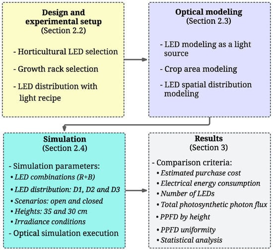
Figure 1. Flowchart of the methodology employed.

2.2. Design and Experimental Setup

2.2.1. Horticultural LED Selection

Commercial monochromatic horticultural LEDs from OSRAM, SAMSUNG, and CREE were selected, all of them recognized as among the top five brands worldwide specializing in plant growth solutions, emitting at wavelengths (λ) red and blue, considering key parameters extracted from their respective data sheets. Table 1 summarizes the evaluated parameters, which include radiant flux (Rflux), photosynthetic photon flux (PPF), emission angle (θ), peak wavelength (λ_peak), forward voltage (V), forward current (I), electrical energy consumption (P), and cost per thousand (USD).

Table 1. Characteristics of monochromatic commercial LED for horticulture of R and B electromagnetic spectrum emission.

LED	Brand	Model	λpeak (nm)	Rflux (mW)	PPF (μmol s−1)	θ (o)	V (V)	I (mA)	P (W)	USD 1000 u
LED 1	OSRAM	GH CSSRM5.24 [24]	660	1068	5.83	120	1.99	700	1.4	0.81
LED 2	SAMSUNG	LH351H 2W [25]	660	1060	5.82	120	2.06	700	1.4	0.665
LED 3	CREE	XP-G3 Photo Red [26]	645	500	2.72	123	1.99	350	0.7	2.72
LED 4	OSRAM	GD CSSRM3.14 [27]	445	1555	5.75	120	2.92	700	2	1.07
LED 5	SAMSUNG	LH351H Blue [28]	450	750	2.8	130	2.86	350	1	0.27
LED 6	CREE	XP-G3 Royal Blue [26]	451	730	2.77	130	2.79	350	1	1.73

Table 1. Characteristics of monochromatic commercial LED for horticulture of R and B electromagnetic spectrum emission.

LED	Brand	Model	λpeak (nm)	Rflux (mW)	PPF (μmol s−1)	θ (o)	V (V)	I (mA)	P (W)	USD 1000 u
LED 1	OSRAM	GH CSSRM5.24 [24]	660	1068	5.83	120	1.99	700	1.4	0.81
LED 2	SAMSUNG	LH351H 2W [25]	660	1060	5.82	120	2.06	700	1.4	0.665
LED 3	CREE	XP-G3 Photo Red [26]	645	500	2.72	123	1.99	350	0.7	2.72
LED 4	OSRAM	GD CSSRM3.14 [27]	445	1555	5.75	120	2.92	700	2	1.07
LED 5	SAMSUNG	LH351H Blue [28]	450	750	2.8	130	2.86	350	1	0.27
LED 6	CREE	XP-G3 Royal Blue [26]	451	730	2.77	130	2.79	350	1	1.73

2.2.2. Growth Rack Selection

A growth rack used in the Artificial Lighting Laboratory (LIA) at the Instituto Tecnológico de Pabellón de Arteaga in Aguascalientes, Mexico (22° 09′ N, 102° 16′ W), was selected to determine the actual measurements for designing LED distributions and the target area to be irradiated. Figure 2 presents the dimensions, levels, and components of the structure, which were used as a reference for mounting the light source and the cultivation area in the simulations. Specifically, Figure 2b details the components of a rack level, where (1) corresponds to the lamp mounting measurements, (2) to the level structure, and (3) to the dimensions of the cultivation area.

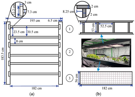
Figure 2. Growth structure dimensions: (a) front view of the schematic and (b) isometric view of rack.

2.2.3. LED Distribution with Light Recipe

The LED distribution was established for an R/B 3:1 ratio light recipe, considering 30% of the PPF efficiency and a minimum threshold of 150 μmol s⁻¹. The number of LEDs was determined based on the model; for a 75% emission in R, 64 LEDs were required for LED 1 and LED 2, while 144 were needed for LED 3. For the 25% emission in B, 25 LEDs were used for LED 4, and 49 were employed for both LED 5 and LED 6. The LEDs were distributed over a 50 × 50 cm area without overlapping, ensuring full coverage of the lighting mounting zone within the growth structure.

2.3. Optical Modeling

2.3.1. LED Modeling as Light Source

The optical profiles of the LEDs were modeled in TracePro^® using spectral emission graphs, emission angles, and Rflux values for each model, obtained from their datasheets. The specific formats of the spectral emissions in R and B, as well as the emission angles of the LEDs, are described in detail in Figure S1 of Section SI of the Supplementary Material of this work.

2.3.2. Crop Area Modeling

Figure 3a shows the arrangement of the modeled components in the growth structure, with three light sources of 50 × 50 cm placed over a cultivation area of 56 × 182 cm. Additionally, reflective walls of 10 × 56 cm and 10 × 165.5 cm were included around the light sources to increase irradiance (Figure 3b), establishing two scenarios for one level of the growth rack: ‘open’ (O), without reflective elements, and ‘closed’ (C), with reflective walls. In this context, the labels (1)–(3) correspond to the mounting areas of lamps 1, 2, and 3; (4) indicates the height between the emitters and the receiver; (5) represents the total cultivation area, and (6) refers to the reflective walls.

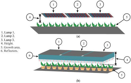
Figure 3. Growth rack level component modeling: (a) scenery O and (b) scenery C.

2.3.3. LED Spatial Distribution Modeling

Based on the distribution established in Section 2.2.3, the modeling of three LED distributions (D1, D2, and D3) was carried out to determine the position that maximizes the irradiated area, where D1 and D2 are common distributions in commercial lamps and D3 is a proposal. Each configuration was adapted to the mounting area, ensuring adequate spacing between the devices to minimize physical and electronic interference in the final lamp design. The LED spatial distributions are detailed in this section.

LED Layout 1 (D1)

In configuration D1, the R and B LEDs were symmetrically distributed within the light source area (50 × 50 cm). In the R LED distribution, 64 LEDs were used for LED 1 and LED 2, while 144 were required for LED 3. The B LED distribution, 25 LEDs were employed for LED 4, while 49 were used for both LED 5 and LED 6, ensuring the R/B 3:1 ratio. The D1 arrangement and the distance between the elements can be observed in the Supplementary Material in Figure S2 of Section SII.

LED Layout 2 (D2)

The location of the LEDs for the D2 configuration and their spacing, maintaining the same number of emitters used in D1 but with an asymmetric distribution, is illustrated in Figure S3 in the Supplementary Material. The LED spacing was preserved under the same conditions as in D1. The same distribution in R was shared by LED 1 and LED 2, while in B, it was identical in LED 5 and LED 6.

LED Layout 3 (D3)

The arrangement of the light emitters in the D3 distribution is shown in the Supplementary Material in Figure S4, where the space between each element is observed. In this design an empty space was strategically created at the center of the light source to reduce light emission in that area and enhance peripheral irradiance, while maintaining the established light recipe proportions as well as the number of elements per spectrum.

2.4. Optical Simulation Environment

Table 2 summarizes the experimental design, detailing the independent variables (factors and levels), controlled parameters, and response variables used to evaluate lighting performance. This structure was developed to assess the effects of LED type, spatial arrangement, and lamp height on radiation uniformity and optical efficiency.

Table 2. Alternative of experimental design.

Category	Element	Description/Levels
Independent variable	LED type	Blue LED, Red LED
	Mounting height	30 cm, 35 cm
	Spatial configuration	Aligned layout, Offset layout, proposal
	Environment scenario	Open area, enclosed box
Controlled conditions	Spectral composition	75% Red:25% Blue
	Power input	Constant (between 418.8 and 449.4 W)
	Simulation grid resolution	Fixed (1.42 cm × 1.42 cm cells)
Dependent variable	PPFD	μmol·m−2·s−1
	Uniformity index (u)	Dimensionless (0–1)
	Optical efficiency (ηₒ)	% of emitted flux captured over the target area

2.4.1. Optical Simulation Parameters

The experimental design considered the six LED with spectral emissions in R and B, as well as the modeled distributions (D1, D2 and D3). Each distribution included three light sources (lamps) to irradiate the cultivation area. Reflectance conditions in the area (scenarios O and C) and the height between the emitters and the receiving area were also included.

Heights

Based on the dimensions of the growth structure (Figure 3a), the mounting heights of 30 and 35 cm were selected based on operational ranges commonly reported in controlled-environment agriculture. Several studies highlight that distances between 25 and 40 cm optimize light uniformity, energy use, and canopy coverage in LED systems [5,29,30]. This range allows sufficient PPFD delivery while minimizing energy losses due to beam divergence.

Irradiance Conditions

The irradiance conditions were configured in TracePro^®, with each LED programmed to emit 100,000 rays, a quantity selected after a thorough convergence analysis, which resulted in a variation of approximately 0.1% between simulations. The total cultivation area was set with 100% absorbance, while the sidewalls and the lamp body had reflectance values of 90% and 50%, respectively, within the 400 to 700 nm range. Figure 4 shows the experimental design used to evaluate irradiance at one level of the growth rack with the 75R + 25B light recipe.

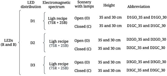
Figure 4. Design of experiments at the growth rack level.

2.4.2. Optical Simulation Execution

The simulations, following the diagram in Figure 4, were initiated with the combination of LED 1 + LED 4 (CLED_1) due to its lower number of LEDs, followed by LED 2 + LED 5 (CLED_2), and finally by LED 3 + LED 6 (CLED_3), this last combination requires the highest computational demand (the LED combinations were made due to the number of LEDs used). For each simulation, irradiance maps were produced, which include key metrics and represent, using a color scale, the distribution, intensity, and uniformity of irradiance in the same area (see Figure S5 in Supplementary Material). Additionally, .txt files were generated containing radiant flux matrices of 128 × 128 pixels (16,384 values), representing the light distribution in the cultivation area. Among the collected metrics are the dimensions of the target area, total number of incident rays, ηₒ, total radiant flux (Tflux), and average radiant flux per square meter (Ave).

2.4.3. Comparison Criteria

The study employs key radiometric and photometric concepts to evaluate light distribution and efficiency. Radiant flux (W) refers to the total energy emitted per unit of time, whereas photon flux (μmol s⁻¹) quantifies the number of photons within PAR range (400–700 nm), irrespective of their individual energy [1]. The PPFD measures how many of these photons imping a square meter per second and serves as the standard metric for quantifying incident light in horticultural systems [2]. Since photon energy is inversely proportional to wavelength, as described by the equation E = hc/λ, blue photons (~450 nm) carry a substantially higher amount of energy than red photons (~660 nm), even though both are counted equally in photon flux measurements [5]. As a result, two light sources the same PPFD can demonstrate notable differences in power consumption. This highlights the importance of distinguishing between energy efficiency (J J⁻¹) and photon efficiency (μmol J⁻¹) when analyzing LED lighting systems [4]. In this context, the study defines the ηₒ as the fraction of the total emitted radiant flux that is effectively impinging over the cultivation area, excluding losses due to reflection, scattering, or geometric inefficiencies [31]. For further definitions, see Table S1 in the Supplementary Material.

To ensure a fair comparison between the distributions and LEDs analyzed in this study, various parameters were considered for the evaluation of the light sources. The analysis began with the examination of the number of emitters, luminous intensity, electrical energy consumption, and total purchase cost of LEDs. Subsequently, the evaluation was based on the parameters ηₒ, Tflux, and Ave, obtained from the irradiance maps for D1, D2, and D3 (Figure S5), along with the values of u and average uniformity (uav), calculated from the energy of a photon (E) at a specific wavelength (λ = λ_peak), as defined in Equation (1), where h is Planck’s constant (6.626 × 10⁻³⁴ J∙s) and c is the speed of light (299,792,458 m·s⁻¹),

$$E= {\displaystyle \frac{hc}{\lambda }} .$$

(1)

Once E was calculated, it was linked to Avogadro’s number (Nₐ = 6.02214087 × 10²³ mol⁻¹) to obtain Ef, according to Equation (2),

$$E_f=E\times N_a.$$

(2)

The calculated value of Ef and the Tflux obtained from the irradiance map were used to calculate the PPF emitted per wavelength using Equation (3), ensuring a minimum emission of 150 μmol s⁻¹ with a ratio of 75% R + 25% B in the light recipe,

$$PPF={\displaystyle \frac{TFlux}{E_f}}.$$

(3)

The relationship between Ave and Ef was used to calculate PPFD, a measure of PAR, using Equation (4)

$$PPFD={\displaystyle \frac{Ave}{E_f}}.$$

(4)

The correlation between the flux values (PPFD_data) of each pixel in the target area and the maximum flux (PPFD_max) was used to calculate uniformity (u) and generate the graph according to Equation (5)

$$u={\displaystyle \frac{{PPFD}_{data}}{{PPFD}_{max}}} .$$

(5)

Finally, uav was obtained by summing each calculated u value and applying Equation (6), where u_i is each calculated uniformity value, and n is the total number of values.

$$uav={\displaystyle \frac{1}{n}} \sum _{i=1}^n{u}_i.$$

(6)

2.4.4. Statistical Analysis

The data were analyzed using a one-way analysis of variance (ANOVA) to detect significant differences among LED distributions. Post hoc mean comparison tests, such as Tukey and Fisher, were applied with a significance level of p < 0.05 [32]. The analyses were conducted using the statistical software MINITAB 17, and the results were expressed as the mean ± standard deviation (SD) of three independent LED distributions, following statistically validated methodologies for experimental studies [33]. In addition, the Shapiro–Wilk homogeneity test and the Levene variance test were performed [34].

3. Results

The design of a uniform radiation system for indoor crops is crucial to preventing differences in development during the vegetative stage, as well as in nutritional content. In this proposal, different LED irradiation configurations were evaluated through simulations conducted with TracePro^®, considering various LED with emissions in R and B, spatial distributions, and the same reflectance conditions. The obtained results are presented below, analyzing the configuration in terms of the number of LEDs, electrical energy consumption, and total purchase cost of LEDs. The modeled LED distributions (D1, D2 and D3) were compared based on the amount of emitted radiation and the uniformity of irradiance distribution in the cultivation area, allowing the identification of optimal conditions.

3.1. Comparison by Total Values of Emission and Electrical Energy Consumption

Figure 5a–d compares three LED configurations (CLED_1, CLED_2, CLED_3), all with a R/B 3:1 ratio and the number of LEDs required for equivalent radiance across them. Figure 5a illustrates an increase in the number of LEDs from 267 in CLED_1 to 579 in CLED_3, accompanied by a rise in total system cost (from USD 239.8 to 969.4). Figure 5b shows a corresponding increase in power consumption, from 418.8 to 449.4 W. In Figure 5c, PPF values remain relatively constant (1550–1582 µmol s⁻¹), indicating minimal gains in photon output despite the higher diode density. Figure 5d highlights the relationship between PPF and energy consumption, demonstrating that increased light output requires disproportionately higher energy and financial investment. Together, these findings underscore the trade-off between diode quantity, system efficiency, and cost-effectiveness—showing that while increased emitter density yields slight improvements in photon flux, it significantly elevates both operational and capital demands. Further details on spectral composition and configuration parameters are available in Table S2.

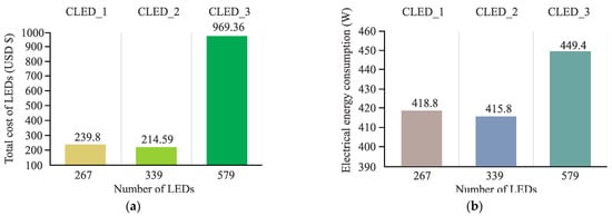
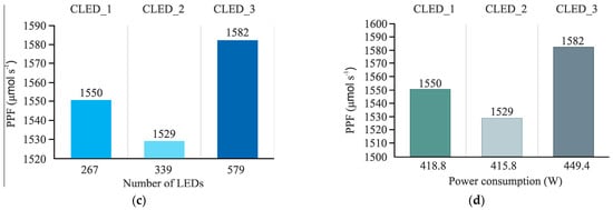
Figure 5. Graphical comparisons of characteristics on LED lamp group with R+B electromagnetic spectrum emission: (a) Number of LEDs vs. total cost of LEDs, (b) Number of LEDs vs. electrical energy consumption, (c) Number of LEDs vs. PPF and (d) power consumption vs. PPF.

For the comparison between the O and C distribution scenarios at heights of 30 and 35 cm, the λ_peak value from Table 1 was required to calculate E for each electromagnetic spectrum using Equation (1), and subsequently E_f with Equation (2). Based on the generated irradiance maps, Tflux and Ave were determined to calculate the PPF with Equation (3) and the average PPFD using Equation (4) with E_f. In this way, the average PPFD per spectrum and its percentage in the recipe total average PPFD were obtained. The PPFD values for scenario O are presented in Table 3, while those for scenario C are shown in Table 4, along with the total LED count for each LED combination. However, this improvement did not translate into proportional energy efficiency gains, since total power consumption and LED counts remained constant across both setups. CLED_1 achieved the highest PPFD in both conditions (915 and 1057 µmol m⁻² s⁻¹ for O and C, respectively), whereas CLED_3, despite its greater diode density and energy demand (449.4 W), yielded the lowest PPFD (769 and 870 µmol m⁻² s⁻¹). These results confirm that optimizing the optical design and distribution geometry of the luminaire is more effective for enhancing photon-use efficiency than merely increasing emitter quantity or power input. The comparison graph of the combinations, distributions, and scenarios, considering the data in Table 3 and Table 4 is detailed in Figure S6 of Section SIV of the Supplementary Material.

Table 3. PPFD behavior of the R+B spectral emission lamp group with different LED spatial distribution, applied on 56 × 182 cm area at mounting heights of 30 and 35 cm, scenario O.

LED Combinations	Total LED	LED Distribution	Height	R		B		Recipe
				Average PPFD (μmol m−2s−1)	% Recipe	Average PPFD (μmol m−2s−1)	% Recipe	Total Average PPFD (μmol m−2s−1)
CLED_1	267	D1	30	670	73.11	246	26.89	915
	267	D2	30	669	73.19	245	26.81	914
	267	D3	30	656	73.54	236	26.46	892
CLED_2	339	D1	30	653	75.14	216	24.86	869
	339	D2	30	652	75.12	216	24.88	868
	339	D3	30	639	75.09	212	24.91	851
CLED_3	579	D1	30	654	75.61	211	24.39	865
	579	D2	30	653	75.58	211	24.42	864
	579	D3	30	645	75.62	208	24.38	853
CLED_1	267	D1	35	606	73.19	222	26.81	828
	267	D2	35	606	73.28	221	26.72	827
	267	D3	35	595	73.55	214	26.45	809
CLED_2	339	D1	35	592	75.22	194	24.65	787
	339	D2	35	592	75.32	194	24.68	786
	339	D3	35	580	75.13	191	24.74	772
CLED_3	579	D1	35	589	75.51	190	24.36	780
	579	D2	35	589	75.61	190	24.39	779
	579	D3	35	582	75.68	187	24.32	769

Table 4. PPFD behavior of the R+B spectral emission lamp group with different LED spatial distribution, applied on 56 × 182 cm area at mounting heights of 30 and 35 cm, scenario C.

LED Combinations	Total LED	LED Distribution	Height	R		B		Recipe
				Average PPFD (μmol m−2s−1)	% Recipe	Average PPFD (μmol m−2s−1)	% Recipe	Total Average PPFD (μmol m−2s−1)
CLED_1	267	D1	30	769	72.75	288	27.25	1057
	267	D2	30	768	72.66	289	27.34	1057
	267	D3	30	767	72.84	286	27.16	1053
CLED_2	339	D1	30	760	74.07	267	26.02	1026
	339	D2	30	760	74.07	266	25.93	1026
	339	D3	30	758	74.02	267	26.07	1024
CLED_3	579	D1	30	712	73.15	261	26.85	972
	579	D2	30	712	73.25	260	26.75	972
	579	D3	30	705	73.06	260	26.94	965
CLED_1	267	D1	35	695	72.77	260	27.23	955
	267	D2	35	695	72.70	261	27.30	956
	267	D3	35	695	72.85	259	27.15	954
CLED_2	339	D1	35	688	74.11	240	25.89	927
	339	D2	35	689	74.14	240	25.86	928
	339	D3	35	687	74.11	240	25.89	927
CLED_3	579	D1	35	641	73.26	234	26.74	875
	579	D2	35	641	73.26	234	26.74	875
	579	D3	35	636	73.10	234	26.90	870

3.2. Comparison by Data Array Values

Using the information obtained from the .txt files generated in the TracePro^® simulations and Equation (4), irradiance graphs were created for the different LED distributions at heights of 30 and 35 cm above the longest side of the cultivation area. Regarding D1 and D2, similar behaviors are observed with the same LED combination, where PPFD increases as the height decreases, while D3 maintains the lowest PAR value, regardless of the scenario and height used. The behavior of the PPFD can be observed in depth in Figure S7 of Section SV of the Supplementary Material.

The u value for each distribution was calculated using Equation (5), based on the maximum of the matrix and the irradiance data. Figure 6 shows that the behavior of the u values is similar; however, while scenario O provides a u value between 70% and 80% at a distance of 19 to 28 cm (see blue lines of Figure 6a,c), scenario C presents slight increases of around 1% in the results as it offers between 70% and 80% of u at a distance of 17 to 22 cm at both heights (see blue lines of Figure 6b,d). The D1 and D2 distributions are observed to be similar across LED combinations and scenarios, while D3 remains different, showing a slight improvement in u regardless of height, scenario, or LED.

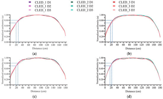
Figure 6. Comparison of irradiance uniformity in scenarios O and C at two heights: (a) scenery O at 35 cm, (b) scenery C at 35 cm, (c) scenery O at 30 cm and (d) scenery C at 30 cm.

The distributions were also compared through Tflux, Ave, and η_o, which were retrieved from the irradiance maps, calculating the total average PPFD and uav using Equation (6). The data collection is shown in Table S3 in the Supplementary Material, where is observed that the three spatial distributions exhibit similar u value, ranging between 68% and 71%, with minimal differences in total average PPFD within the same LED combination, ensuring PPFD values that contribute to the production of crops with better growth characteristics. Additionally, when the emitter-receiver distance is reduced, the PPFD values increase, and the differences between distributions decrease in scenario C, maintaining u. Figure 7 graphically shows that total average PPFD is higher in scenario C for all LED combinations, with minimal differences between the LED distributions. The highest values are presented by CLED_1 in both scenarios (915 in scenario O and 1057 μmol m⁻² s⁻¹ in scenario C), while CLED_2 and CLED_3 are similar in scenario O (between 865 and 869 μmol m⁻² s⁻¹). However, in scenario C, the lowest values are exhibited by CLED_3, even with reflective walls (972 μmol m⁻² s⁻¹).

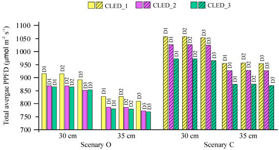
Figure 7. Comparison of total average PPFD among different spatial LED arrangements across both scenarios and at two mounting heights.

3.3. Comparison by Irradiance Maps

The three LED combinations were evaluated using the irradiance maps generated in the simulations, considering spatial distribution, height, and scenario. According to the above, a minimum PPFD value between 200 and 300 μmol m⁻² s⁻¹ is maintained at the edges of the cultivation area, depending on the LED combination used, which contributes to the production of fresh and dry biomass [9]. Similarly, an increase of approximately 200 μmol m⁻² s⁻¹ in the maximum PPFD value is observed under the closed scenario. Distributions D1 and D2 are characterized by similar behavior, while distribution D3 is distinguished by the most homogeneous uniformity compared to the others, regardless of the mounting height. The evaluation of the PPFD behavior of the LED distributions in the different irradiance maps can be observed in depth in Section SVI of the Supplementary Material.

3.4. Comparison by Statistical Data Analysis

The analysis of variance (ANOVA) for the performance of the different LED spatial distributions (D1, D2, and D3) was conducted based on the metrics obtained from the irradiance simulations. The main response variables considered were the LED combinations, distribution, scenarios, height, and average PPFD. Table 5 presents the variables and the results after applying Tukey’s multiple comparison test [32], which was used to identify which configurations exhibited significant differences. Significant differences were found in all factors except for LED distribution. These data can also be verified through the column of Fisher values [33], where the highest value is presented by the scenarios, followed by height, LED combinations, and finally, LED spatial distribution. Normality and homogeneity of variance tests indicated that for the probability of response to irradiance (p > 0.100), the response to brand and R+B LED combination (p > 0.987), the response to distance and R+B LED combination (p > 0.979), and the response to distance and scenarios (p > 0.473), all p-values exceeded 0.05. This suggests that the data satisfy the assumptions of normality and homogeneity of variance. Detailed performance plots of the variance tests are provided in Figure S12, Section SV of the Supplementary Material.

Table 5. Variance Analysis of the performance of the different LED distributions.

Factors	Degrees of Freedom	Adjusted Treatments	Tight Measurements	Fisher Values	p Values (Tukey)
Model	6	259,454	43,242	244.56	0.000
Linear relationship	6	259,454	43,242	244.56	0.000
LED combinations	2	25,296	12,648	71.53	0.000
Scenarios	1	158,802	158,802	898.11	0.000
Height	1	74,620	74,620	422.01	0.000
LED spatial distribution	2	735	368	2.08	0.143
Error	29	5128	177
Total	35	264,582

In the Pareto diagram of Figure 8, the level of difference is shown, confirming that the most significant impact is due to the scenarios, followed by height, while the LED combinations has a lesser influence. This is because, initially, the LED distributions were designed to emit a comparable amount of PPF, confirming that the number of LEDs is adjusted to ensure an almost identical luminous flux emission. Regarding the LED distributions, this is the factor with the least dispersion according to the average PPFD values used in the statistical test. A final comparison based on the irradiated area and irradiance level still needs to be analyzed, which is described in Section 3.5.

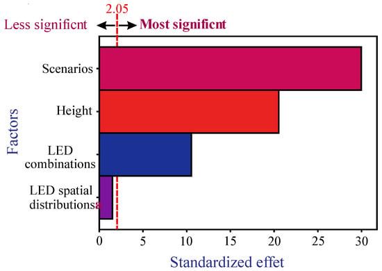
Figure 8. Pareto diagram of standardized effects (α = 0.05).

3.5. Comparison by Irradiance Area

The irradiance area comparison was conducted through the analysis of PPFD data classified by ranges, using the irradiance map matrices. For this analysis, a height of 30 cm was exclusively considered, as it records the highest values. Each data point represents a pixel with an area equivalent to 2.0164 × 10⁻⁴ m² within the total growth rack level (1.0192 m²). The PPFD value range and the percentage of the irradiated area for the three LED combinations, considering the different distributions and scenario O, is presented in Table S4 of the Supplementary Material. It is observed that distributions D1 and D2 provide a similar PPFD distribution within the same area, while in distribution D3, the maximum PPFD value decreases, increasing the total irradiated area within the 800 to 1200 μmol m⁻² s⁻¹ range. This suggests that D3 provides lower intensity but higher u in irradiance. Additionally, a significant percentage of PPFD in the 1201 to 1600 μmol m⁻² s⁻¹ range is observed for CLED_1.

Details of the irradiated area in scenario C are also shown in the Supplementary Material in Table S5. It is observed that between 75% and 78% of the total PPFD in the irradiated area for CLED_1 and CLED_2 falls within the range of 800 to 1600 μmol m⁻² s⁻¹ across the three distributions, while for CLED_3, this range remains between 800 and 1300 μmol m⁻² s⁻¹. Distributions D1 and D2 show a similar irradiated area across the three LED combinations, while distribution D3 reduces its percentage at the highest PPFD values but slightly increases it within lower irradiance ranges. This suggests that D3 offers a slight increase in u. Additionally, a more stable u is maintained by CLED_3 compared to the other LED combinations, regardless of the spatial distribution used.

4. Discussion

The results of this study indicate that the use of walls with 90% reflectance, without employing fluorescent coatings, as in Yalçın and Ertürk [15], systems with Fresnel lenses used by Vu et al. [16], or incorporating a triangular prism into the LED array base plate as implemented by K. Xu et al. [20] significantly improves the utilization of average PPFD from LED light sources compared to not using them. This translates into an increase of up to 18% in distributions D1 and D2, and up to 20% in D3, depending on the LED combination used. Additionally, it is observed that the irradiation uniformity remains slightly at 70% at both heights, which contributes to the production of fresh and dry biomass, as well as greater leaf development in lettuce and basil crops, according to Pennisi et al. [9], or to homogeneous growth in cucumber and watermelon seedlings, as indicated Lee et al. [17]. Without reflective walls, differences between LED distributions of the same combination are more evident. With reflective walls, the difference in total average PPFD is reduced to less than 10 μmol m⁻² s⁻¹, making the choice of a specific distribution less relevant.

The lamp size must be adjusted to the application area to maximize the distribution of irradiance without having a closed incubator-type space as in J. Bai et al. [19]. The amount of PPFD is increased by up to 10% when reducing the distance from 35 to 30 cm, regardless of the scenario, LED combination or spatial distribution used, enhancing the homogeneity of irradiance in the cultivation area, contrary to what was stated by Rakutko and Rakutko [22].

Unlike the findings of Boros et al. [35], which reported non-homogeneous irradiance maps due to the use of different LED light sources, the results suggest that an LED distribution with empty spaces in the central area of the light source positioning zone (D3) reduces the PPFD difference between the center and the perimeter of the cultivation area by 4% to 8% in scenario O and by 2.7% to 6.5% in scenario C, improving irradiance homogeneity. This minimizes production differences associated with a suboptimal arrangement of luminaires in vertical farms. The D3 distribution differs significantly from D1 and D2, which exhibit similar behavior at any height. Although D3 reduces total PPFD, it maintains better uniformity in the irradiated area at a height and area greater than that reported by J. Mei and J. Zou [18].

The simulations provide strong evidence of the irradiance distribution for a light recipe of 75% R + 25% B across different spatial arrangements of horticultural LEDs, serving as a valuable reference for optimizing indoor plant growth systems. However, while these results contribute to analyzing the uniformity of LED lighting parameters—an understudied aspect in vertical farming—the irradiance map values are derived from simulations of commercial LEDs specialized in horticulture under ideal conditions. The study assumes a specific growth shelf size, as well as optimal radiance and electrical energy consumption values. Consequently, the energy impact or potential losses due to real-world experimental setups have not been evaluated.

Although this study centers on optical simulation, numerous experimental investigations have demonstrated that light uniformity plays a crucial role in plant growth, photosynthesis, and biomass distribution. For instance, Sheibani et al. [29] and Lanoue et al. [5] reported that non-uniform light distribution can cause uneven canopy development, while Pennisi et al. [9] observed that uniform and consistent illumination enhances yield and reduces waste. Similarly, Ali [36] showed that controlled modulation of red and blue light can influence plant morphology and metabolite production. Collectively, these findings underscore the importance of optimizing spatial light distribution in the optical design stage.

Future research could address these limitations by assessing energy efficiency and losses in practical applications. Additionally, investigating the spatial distribution of horticultural LEDs with ultraviolet A (UV-A), green (G), and near-infrared (NIR) wavelengths for growth racks, which are also very important in the development of the plant, could provide new insights into optimizing radiation to enhance crop yield and quality.

5. Conclusions

The design and development of LED lamps for indoor crop environments require careful planning to achieve appropriate lighting according to the specific needs of plants. Defining a light recipe requires consideration of PPF, wavelength and the emission angle of each horticultural LED. This task becomes more complex when different LEDs are used, as small variations in wavelength can alter PPF and modify the number of LEDs needed. Electrical connectivity, energy consumption, and lamp manufacturing costs are directly affected by these factors. The size and distribution of the lamp must be adapted to the cultivation area to ensure a uniform distribution of irradiance. In environments without reflective surfaces, differences between LED configurations with similar characteristics are noticeable. However, when reflective walls are used, the difference in irradiance is reduced, making the choice of a specific distribution less relevant. An effective strategy for improving light uniformity is to reduce the number of LEDs in the central zone of the lamp, thereby decreasing the PPFD concentration in the center and achieving a more homogeneous distribution over the cultivation area. Some key points to highlight from this work are:

-

Under the same light recipe, maximum differences per lamp can be observed in the following parameters: electrical energy consumption (8.08%), photosynthetic photon flux (3.47%), purchase cost of LEDs (351.72%), and number of components (116.85%).

-

The use of reflective walls increased the average photosynthetic photon flux density by up to 18% in LED spatial distributions 1 and 2, and close to 20% in distribution 3, compared to a scenario without reflective walls.

-

LED spatial distribution 3 can reduce the difference in photosynthetic photon flux density between the center and the perimeters of the target area by 4% to 8% in scenario O, and by 2.7% to 6.5% in scenario C (to increase irradiance homogeneity).

-

Reducing the height from 35 cm to 30 cm increased the photosynthetic photon flux density by up to 10%.

In summary, the development of LED lamps for indoor crops should focus on improving energy efficiency, ensuring a uniform distribution of irradiance, and adapting to different cultivation dimensions. The simulation of various spatial LED configurations is considered a valuable tool for designing lighting systems that meet the needs of producers. This approach facilitates plant growth control and serves as a reference for the construction of customized lamps in different indoor cultivation environments.

References

- Villagran, E.; Espitia, J.J.; Rodriguez, J.; Gomez, L.; Amado, G.; Baeza, E.; Aguilar-Rodríguez, C.E.; Flores-Velazquez, J.; Akrami, M.; Gil, R.; et al. Use of Lighting Technology in Controlled and Semi-Controlled Agriculture in Greenhouses and Protected Agriculture Systems—Part 1: Scientific and Bibliometric Analysis. Sustainability 2025, 17, 1712. [Google Scholar] [CrossRef]
- Pannico, A.; Arouna, N.; Fusco, G.M.; Santoro, P.; Caporale, A.G.; Nicastro, R.; Pagliaro, L.; De Pascale, S.; Paradiso, R. Enhancing tuber yield and nutraceutical quality of potato by supplementing sunlight with LED red-blue light. Front. Plant Sci. 2025, 16, 1517074. [Google Scholar] [CrossRef] [PubMed]
- Inthima, P.; Supaibulwatana, K. Green LEDs lighting enhances vigorous growth and boosts bacoside production in hydroponically cultivated Bacopa monnieri (L.) Wettst. Hortic. Environ. Biotechnol. 2025, 66, 491–507. [Google Scholar] [CrossRef]
- Khan, Q.; Wang, A.; Li, P.; Hu, J. Quantum Dots Illuminating the Future of Greenhouse Agriculture. Adv. Sustain. Syst. 2025, 9, 2401015. [Google Scholar] [CrossRef]
- Lanoue, J.; Hao, X.; Vaštakaitė-Kairienė, V.; Marcelis, L.F.M. Physiological growth responses to light in controlled environment agriculture. Front. Plant Sci. 2024, 15, 1529062. [Google Scholar] [CrossRef]
- Asgari, N.; Basdeo, A.; Givans, J.; Pearce, J.M. Lighting and Revenue Analysis of Grow Lights in Agrivoltaic Agrotunnel for Lettuces and Swiss Chard. SSRN. 2025. Available online: https://papers.ssrn.com/sol3/papers.cfm?abstract_id=5104787 (accessed on 1 October 2025).
- Despommier, D. Vertical farming: A holistic approach towards food security. Front. Sci. 2024, 2, 1473141. [Google Scholar] [CrossRef]
- Paucek, I.; Appolloni, E.; Pennisi, G.; Quaini, S.; Gianquinto, G.; Orsini, F. LED Lighting Systems for Horticulture: Business Growth and Global Distribution. Sustainability 2020, 12, 7516. [Google Scholar] [CrossRef]
- Pennisi, G.; Pistillo, A.; Orsini, F.; Cellini, A.; Spinelli, F.; Nicola, S.; Fernandez, J.A.; Crepaldi, A.; Gianquinto, G.; Marcelis, L.F.M. Optimal light intensity for sustainable water and energy use in indoor cultivation of lettuce and basil under red and blue LEDs. Sci. Hortic. 2020, 272, 109508. [Google Scholar] [CrossRef]
- Wang, Y.; Li, T.; Chen, T.; Zhang, X.; Taha, M.F.; Yang, N.; Mao, H.; Shi, Q. Cucumber Downy Mildew Disease Prediction Using a CNN-LSTM Approach. Agriculture 2024, 14, 1155. [Google Scholar] [CrossRef]
- Rouphael, Y.; Ciriello, M. Vertical farming: A toolbox for securing vegetable yield for the food of the future. Front. Sci. 2024, 2, 1491748. [Google Scholar] [CrossRef]
- Asiabanpour, B.; Estrada, A.; Ramirez, R.; Downey, M.S. Optimizing Natural Light Distribution for Indoor Plant Growth Using PMMA Optical Fiber: Simulation and Empirical Study. J. Renew. Energy 2018, 2018, 9429867. [Google Scholar] [CrossRef]
- Bo, Y.; Zhang, Y.; Zheng, K.; Zhang, J.; Wang, X.; Sun, J.; Wang, J.; Shu, S.; Wang, Y.; Guo, S. Light environment simulation for a three-span plastic greenhouse based on greenhouse light environment simulation software. Energy 2023, 271, 126966. [Google Scholar] [CrossRef]
- Park, Y.; Runkle, E.S. Far-red radiation promotes growth of seedlings by increasing leaf expansion and whole-plant net assimilation. Environ. Exp. Bot. 2017, 136, 41–49. [Google Scholar] [CrossRef]
- Yalçın, R.A.; Ertürk, H. Improving crop production in solar illuminated vertical farms using fluorescence coatings. Biosyst. Eng. 2020, 193, 25–36. [Google Scholar] [CrossRef]
- Vu, D.T.; Nghiem, V.T.; Tien, T.Q.; Hieu, N.M.; Minh, K.N.; Vu, H.; Shin, S.; Vu, N.H. Optimizing optical fiber daylighting system for indoor agriculture applications. Sol. Energy 2022, 247, 1–12. [Google Scholar] [CrossRef]
- Lee, H.J.; Moon, Y.H.; An, S.; Sim, H.S.; Woo, U.J.; Hwang, H.; Kim, S.K. Determination of LEDs arrangement in a plant factory using a 3D ray-tracing simulation and evaluation on growth of Cucurbitaceae seedlings. Hortic. Environ. Biotechnol. 2023, 64, 765–774. [Google Scholar] [CrossRef]
- Mei, J.; Zou, J. Optimizing LED Array Irradiance Uniformity with a Particle Swarm Optimization-Based Scheme: Application in a Parallel Photoreactor. Appl. Opt. 2024, 63, 4336–4344. [Google Scholar] [CrossRef] [PubMed]
- Bai, J.; Li, X.; Hu, L.; Wei, Y.; Gao, T.; Xu, X.; Sun, X. Research on illumination uniformity in edible mushrooms incubator with genetic algorithm. Optik 2021, 239, 166862. [Google Scholar] [CrossRef]
- Xu, K.; Zeng, L.; Li, Z.; Chen, H.; Qiao, Z.; Qu, Y.; Liu, G.; Li, L. Research on illumination uniformity of LD andLED hybrid lighting system applied to plant growth. Appl. Opt. 2022, 61, 10717–10726. [Google Scholar] [CrossRef]
- LAMBDA, R.C. TracePro Software for Design and Analysis of Illumination and Optical Systems. Available online: https://lambdares.com/tracepro (accessed on 20 March 2025).
- Rakutko, S.A.; Rakutko, E.N. Assessment of Lighting Uniformity as a Factor of Energy Efficiency in Greenhouse Horticulture. Eng. Technol. Syst. 2021, 31, 470–486. [Google Scholar] [CrossRef]
- Gao, Q.; Liao, Q.; Li, Q.; Yang, Q.; Wang, F.; Li, J. Effects of LED Red and Blue Light Component on Growth and Photosynthetic Characteristics of Coriander in Plant Factory. Horticulturae 2022, 8, 1165. [Google Scholar] [CrossRef]
- OSRAM. GH CSSRM5.24. Available online: https://look.ams-osram.com/m/b1e8ccf53e9cd4/original/GH-CSSRM5-24.pdf (accessed on 3 June 2025).
- SAMSUNG. LH351H 2W 660nm Deep Red Ver.2. Available online: https://download.led.samsung.com/led/file/resource/2022/05/Data_Sheet_LH351H_660nm_Red_V2_Rev.3.7.pdf (accessed on 19 March 2025).
- CREE. XLamp® XP-G3 LEDs. Available online: https://downloads.cree-led.com/files/ds/x/XLamp-XPG3.pdf (accessed on 21 March 2025).
- OSRAM. GD CSSRM3.14. Available online: https://look.ams-osram.com/m/56f334aabb38c31/original/GD-CSSRM3-14.pdf (accessed on 20 March 2025).
- SAMSUNG. LH351H 450 nm Blue. Available online: https://download.led.samsung.com/led/file/resource/2023/01/Data_Sheet_LH351H_450nm_Blue_Rev.3.8.pdf (accessed on 19 March 2025).
- Sheibani, F.; Bourget, M.; Morrow, R.C.; Mitchell, C.A. Close-canopy lighting, an effective energy-saving strategy for overhead sole-source LED lighting in indoor farming. Front. Plant Sci. 2023, 14, 1215919. [Google Scholar] [CrossRef]
- Wong, T.I.; Zhou, X. Uniform Lighting of High-Power LEDs at a Short Distance to Plants for Energy-Saving and High-Density Indoor Farming. Photonics 2024, 11, 394. [Google Scholar] [CrossRef]
- Chen, X.; Hou, T.; Liu, S.; Guo, Y.; Hu, J.; Xu, G.; Ma, G.; Liu, W. Design of a Micro-Plant Factory Using a Validated CFD Model. Agriculture 2024, 14, 2227. [Google Scholar] [CrossRef]
- Yamada, J.T.; Viana, R.S.E.; Santos, R.R.; de Carvalho, C.P.; de Almeida, M.G.D.; de Barros, J.G.M.; Sampaio, N.A.S. Use of factorial design with significant interaction and Tukey’s Test in agricultural and environmental experiments. Rev. Gestão Secr. (Manag. Adm. Prof. Rev.) 2023, 14, 9815–9828. [Google Scholar] [CrossRef]
- Arif, M.; Ameen, K.; Rafiq, M. Factors affecting student use of Web-based services. Electron. Libr. 2018, 36, 518–534. [Google Scholar] [CrossRef]
- Boynton, G.M. Introduction to Statistics and Data Analysis. Available online: https://courses.washington.edu/psy524a/_book/tests-for-homogeneity-of-variance-and-normality.html (accessed on 4 June 2025).
- Boros, I.F.; Székely, G.; Balázs, L.; Csambalik, L.; Sipos, L. Effects of LED lighting environments on lettuce (Lactuca sativa L.) in PFAL systems—A review. Sci. Hortic. 2023, 321, 112351. [Google Scholar] [CrossRef]
- Ali, A. Basic and Applied Research Approaches for Optimizing the Use of Artificial Light in Vegetable Crops. Ph.D. Thesis, Università degli Studi di Milano, Milano, Italy, 2024. [Google Scholar]
Disclaimer/Publisher’s Note: The statements, opinions and data contained in all publications are solely those of the individual author(s) and contributor(s) and not of MDPI and/or the editor(s). MDPI and/or the editor(s) disclaim responsibility for any injury to people or property resulting from any ideas, methods, instructions or products referred to in the content. |
© 2025 by the authors. Licensee MDPI, Basel, Switzerland. This article is an open access article distributed under the terms and conditions of the Creative Commons Attribution (CC BY) license (https://creativecommons.org/licenses/by/4.0/).