Short-Term Power Load Forecasting Under Multiple Weather Scenarios Based on Dual-Channel Feature Extraction (DCFE)

Abstract

Grid security and system dispatch can be compromised by pronounced volatility in power load under extreme meteorological conditions. However, the dynamic and nonlinear interactions between power load and meteorological variables across diverse weather scenarios are not well captured by existing methods, resulting in limited accuracy and robustness. To address this gap, a short-term power load forecasting model with a dual-channel architecture is proposed. Features are extracted in parallel via dual-channel feature extraction (DCFE): the first channel employs an improved Cascaded Multiscale 2D Convolutional Network (CMCNN) to model local fluctuations and global periodicity in the load time series. The second channel derives scenario-aware variable weights using the Maximal Information Coefficient (MIC); meteorological variables are then gated and weighted before being processed by a multi-layer self-attention network to learn global dependencies. Subsequently, dynamic feature-level fusion is achieved through cross-attention, strengthening key interactions between power load and meteorological factors. The fused representation is fed into an Attention-Enhanced Bidirectional Gated Recurrent Unit (AE-BiGRU) to precisely model temporal dependencies across multiple weather scenarios. Experiments on five years of power load and meteorological data from a region in Australia indicate that the proposed method outperforms the best baseline across multiple weather conditions: RMSE, MAE, MAPE, and sMAPE decrease on average by 32.44%, 31.42%, 30.73%, and 31.05%, respectively, while R² increases by 0.034 on average, demonstrating strong adaptability and robustness.

1. Introduction

In recent years, power load forecasting techniques have matured substantially under normal weather conditions. However, the frequency and intensity of extreme weather events have continued to rise due to increasing anomalies in the global climate system. During prolonged heatwaves or cold spells, power load often exhibits pronounced volatility and more complex fluctuation patterns than usual [1]. Such abnormalities exacerbate the risk of supply demand imbalance and pose severe challenges to grid security, stable operation, and supply reliability. Consequently, meeting the requirement for high accuracy short-term forecasting under both normal and extreme weather conditions has become a major research focus in modern power systems [2,3].

Existing approaches to power load forecasting are commonly categorized into statistical, machine learning, and deep learning methods. Statistical techniques include regression analysis [4], autoregressive integrated moving average (ARIMA) [5], and its seasonal extension, SARIMA [6]. These methods offer strong interpretability and computational efficiency under normal weather conditions; however, their performance degrades when confronted with complex nonlinear relationships or load fluctuations induced by extreme meteorological conditions. In particular, classical linear models often struggle to capture abrupt changes, nonlinear characteristics, and multi-factor couplings in load data, and they inadequately characterize the complex interactions between load and exogenous meteorological variables under extreme conditions.

Compared with statistical approaches, machine learning methods provide stronger nonlinear modeling capacity and can discover complex patterns in higher-dimensional feature spaces. Representative methods include support vector regression (SVR) [7,8], random forests (RF) [9], and extreme gradient boosting (XG-Boost) [10]. Although these algorithms mitigate some limitations of traditional statistical models through adaptive learning, they typically rely on fixed feature representations and heuristic assumptions for time-series data, making it difficult to automatically extract latent temporal patterns and complex long-range dependencies.

As power systems grow more complex and forecasting demands increase, deep learning has become a focal area owing to its automatic feature extraction and capacity to model multi-dimensional dynamics. Convolutional Neural Networks (CNNs) extract local spatiotemporal features via receptive fields and have been widely applied to power load forecasting [11]. Gated recurrent units (GRUs), a key RNN variant, propagate historical information through gating and enhance modeling of temporal dynamics [12,13]. Despite their success, CNNs are constrained by fixed receptive fields and thus struggle to capture global dependencies. Although GRUs mitigate gradient vanishing in recurrent networks [14], limitations persist for long sequences. To more fully exploit temporal structure, Bidirectional Gated Recurrent Units (BiGRUs) have been widely adopted in power load forecasting; by integrating forward and backward contexts, BiGRUs strengthen representations of complex temporal patterns and improve forecasting accuracy [15]. Moreover, sequence-to-sequence (Seq2Seq) architectures and temporal convolutional networks (TCNs) have also demonstrated strong performance in load forecasting. Seq2Seq models, via an encoder–decoder architecture, effectively handle variable-length sequences and capture long-range dependencies, thereby improving predictive accuracy [16]. TCNs leverage dilated convolutions to model long-range dependencies and, through parallel computation, alleviate the computational bottlenecks of RNN and GRU on long sequences, offering better training stability and lower computational cost [17].

In recent years, self-attention has attracted wide interest due to its efficiency in modeling global dependencies [18,19]. Integrating self-attention modules with deep architectures has yielded progress in modeling temporal dependencies of power load [20,21]. Meanwhile, increasing attention has been paid to exogenous variables in forecasting, with meteorological factors and electricity prices being highly correlated with power load and thus considered critical for improving accuracy. Bai et al. [22] introduced the Maximal Information Coefficient (MIC) for feature screening between power load and multi-source exogenous variables, and combined minimum redundancy and maximum relevance with a dual-attention sequence-to-sequence model to improve performance. Liang and Zhang [23] proposed an enhanced temporal convolutional network with multiscale feature augmentation, in which meteorological factors and day types were used as auxiliary inputs and modeled jointly with load data; multiscale causal convolutions and dual hybrid dilation layers improved model stability. Cui and Wang [24] first applied MIC for correlation analysis between multivariate load and weather factors and then used multi-objective ensemble learning for joint multi-output forecasting. Li et al. [25] presented a multi-channel CNN-based approach, in which different load types were modeled independently and exogenous variables were fused, thereby improving spatiotemporal coupling in multi-energy system forecasting. However, most existing studies are centered on normal weather conditions, and limited attention has been given to forecasting under extreme weather.

In power load forecasting, meteorological factors such as temperature, humidity, wind speed, pressure, and precipitation exert direct or indirect effects on load variation [26]. For example, higher temperatures typically increase electricity use by cooling systems, while cold waves raise heating and water-heating demand. The combined effects often lead to pronounced regime changes and complex nonlinear patterns in the load curve. The rising frequency of extreme events has further increased volatility and modeling difficulty, which imposes stricter requirements on temporal feature extraction and adaptability. Related studies often use MICs for static pre-training variable selection [27], and once the feature weights are determined, they remain unchanged across weather scenarios. When extreme weather induces scenario-dependent shifts in the relationship between meteorology and load, static screening cannot characterize dynamic changes in variable contributions, which limits generalization and robustness under multiple weather conditions. In addition, data-driven methods often lack interpretability in engineering practice, and the utilization and scenario-specific contributions of exogenous variables are difficult to validate mechanistically, which reduces the credibility of forecasts for dispatch and operations.

To address these gaps, a systematic study was conducted across feature extraction, feature fusion, and forecasting, and the main contributions are as follows:

(1)

A dual-channel framework for feature extraction and fusion is proposed, namely dual-channel feature extraction (DCFE). Load features and meteorological features are extracted separately, which allows the model to capture key patterns from distinct sources and reduces interference from feature confounding. In the second channel, a scenario-aware MIC-based gating unit dynamically weights meteorological variables and quantifies their relative contributions across weather scenarios. During fusion, a cross-attention-based interaction module is introduced to enhance the expressiveness of fused features.

(2)

An improved cascaded multiscale two-dimensional CNN module (CMCNN) is designed. Learnable padding and parallel multiscale kernels are combined to process load data. This structure strengthens the capture of global trends and local fluctuations, mitigates boundary information loss, and provides stronger architectural support for load feature extraction.

(3)

Self-attention is embedded within the bidirectional GRU, forming an attention-enhanced BiGRU (AE-BiGRU). Learnable time-step weights are used to aggregate and re-organize historical states globally, alleviating long-sequence information decay and highlighting critical periods, which improves forecasting under multiple weather scenarios.

(4)

Visualizations of relative meteorological weights and cross-attention matrices are provided to characterize feature emphasis and cross-source alignment under extreme weather. The resulting decision pathway from feature emphasis to cross-source alignment improves interpretability for short-term forecasting.

2. Model Framework and Dual-Channel Feature Extraction Fusion Module

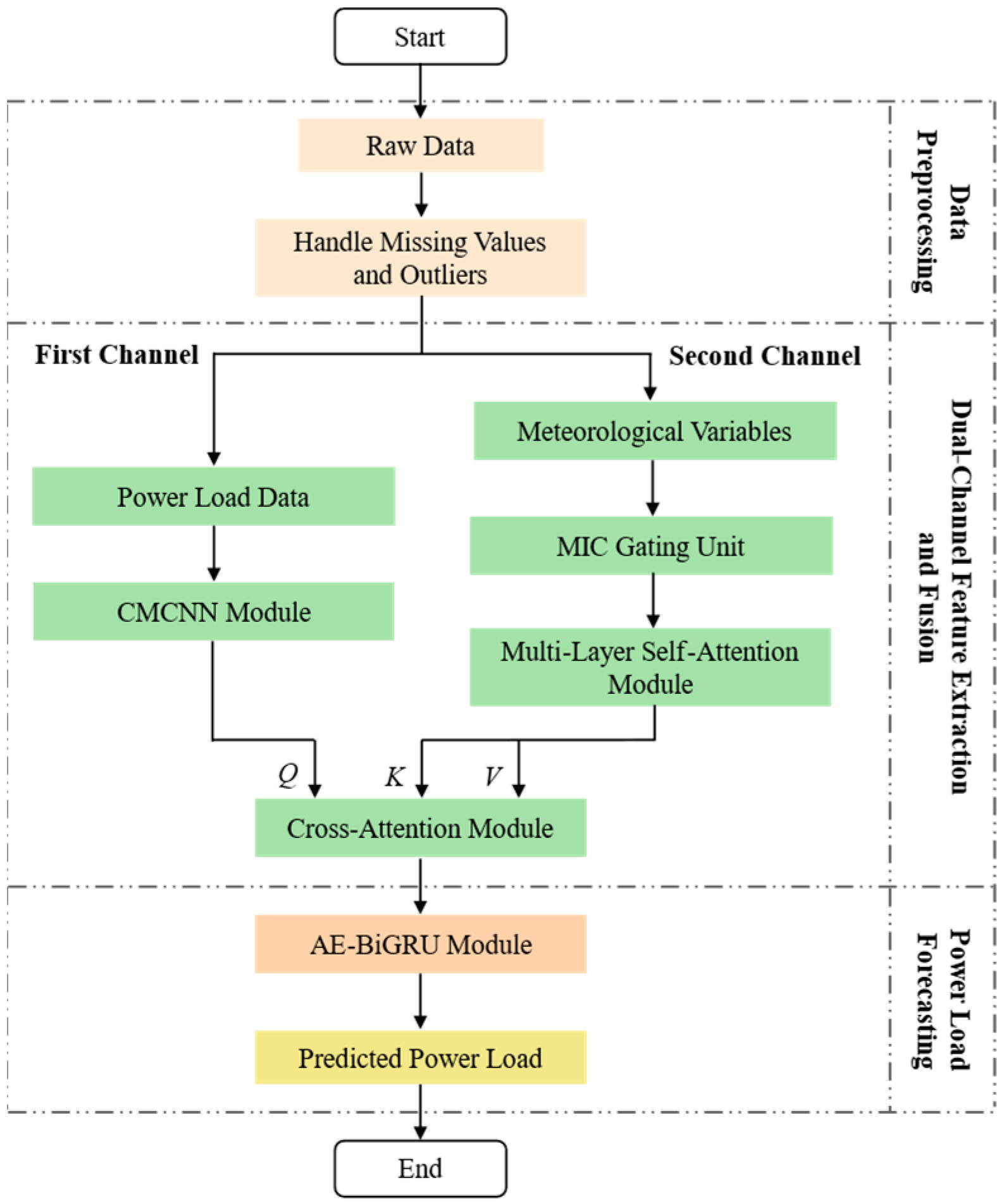
The framework of the proposed short-term power load forecasting model based on DCFE, hereafter referred to as the Main Model, is illustrated in Figure 1. It primarily consists of a data preprocessing module, a feature extraction and fusion module, and a forecasting module.

Figure 1. Framework of main model.

Because power load variations are more sensitive to meteorological factors under extreme weather, a dual-channel design is adopted in the feature extraction and fusion module to avoid the insufficient representation and mutual interference that may arise when load data and meteorological variables are simply concatenated and fed into a single-channel network. Load features and meteorological features are extracted separately. The dataset is first split into load data and meteorological variables, which serve as inputs to the two channels. In the first channel (load channel), CMCNN module is used to extract multiscale features from the load data, capturing periodicity and local fluctuations across time scales. In the second channel (meteorological channel), MIC is employed to quantify nonlinear associations between meteorological variables and power load, yielding scenario-aware prior weights. Meteorological inputs are then gated and weighted at each time step to form a weighted meteorological representation. This representation is modeled globally using a multi-layer self-attention mechanism.

Subsequently, the outputs of the two channels are dynamically fused via a cross-attention mechanism, where load features serve as the query (Q) and meteorological features serve as the key (K) and the value (V). Deep interactions between power load and meteorological factors are thus captured, yielding a more informative fused representation.

The forecasting module takes the fused features as input and performs sequence prediction using the AE-BiGRU module, producing power load forecasts for the next 24 h.

2.1. Power Load Feature Extraction with CMCNN

Power load data constitute a typical time series, and significant autocorrelation exists across time instants [28]. This dependence can be characterized by the autocorrelation coefficient c_h, whose computation is given in Equation (1):

$$c_h={\displaystyle \frac{{\displaystyle {\sum }_{i=1}^n(x_i-\overline{x})(x_{i+h}-\overline{x})}}{{\displaystyle {\sum }_{i=1}^n{(x_i-\overline{x})}^2}}}$$

(1)

Here n denotes the sequence length, h the time lag, $\overline{x}$ the mean of the load series, and x_i and x_i+h the loads at times i and i + h, respectively.

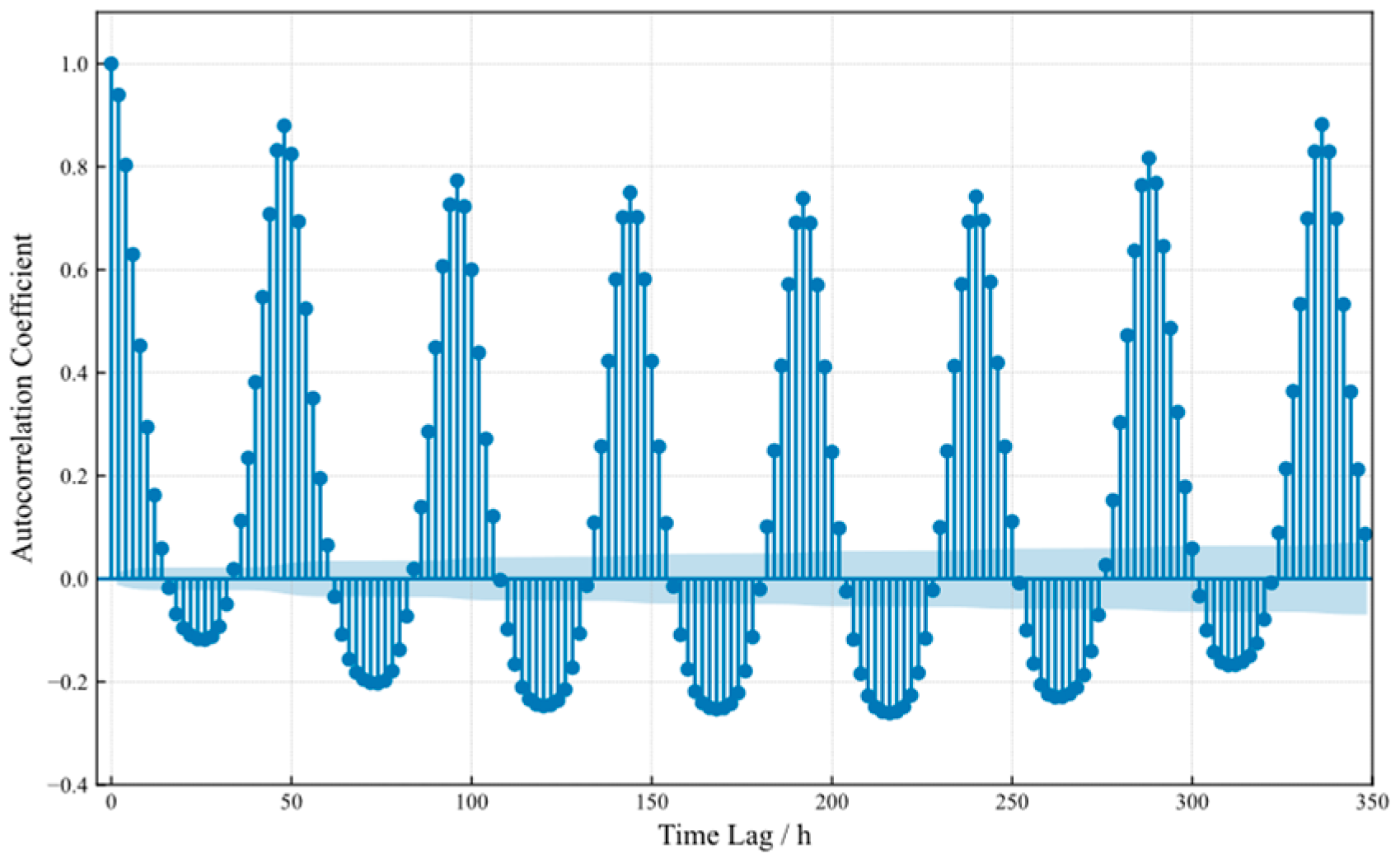
In Appendix A, Figure A1 illustrates the autocorrelation pattern of the dataset used in this study. With a sampling interval of 0.5 h, a strong positive correlation appears at a 24 h lag, whereas a moderate negative correlation is observed at a 12 h lag, indicating pronounced intraday fluctuation patterns. In addition, periodicity is observed at the weekly lag of 168 h, confirming a weekly cycle in the load.

To exploit these properties, a 7 × 48 power load input matrix X_t is constructed using a time-based sliding window method [29], as defined in Equation (2). The seven rows correspond to consecutive days and the forty-eight columns correspond to the time points within a day. This construction preserves intraday and intraweek periodicity. The window is shifted forward by 48 time points, that is, one day, to update the inputs dynamically.

$$X_t=\left[\begin{array}{cccc}{x}_t& x_{t+1}& \dots & x_{t+47}\\ x_{t+48}& x_{t+49}& \dots & x_{t+95}\\ ⋮& ⋮& \ddots & ⋮\\ x_{t+288}& x_{t+289}& \dots & x_{t+335}\end{array}\right]$$

(2)

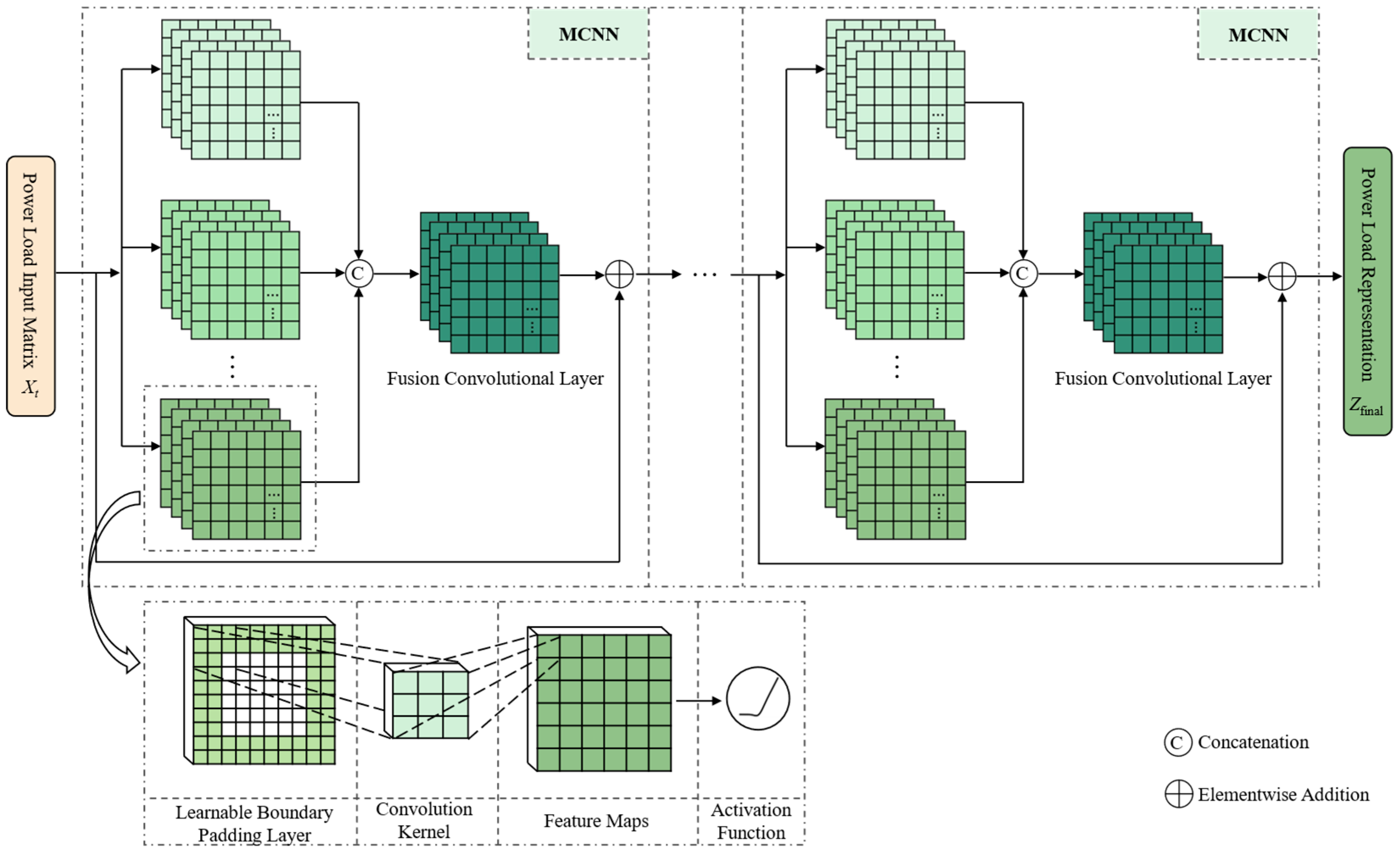
The proposed CMCNN employs multiscale two-dimensional convolutions. By designing parallel convolutional kernels at multiple scales, the receptive field is effectively expanded and the modeling of global dependencies is enhanced. Two-dimensional kernels capture intraday local features along the column dimension and cross day global periodic trends along the row dimension. The feature extraction mechanism of 2D CNN aligns with the construction of X_t, which facilitates effective extraction of both local and periodic information.

Figure 2 presents the overall structure of the CMCNN module. The network consists of multiple multiscale convolutional module (MCNN) connected in series. Each MCNN contains several parallel two-dimensional branches with different kernel sizes to extract features of the load across multiple time scales. The input is first processed with learnable boundary padding to strengthen the representation of edge regions. Feature maps from the branches are passed through the GELU activation [30], concatenated along the channel dimension, and then integrated by a fusion convolutional layer, yielding the power load representation Z_final.

Figure 2. Structure of CMCNN module.

2.1.1. Learnable Boundary Padding Layer

In convolution operations, maintaining consistent shapes between the input and the output is critical to ensuring accurate extraction of temporal patterns. This consistency is particularly important when modeling cyclical variations and complex weather-induced power load fluctuations, as it ensures that convolution kernels cover the entire input and prevents omission of edge features. However, traditional zero padding methods, while resolving shape consistency, introduce fixed values at the boundaries. These values fail to reflect the true distribution of the input data, potentially reducing the accuracy of edge representation and impairing the integrity of overall feature extraction.

To address this issue, a learnable boundary padding layer is proposed. This layer adaptively adjusts the size of the padding region according to kernel dimensions. The required numbers of rows and columns to be padded are determined by the kernel height and width, as defined in Equation (3).

$$\left\{\begin{array}{l}\mathrm{padding}\text{\_}\mathrm{top}=⌊{\displaystyle \frac{K_h-1}{2}}⌋\\ \mathrm{padding}\text{\_}\mathrm{bottom}=K_h-1-\mathrm{padding}\text{\_}\mathrm{top}\\ \mathrm{padding}\text{\_}\mathrm{left}=⌊{\displaystyle \frac{K_w-1}{2}}⌋\\ \mathrm{padding}\text{\_}\mathrm{right}=K_w-1-\mathrm{padding}\text{\_}\mathrm{left}\end{array}\right.$$

(3)

Here, K_h and K_w denote the kernel height and width, respectively. Through adaptive learning, the padding values are treated as trainable parameters and updated during backpropagation, ensuring that the padded region better approximates the true distribution of power load data. This mechanism not only avoids the loss of edge features but also enhances the adaptability of the model under multiple weather scenarios and cyclical load fluctuations.

2.1.2. MCNN Module

Unlike conventional CNN architectures, the MCNN module introduces parallel convolutions at multiple scales, enhancing feature modeling of power load across different temporal granularities. Larger kernels are used to extract global trend characteristics, such as daily and weekly periodicity, whereas smaller kernels focus on short-term local fluctuations, thereby providing complementary representations of global trends and local variations.

To further improve representational hierarchy and richness, multiple MCNNs are connected in series to form a hierarchical feature extraction architecture. Each module refines and enriches global and local characteristics based on the features from the previous layer through cascading, yielding deeper feature representations. The combination of serial connection and cascading overcomes the limitations of a single convolutional block and enables progressive distillation of complex dynamics in the load data. In addition, residual connections are incorporated within the module to stabilize deep training. By adding the input features to the convolutional output, stable feature propagation is ensured and gradient attenuation is mitigated.

2.2. Meteorological Feature Extraction with Multi-Layer Self-Attention

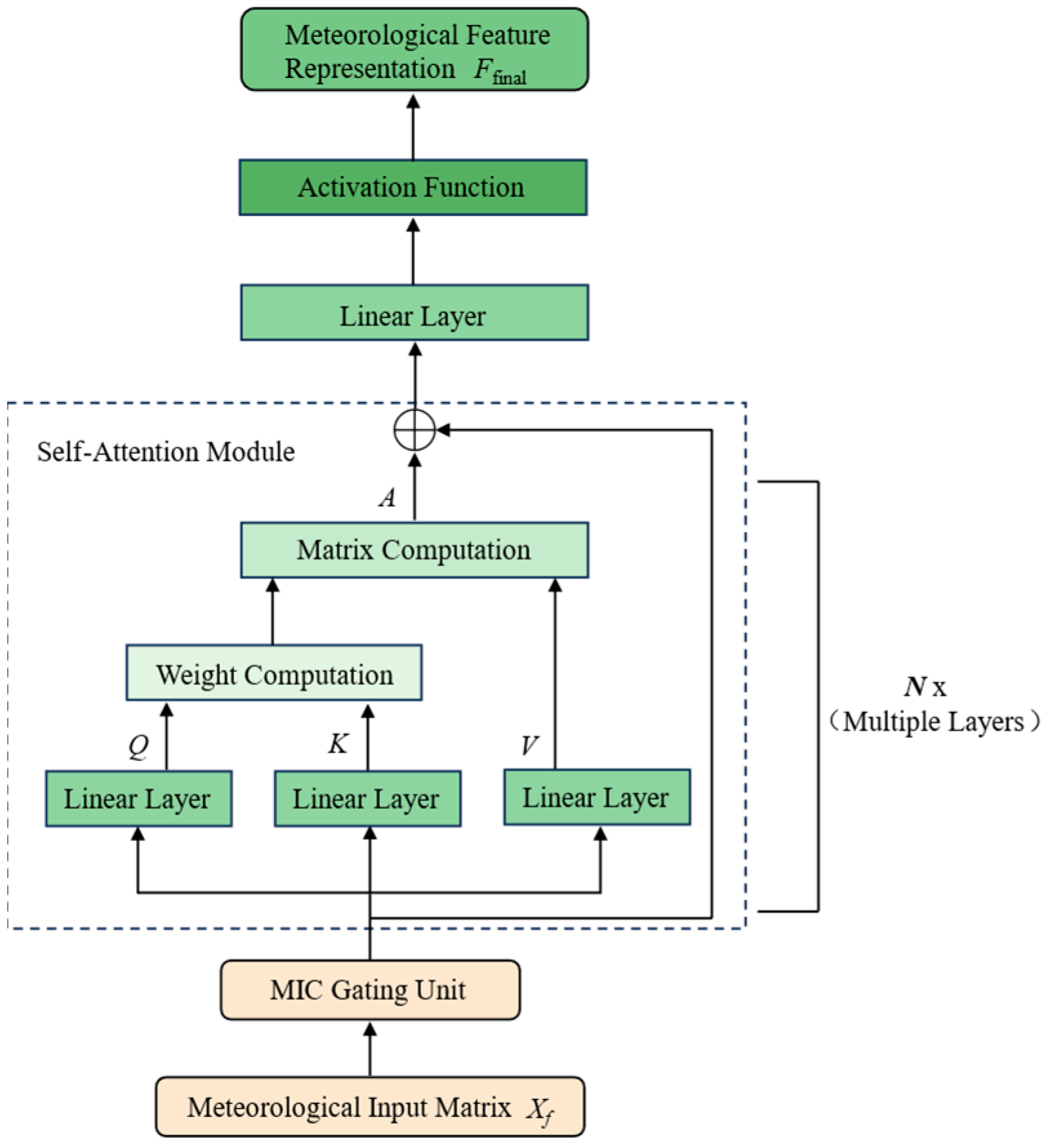
The second channel consists of an MIC gating unit and multiple serial self-attention modules, as illustrated in Figure 3.

Figure 3. Structure of the multi-layer self-attention model.

Because correlations between power load and meteorology vary significantly across weather scenarios, directly inputting meteorological data or applying globally shared weights may weaken the generalization capability across scenarios. To address this, before entering the self-attention modules, the meteorological input matrix X_f $\in {ℝ}^{L\times F}$ (where F is the number of meteorological variables and L the sequence length) is processed by a scenario-based MIC gating unit. This unit adaptively adjusts the weights of variables across scenarios, enabling selective emphasis on scenario-relevant signals, suppressing weakly correlated variables, and enhancing the ability of subsequent self-attention to discriminate key meteorological drivers.

The MIC gating unit first determines the weather scenario s_t at each time step according to the weather type definition. Given a fixed scenario s and meteorological variable f, the MIC is computed on the training set to measure the nonlinear association between the variable sequence X_f and the power load Y. The resulting prior weight m_s,f is defined as follows:

$$m_{s,f}=\underset{G_x,G_y}{\max }{\displaystyle \frac{I_s(X_f,Y;G_x,G_y)}{\log \min (G_x,G_y)}}$$

(4)

$$I_s(X_f,Y;G_x,G_y)={\displaystyle \sum _{i=1}^{\left|G_x\right|}{\displaystyle \sum _{j=1}^{\left|G_y\right|}{p}_{ij}^{(s)}\log \frac{p_{ij}^{(s)}}{p_{i\cdot }^{(s)}{p}_{\cdot j}^{(s)}}}}$$

(5)

where |G_x| and |G_y| denote the numbers of grid partitions for X_f and Y, respectively; $p_{ij}^{(s)}$ is the joint probability that the pair falls into cell (i, j) under scenario s; and $p_{i\cdot }^{(s)}$, $p_{\cdot j}^{(s)}$ are the corresponding marginal probabilities.

The prior weight m_s,f is then sharpened by a power operation to enhance separation between strong and weak correlations and normalized across variables. The resulting gating weight g_s,f ϵ [0, 1] for variable f under scenario s is given by:

$${\tilde{m}}_{s,f}={(m_{s,f}+\epsilon )}^{\gamma }$$

(6)

$$g_{s,f}={\displaystyle \frac{{\tilde{m}}_{s,f}}{{\displaystyle {\sum }_{f^{\prime }}{\tilde{m}}_{s,f^{\prime }}}}}$$

(7)

where ε > 0 is a numerical stability constant (e.g., 10⁻⁸), and γ > 1 is the sharpening exponent.

Finally, each meteorological variable x_t,f is weighted elementwise by $g_{s_t,f}$, yielding the following gated result:

$${\widehat{x}}_{t,f}=g_{s_t,f}\odot x_{t,f}$$

(8)

where ⊙ denotes the elementwise (Hadamard) product.

The gated meteorological sequence ${\widehat{X}}_f$ is processed in order by self-attention, a linear layer, and an activation function, and a residual connection is employed to ensure effective information propagation. After layer wise processing by multiple modules, the meteorological feature representation F_final is produced for subsequent feature fusion.

Within self-attention, the input matrix is linearly projected to obtain the query matrix Q, key matrix K, and value matrix V for computing pairwise dependencies within the sequence, as shown in Equation (9):

$$\left\{\begin{array}{c}{Q}^{(l)}={\widehat{X}}_f^{(l)}{W}_Q^{(l)}\\ K^{(l)}={\widehat{X}}_f^{(l)}{W}_K^{(l)}\\ V^{(l)}={\widehat{X}}_f^{(l)}{W}_V^{(l)}\end{array}\right.$$

(9)

Here Q^(l), K^(l), and V^(l) denote the query, key, and value at the l-th self-attention module, and $W_Q^{(l)},W_K^{(l)},W_V^{(l)}$ are the corresponding projection matrices.

Next, the attention weights are computed via the dot product between Q and K, followed by multiplication with V to produce the following attention output:

$$\begin{array}{c}{\mathrm{A}}^{(l)}(Q^{(l)},K^{(l)},V^{(l)})=\\ softmax({\displaystyle \frac{Q^{(l)}{K}^{{(l)}^T}}{\sqrt{F}}})V^{(l)}\end{array}$$

(10)

2.3. Feature Fusion with Cross-Attention

Within the dual-channel feature extraction framework, load features and meteorological variables are modeled in independent channels. To achieve effective feature level integration, a cross-attention-based feature fusion module is introduced. The computation of the feature fusion module follows Equations (9) and (10). Its structure is consistent with Figure 3, while the inputs and outputs differ, and the MIC gating unit is not included.

The output of the load channel Z_final is linearly projected to the query matrix Q. The output of the meteorological channel F_final is projected to the key matrix K and the value matrix V. Attention weights are computed along the daily dimension and used to linearly weight V, yielding the fused feature representation T_final, which provides a more comprehensive input for subsequent power load forecasting.

Scenario-specific dynamic weighting has already been applied by MIC gating in the upstream meteorological channel. Cross-attention further performs cross-source alignment at a daily granularity level and achieves attention guided aggregation, so that the attention distribution aligns with scenario-relevant variables. This facilitates the capture of complex variation patterns and provides a more reliable basis for accurate forecasting.

3. Power Load Forecasting with AE-BiGRU

3.1. Architecture of AE-BiGRU

Under extreme weather scenarios, power load exhibits stronger randomness and contingency, which increases the difficulty of forecasting. To more effectively capture temporal dependencies in the fused features and to improve performance across multiple weather scenarios, the AE-BiGRU model is proposed. The model combines a bidirectional GRU with an attention enhancement mechanism, enabling dynamic focus on salient sequence characteristics and effective representation of complex load patterns under both normal and extreme weather.

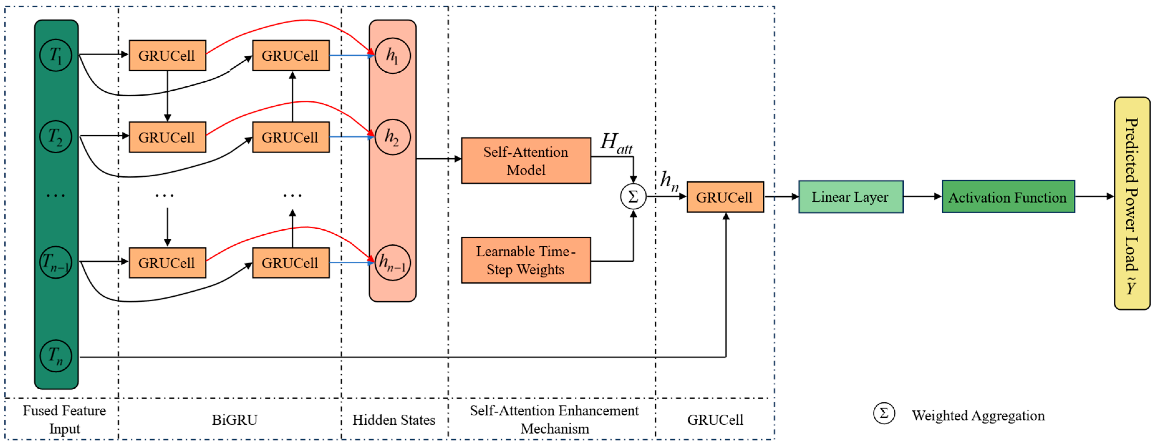
Figure 4 presents the overall structure of the AE-BiGRU module. The fused feature sequence T₁ to T_n−1 is first fed into the BiGRU block, where bidirectional GRU cells extract contextual hidden states at each time step. These hidden states are then processed by a self-attention module to refine global temporal features, and learnable time-step weights are applied to perform weighted aggregation of the sequence representation. The aggregated representation h_n together with the last time step input T_n is provided to a GRU cell to further refine fine grained characteristics. Finally, the output is passed through a linear layer and an activation function to produce the predicted power load $\tilde{Y}$.

Figure 4. Structure of AE-BiGRU module.

3.2. Bidirectional Gated Recurrent Unit

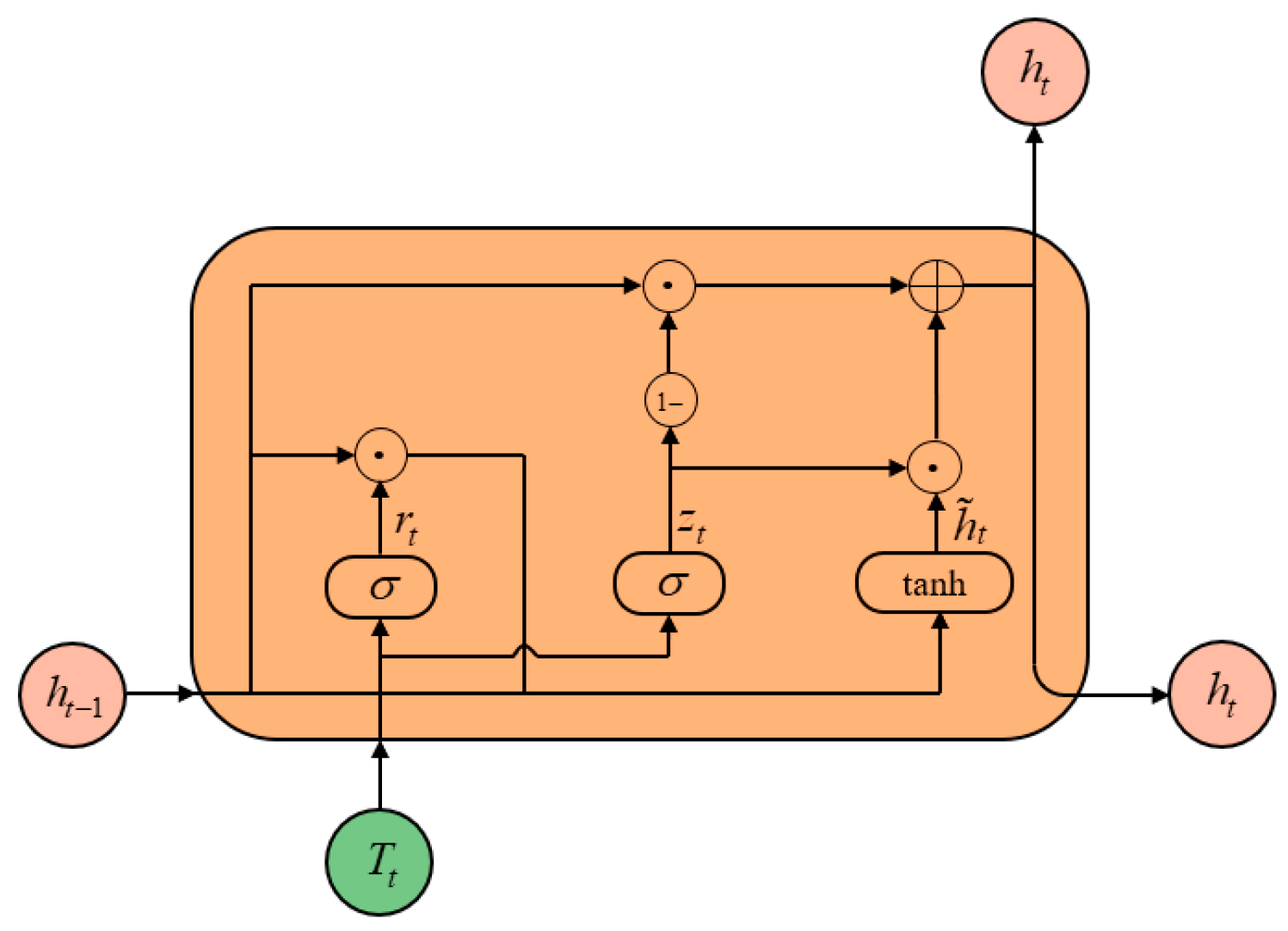
The BiGRU is a neural architecture commonly used for time series modeling. Compared with conventional recurrent networks, the GRU alleviates vanishing and exploding gradients through gating mechanisms. Building on this idea, the BiGRU adopts a bidirectional structure that exploits both forward and backward context, thereby enhancing the modeling of complex temporal patterns [31], as illustrated in Appendix A, Figure A2.

The BiGRU output at time t is given as follows:

(1)

Forward computation:

$$\left\{\begin{array}{l}{\overrightarrow{z}}_t=\sigma ({\overrightarrow{W}}_z{T}_t+{\overrightarrow{U}}_z{\overrightarrow{h}}_{t-1}+{\overrightarrow{b}}_z)\\ {\overrightarrow{r}}_t=\sigma ({\overrightarrow{W}}_r{T}_t+{\overrightarrow{U}}_r{\overrightarrow{h}}_{t-1}+{\overrightarrow{b}}_r)\\ {\overrightarrow{\tilde{h}}}_t=\tanh [{\overrightarrow{W}}_h{T}_t+{\overrightarrow{U}}_h({\overrightarrow{r}}_t\odot {\overrightarrow{h}}_{t-1})+{\overrightarrow{b}}_h]\\ {\overrightarrow{h}}_t=(1-{\overrightarrow{z}}_t)\odot {\overrightarrow{h}}_{t-1}+{\overrightarrow{z}}_t\odot {\overrightarrow{\tilde{h}}}_t\end{array}\right.$$

(11)

(2)

Backward computation:

$$\left\{\begin{array}{l}{\overleftarrow{z}}_t=\sigma ({\overleftarrow{W}}_z{T}_t+{\overleftarrow{U}}_z{\overleftarrow{h}}_{t+1}+{\overleftarrow{b}}_z)\\ {\overleftarrow{r}}_t=\sigma ({\overleftarrow{W}}_r{T}_t+{\overleftarrow{U}}_r{\overleftarrow{h}}_{t+1}+{\overleftarrow{b}}_r)\\ {\overleftarrow{\tilde{h}}}_t=\tanh [{\overleftarrow{W}}_h{T}_t+{\overleftarrow{U}}_h({\overleftarrow{r}}_t\odot {\overleftarrow{h}}_{t+1})+{\overleftarrow{b}}_h]\\ {\overleftarrow{h}}_t=(1-{\overleftarrow{z}}_t)\odot {\overleftarrow{h}}_{t+1}+{\overleftarrow{z}}_t\odot {\overleftarrow{\tilde{h}}}_t\end{array}\right.$$

(12)

Here → and ← denote forward and backward directions, T_t and h_t denote the input and the hidden state at time t, $\sigma$ is the sigmoid activation, tanh is the hyperbolic tangent, r_t and z_t are the reset and update gates, ${\tilde{h}}_t$ is the candidate hidden state, W_r, W_z, W_h, U_r, U_z, and U_h are weight matrices, and b_r, b_z, and b_h are bias terms.

3.3. Self-Attention Enhancement Mechanism

Although the BiGRU is advantageous for capturing historical temporal information, earlier information diminishes as the sequence length increases, which causes dilution of some critical signals during propagation. To alleviate this issue, a self-attention enhancement mechanism is embedded within the conventional BiGRU to dynamically allocate feature weights across time, thereby improving forecasting performance.

Specifically, the self-attention enhancement mechanism takes the hidden states from the first n − 1-time steps as input and produces a weighted representation, H_att, through a self-attention module. Conventional self-attention assigns weights based on pairwise similarity across time steps, which can lead to over averaging and may overlook contributions from important time points. Therefore, learnable time step weights are introduced to adaptively optimize the contribution of each time step, enabling dynamic adjustment of temporal importance and more effective capture of features critical to power load forecasting. Finally, the representation H_att is aggregated with time step weights to obtain the history-informed composite representation h_n:

$$h_n={\displaystyle \sum _{i=1}^{n-1}{w}_{\mathrm{time},i}\cdot H_{\mathrm{att},i}}$$

(13)

Here w_time,i denotes the learnable weight for time step i, and H_att,i denotes the attention-processed representation at time step i.

4. Case Study Analysis

4.1. Case Description

The dataset comprises aggregated residential and commercial power loads from a region in Australia, spanning October 2018 to October 2023, with a sampling interval of 30 min that yields 48 load time points per day. The dataset includes power loads and four meteorological variables; detailed feature descriptions are provided in Appendix A, Table A1. The data were partitioned into 80% for training, 10% for validation, and 10% for testing. The forecasting horizon was set to one day, that is, the model output power load predictions for the next 48 time points.

4.1.1. Data Preprocessing

Because data loss and anomalies may occur during acquisition or transmission, missing values and outliers must be addressed. Two procedures were adopted to ensure data completeness and validity. First, missing values were imputed using a decision tree regressor, which inferred missing entries from other features and improved consistency. Second, outliers were detected by a Local Outlier Factor (LOF) algorithm [32] and replaced using the decision tree model. To remove scale differences across features, standardization was applied so that features shared a comparable distribution. The standardization formula is given as follows.

$$X_{\mathrm{norm}}={\displaystyle \frac{X-\mu }{s}}$$

(14)

Here X denotes the raw value, $\mu$, the feature mean, and s, the feature standard deviation.

4.1.2. Evaluation Metrics

To evaluate the forecasting performance of the model, five commonly used metrics were employed: Mean Absolute Error (MAE), Mean Absolute Percentage Error (MAPE), Root Mean Square Error (RMSE), Symmetric Mean Absolute Percentage Error (sMAPE), and the coefficient of determination (R²). The formulas for these evaluation metrics are given as follows.

$$\mathrm{MAE}={\displaystyle \frac{1}{n}}{\displaystyle \sum _{i=1}^n\left|{\tilde{y}}_i-y_i\right|}$$

(15)

$$\mathrm{MAPE}={\displaystyle \frac{100\%}{n}}{\displaystyle \sum _{i=1}^n\left|\frac{{\tilde{y}}_i-y_i}{y_i}\right|}$$

(16)

$$\mathrm{RMSE}=\sqrt{{\displaystyle \frac{1}{n}}{\displaystyle \sum _{i=1}^n{({\tilde{y}}_i-y_i)}^2}}$$

(17)

$$\mathrm{sMAPE}={\displaystyle \frac{100\%}{n}}{\displaystyle \sum _{i=1}^n\frac{\left|{\tilde{y}}_i-y_i\right|}{(\left|{\tilde{y}}_i\right|+\left|y_i\right|)/2}}$$

(18)

$$R^2=1-{\displaystyle \frac{{\displaystyle {\sum }_{i=1}^n{({\tilde{y}}_i-y_i)}^2}}{{\displaystyle {\sum }_{i=1}^n{(y_i-\overline{y})}^2}}}$$

(19)

Here n denotes the number of forecasting samples; $\tilde{Y}=[{\tilde{y}}_1,{\tilde{y}}_2,\dots ,{\tilde{y}}_n]$, the predicted value; $Y=[y_1,y_2,\dots ,y_n]$, the actual value; and $\overline{y}$, the mean of the actual values.

4.1.3. Hyperparameter Settings

Hyperparameters for the main model, baseline models, and ablation variants were tuned within the Optuna framework using a Bayesian optimization strategy, enabling automated search and ensuring fairness and rigor in performance comparison. Detailed configurations of the main model are provided in Appendix A, Table A2.

4.2. Analysis of Relative Importance of Meteorological Variables

Based on the quantile thresholds in Table 1, the weather scenario was determined at each time step, and historical samples were partitioned into normal, high-temperature, low-temperature, high humidity, and hot humid conditions. Within each scenario, the MIC was used to measure the nonlinear association between meteorological variables and power load. As shown in Table 2, the dry bulb temperature exhibits a higher correlation with MIC under normal weather; dry bulb and wet bulb temperature correlations with MICs are particularly prominent under high- and low-temperature scenarios; dew point, relative humidity, and wet bulb temperature correlations with MICs become more pronounced under high humidity; and all four variables show strong correlations under hot humid conditions. These differences indicate the need to incorporate scenario dependence into the weighting of meteorological features.

Table 1. Definitions of adverse weather conditions.

Adverse Weather	Definition	Note
High Temperature	T > Quantile0.99 (Dry Bulb Temperature)	Quantile0.99 (Dry Bulb Temperature) denotes the 99th percentile of dry bulb temperature.
Low Temperature	T < Quantile0.01 (Dry Bulb Temperature)	Quantile0.01 (Dry Bulb Temperature) denotes the 1st percentile of dry bulb temperature.
High Humidity	H > Quantile0.99 (Humidity)	Quantile0.99 (Humidity) denotes the 99th percentile of relative humidity.
Hot Humid	T > Quantile0.95 (Wet Bulb Temperature) and H > Quantile0.95 (Humidity)	Quantile0.95 (Wet Bulb Temperature) denotes the 95th percentile of wet bulb temperature.

Table 2. Analysis results of MIC.

Meteorological Feature	MIC
	Normal	High Temperature	Low Temperature	High Humidity	Hot Humid
Dry Bulb Temperature	0.41	0.60	0.54	0.38	0.49
Dew Point Temperature	0.36	0.39	0.36	0.47	0.51
Wet Bulb Temperature	0.29	0.58	0.52	0.50	0.58
Relative Humidity	0.26	0.33	0.26	0.62	0.58

To quantify the relative importance of variables on a common scale within the same time step, a relative weight was constructed from the MIC based gating weight and the meteorological value x_t,f.

$$\mathrm{share}(t,f)={\displaystyle \frac{g_{s_t,f}\left|x_{t,f}\right|}{{\displaystyle {\sum }_{f^{\prime }}{g}_{s_t,f^{\prime }}\left|x_{t,f^{\prime }}\right|}}}$$

(20)

Here |x_t,f| denotes the magnitude of variable f at time t with absolute value taken to remove sign effects.

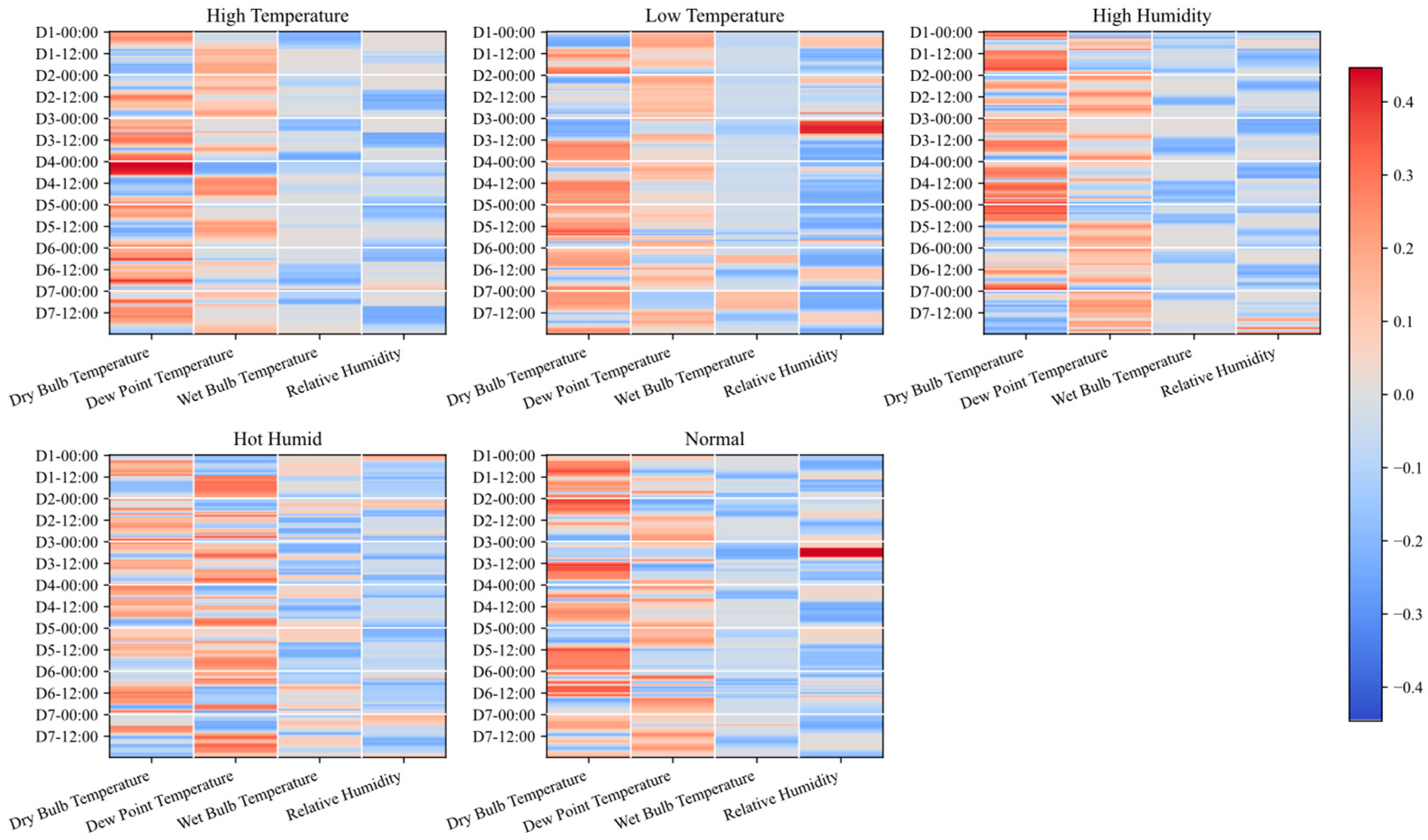
To align with scenario-based forecasting experiments, samples were grouped by the scenario label of the target day. The preceding seven days served only as the observation window for that group, and their weather types were unrestricted. Appendix A, Figure A3 presents the distributions of relative weights for each variable within groups over the seven-day window prior to the target day, together with their evolution across time steps. To visualize deviations from a uniform baseline, where the four variables each account for one quarter, the color scale encodes (t, f)-1/4. Red indicates values above the baseline, that is, relative emphasis; blue indicates values below the baseline, that is, relative suppression; near white indicates an approximately uniform allocation.

Based on these observations, MIC gating, compared with static weights, adaptively adjusts variable weights across scenarios and time steps. It dynamically emphasizes meteorological variables that are more relevant to the current load state and suppresses weakly related ones, which avoids correlation mismatch and injection of irrelevant information during scenario transitions. Consequently, cross channel fusion becomes more selective and consistent, and the robustness of fusion is improved.

4.3. Analysis of Forecasting Results

4.3.1. Comparative Experiments

Under different weather conditions, the power load exhibits pronounced physical differences. Extremely high temperatures sustain heavy operation of cooling equipment and lift daytime peaks. Low temperatures increase demand for heating and water heating, leading to steep rises at night and in the early morning. High humidity intensifies dehumidification and ventilation, which prolongs the post peak decline. In hot humid scenarios, the combined effects of temperature and humidity yield more complex multi peak and nonlinear fluctuations in the load curve. These sensible heat- and latent-heat-driven processes make forecasting under extreme weather more challenging.

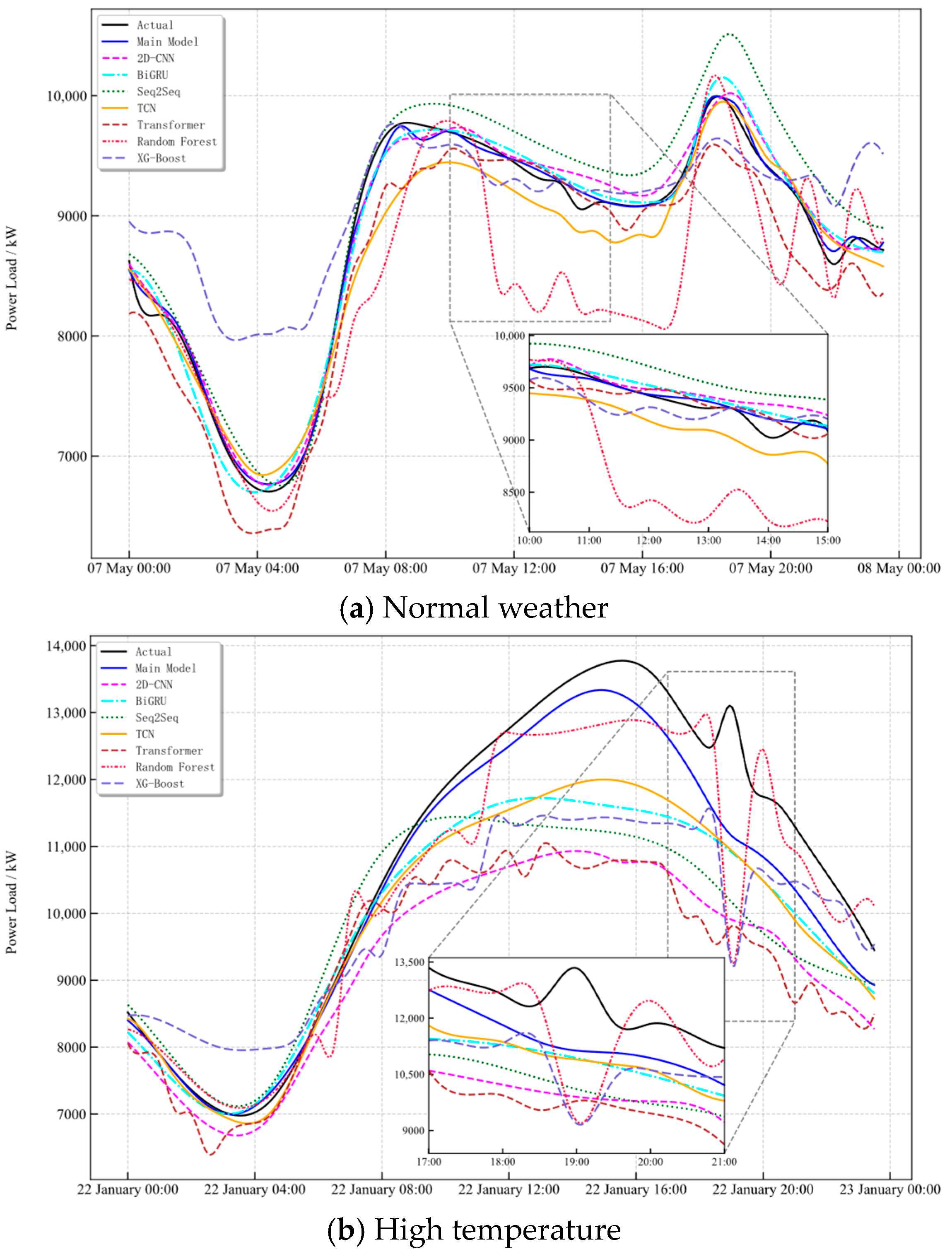
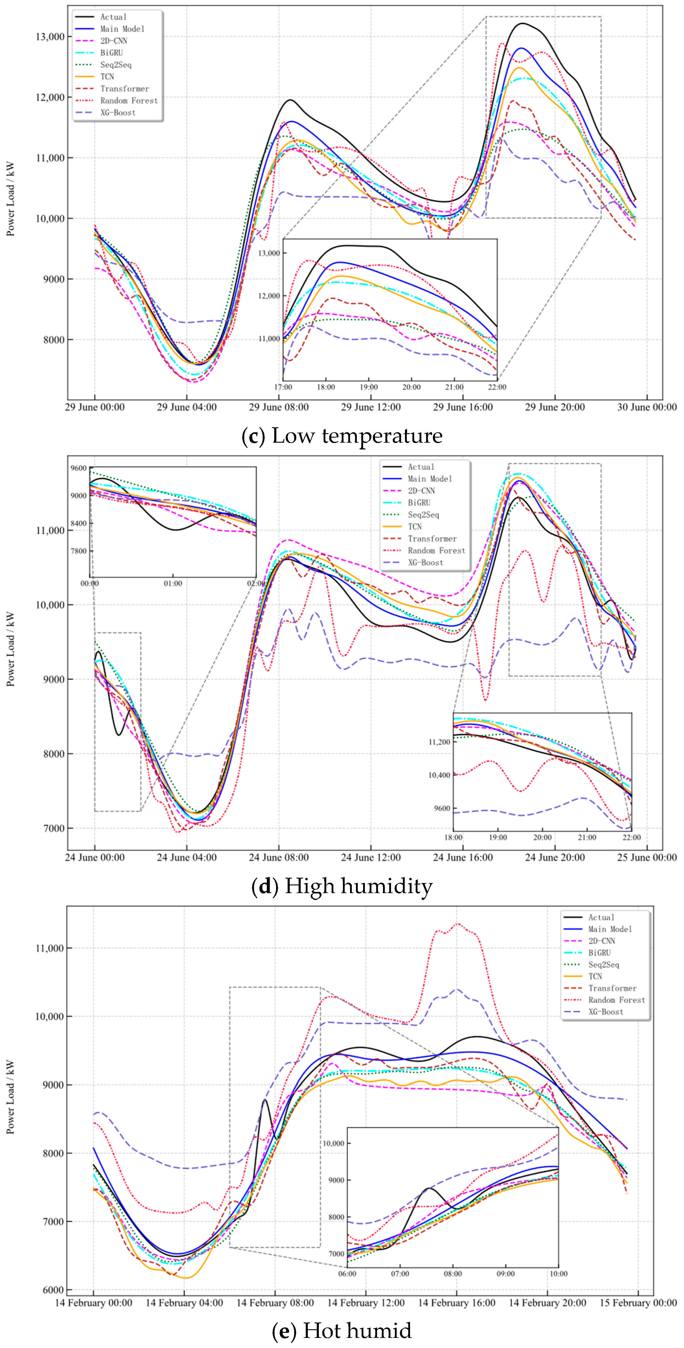
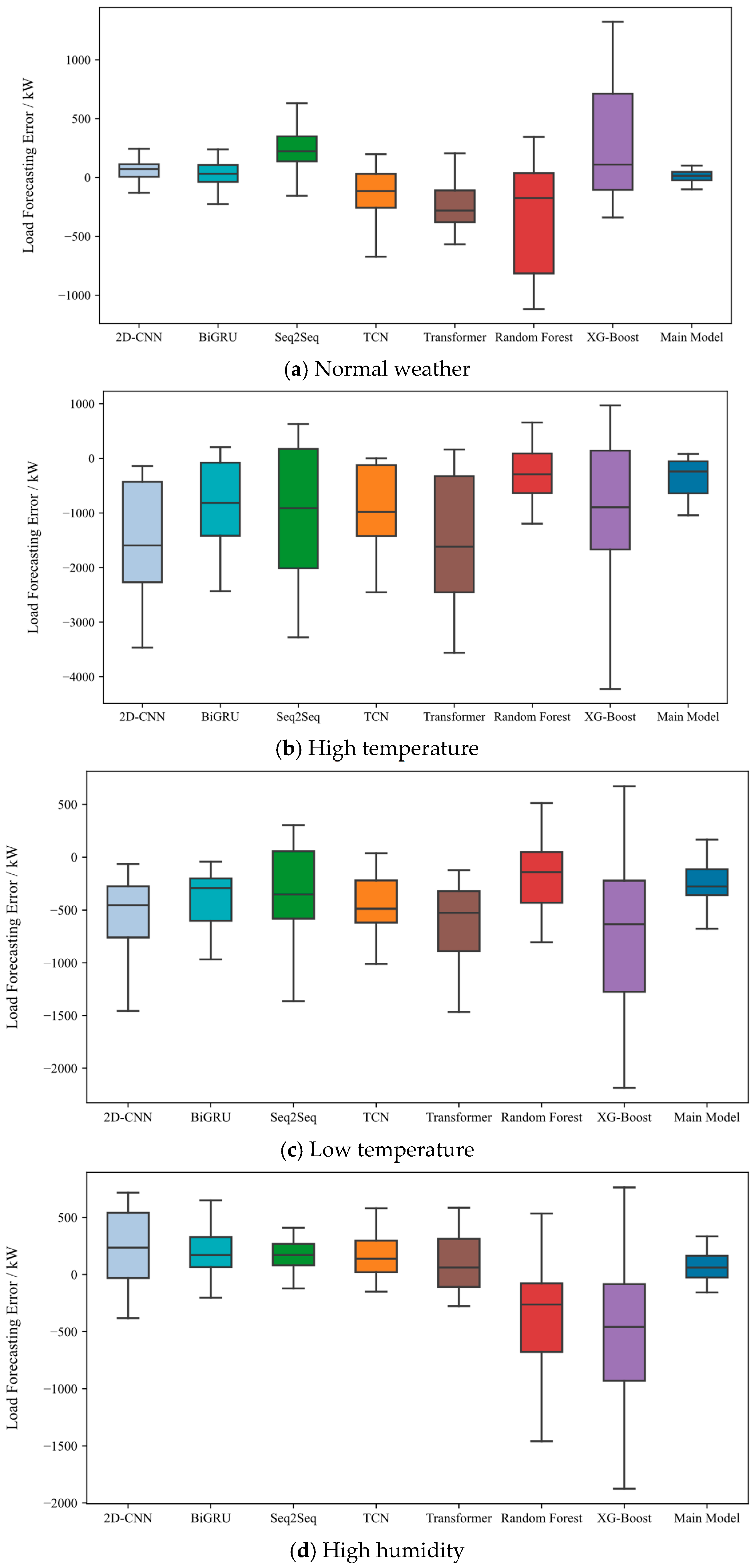
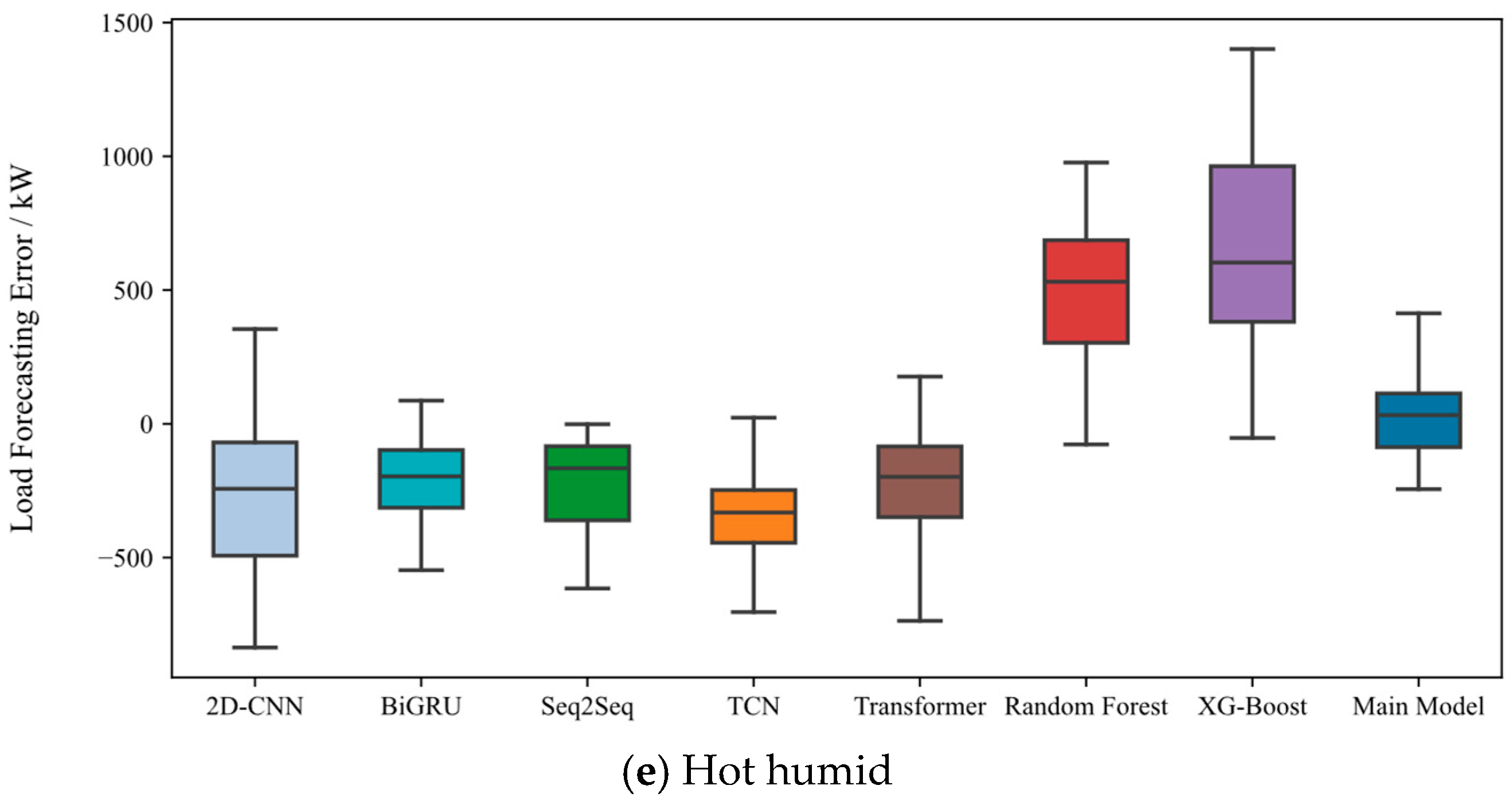
Against this background, a series of experiments covering typical weather scenarios—including normal, high-temperature, low-temperature, high humidity, and hot humid conditions—were designed to systematically evaluate the adaptability and robustness of the proposed model under diverse weather conditions. The prediction results of all primary and baseline models, including 2D-CNN, BiGRU, Seq2Seq, TCN, Transformer, Random Forest, and XG-Boost, were inverse standardized to ensure comparability of scales with the measured load. For each weather category, one day was randomly selected as a test sample. The waveform comparisons and error box plots are shown in Figure 5 and Figure 6.

Figure 5. Comparison of prediction curves for different baseline models.

Figure 6. Box plot of prediction errors for different models.

Under normal weather conditions, the main model accurately captures the entire trough–peak–recession pattern, including the peak timing, amplitude, and plateau-to-decline rhythm, while maintaining stable tracking of minor post-noon fluctuations. Most baseline models exhibit overall negative bias during and after the peak period. XG-Boost shows larger afternoon dispersion, while Random Forest demonstrates pronounced underestimation accompanied by oscillations. The boxplot analysis indicates that the proposed model yields residuals with a near-zero median and the smallest interquartile range, demonstrating the best overall robustness.

In the high-temperature sample, the arrival time and magnitude of the main peak are well captured. The rapid rise before the peak is fitted well, and only slight deviations appear in the post peak decline, while the overall trend remains consistent. The waveform and box plots indicate that the baselines exhibit negative bias with long tails around the peak segment, whereas the proposed model shows more concentrated residuals. In the low-temperature sample, both morning and evening contain valley-to-peak rises. Most baselines display overall negative residuals during these periods, while the proposed model yields more concentrated errors.

In the high humidity sample, the main model’s behavior in the transition between the primary and secondary peaks and in the post peak recession is particularly sensitive to humidity-driven persistence and the rhythm of information decay. Zoomed-in views further reveal slightly weaker tracking of fine-scale undulations during the 00:00–02:00 trough-to-rise stage and enlarged deviations at specific intervals within the 18:00–22:00 evening peak-to-valley recession, manifesting as mild phase shifts and amplitude offsets.

In the hot humid sample, the superposition of temperature and humidity makes peak elevation and transition asymmetry more pronounced. The proposed model aligns well with the measurements in peak timing, amplitude, and transition slope, whereas some baselines present opposite bias around the peak and transition segments, and their box plots display elongated upper and lower spreads.

Across the five weather scenarios, all five metrics in Appendix A, Table A3 improve overall, which is consistent with the observed waveform and residual distribution changes. This performance advantage is primarily attributed to the synergy between the dual-channel architecture and the AE-BiGRU design. Scenario-based MIC dynamic weighting highlights key variables within the meteorological channel, thereby emphasizing the drivers in high- and low-temperature scenarios. Meanwhile, cross-attention at a daily granularity level aligns and fuses load and meteorological representations. Together with the learnable time step weights in AE-BiGRU, key historical periods are emphasized, which yields more robust characterization of peak timing, amplitude, and slope under extreme and nonstationary meteorological conditions.

4.3.2. Visualization of the Feature Fusion Module

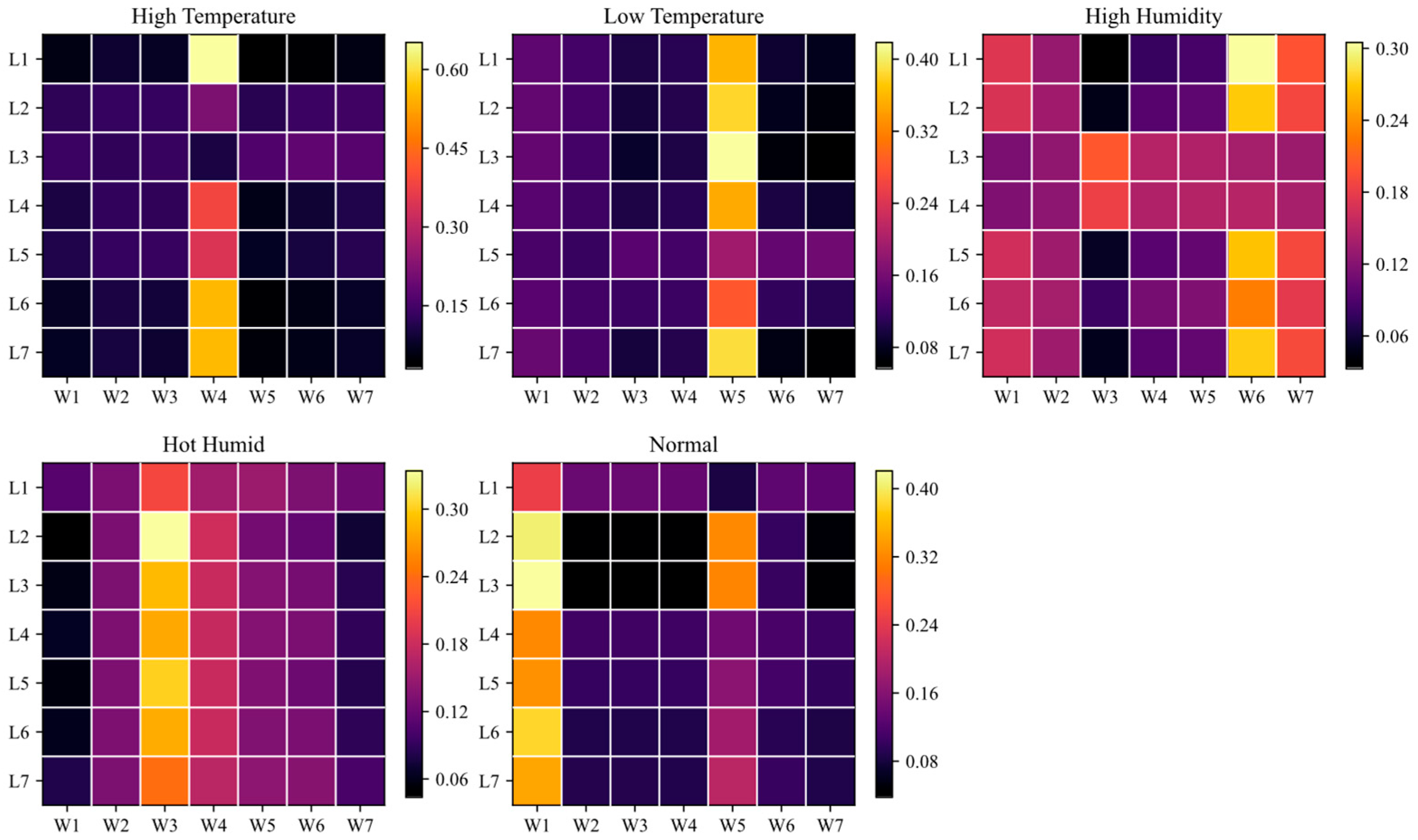
Building on the quantitative results above, attention heat maps of the feature fusion module are provided to reveal cross channel attention allocation during fusion, as shown in Appendix A, Figure A4. The horizontal axis, W1 to W7, represents meteorological representations from the meteorological channel for the seven days prior to the target day. The vertical axis, L1 to L7, represents power load representations from the load channel for the corresponding seven historical days.

The heat maps show that attention concentrates on a few key meteorological days in a manner consistent with the weather scenario, and the temporal pattern largely echoes the relative weight distributions in Appendix A, Figure A3. In the high-temperature scenario, column W4 carries larger weights across many rows, which aligns with the dominance of dry bulb temperature around day D4 in Figure A3. In the low-temperature scenario, attention concentrates on W5, consistent with the high dry bulb temperature at D5. In the high humidity scenario, attention mainly falls on W6 and extends to W7 for a subset of samples, which agrees with the persistently elevated dew points and relative humidities on adjacent days in Figure A3. In the hot humid scenario, attention concentrates on W3 and W4, matching the jointly high dry bulb temperatures and dew points on the corresponding days. In the normal weather scenario, attention is primarily concentrated in columns W1 and W5, corresponding to the high-weight regions of dry bulb temperature at periods D1 and D5 in Figure A4.

Overall, the fusion module preferentially allocates attention from the load side to more discriminative meteorological day representations. The temporal distribution of attention is broadly consistent with the scenario-specific variable weights characterized by MIC gating. By comparing Figure A3 and Figure A4, a clear correspondence is established between the variable-level and the day-level associations, which delineates information selection and cross-source alignment under extreme weather and enhances model interpretability.

4.4. Ablation Study

To investigate the specific impact of each module on overall performance, ablation experiments were designed, where selected components were adjusted or removed to evaluate their contributions to forecasting accuracy and robustness. The experiments were intended to validate the rationality of the main architecture and to clarify the practical contribution of each module through comparisons across model configurations. The ablation settings were aligned with Section 4.3 and were evaluated on the same dataset. Table 3 provides the configurations of the ablation variants.

Table 3. Description of ablation models.

Model	Description
Model 1	Dual-channel design removed. CMCNN is used with load data and meteorological features jointly as inputs.
Model 2	Self-attention enhancement module in AE BiGRU removed.
Model 3	Feature fusion module removed. Outputs from the two channels are concatenated and fed directly to AE-BiGRU.
Model 4	Learnable padding in CMCNN removed. Convolution kernel size fixed to (3, 3).
Model 5	MIC gating unit removed. Meteorological variables are fed to the second channel without dynamic weighting.

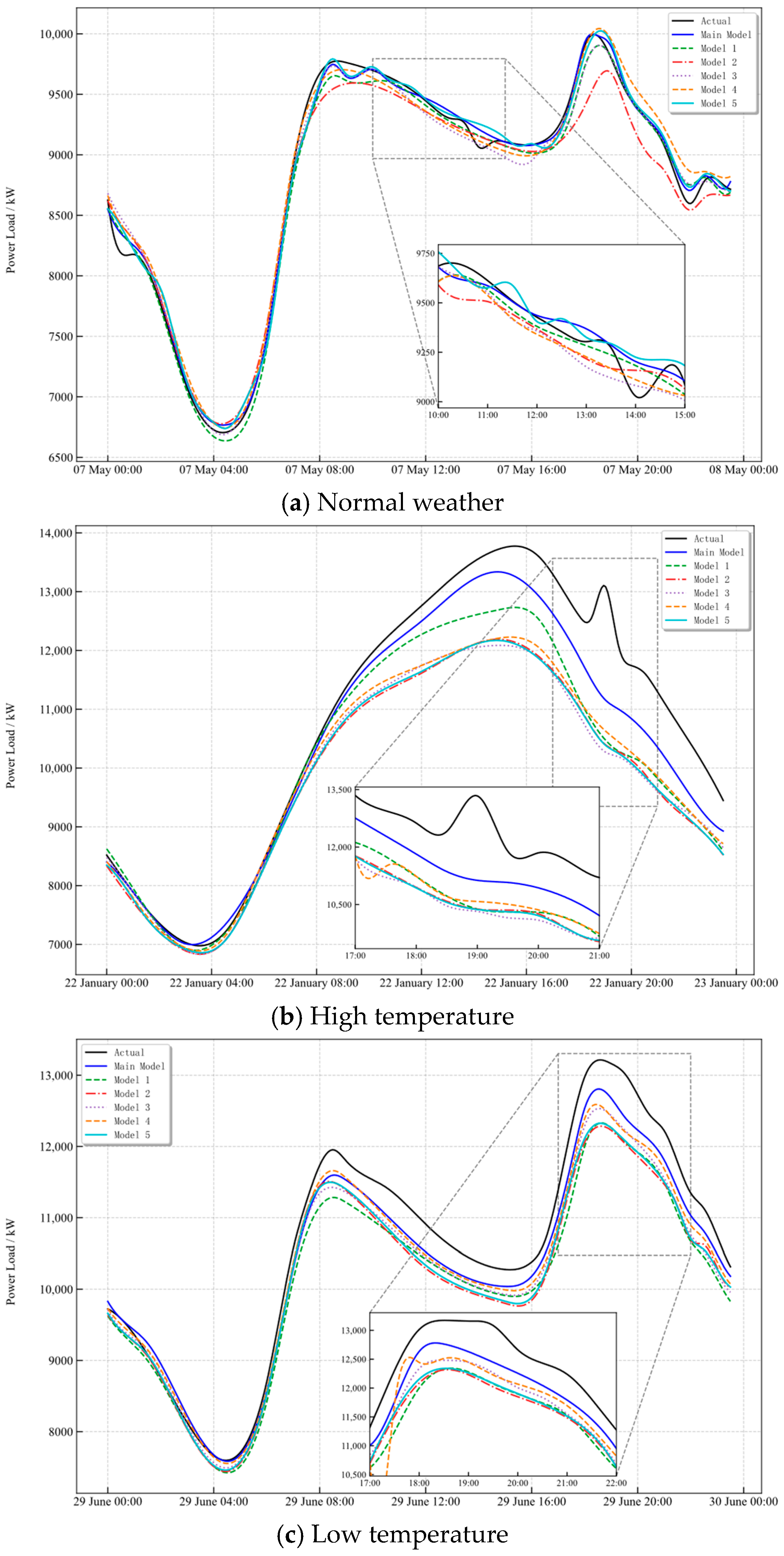
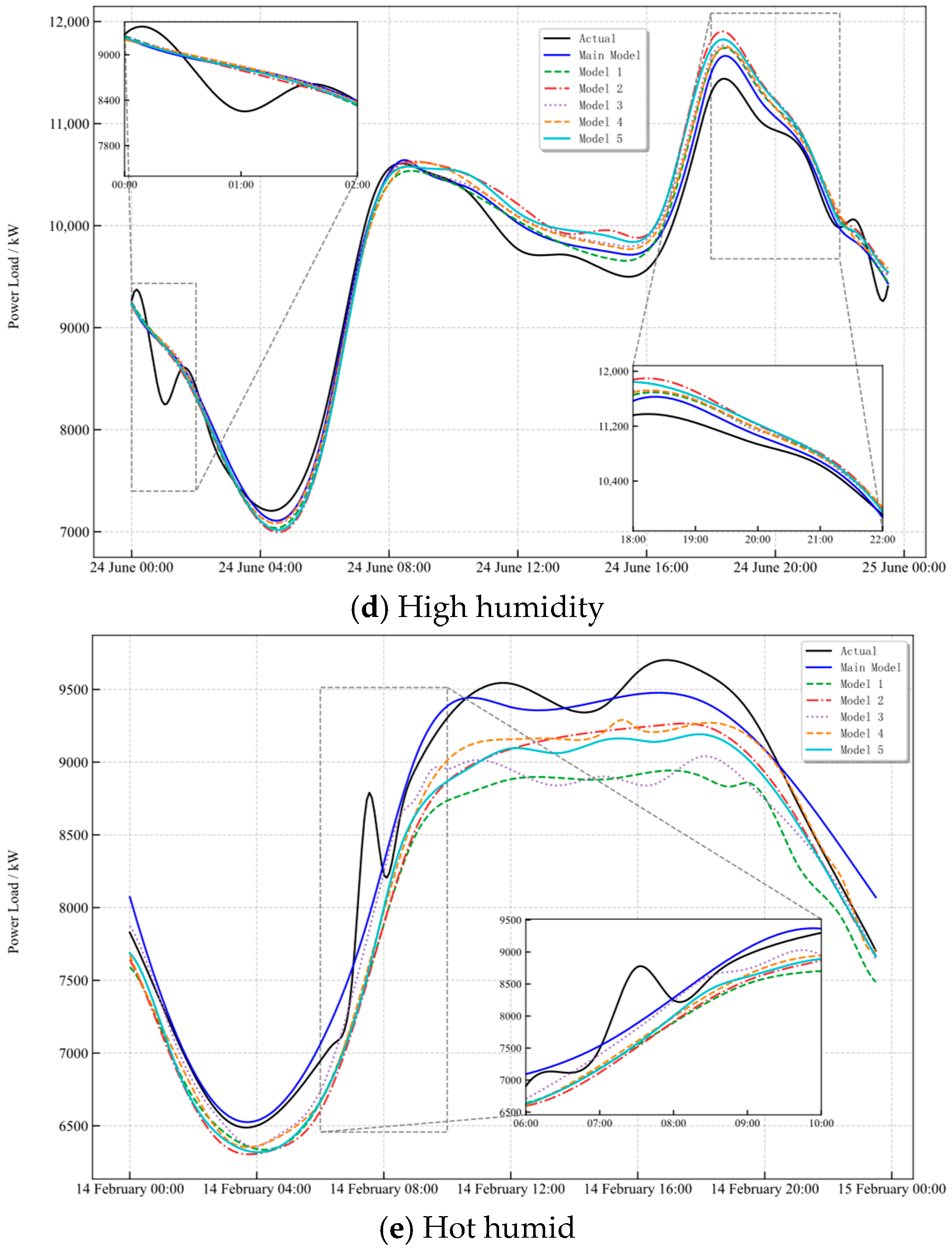
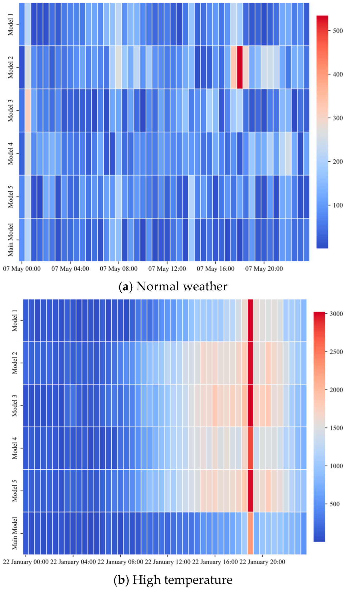
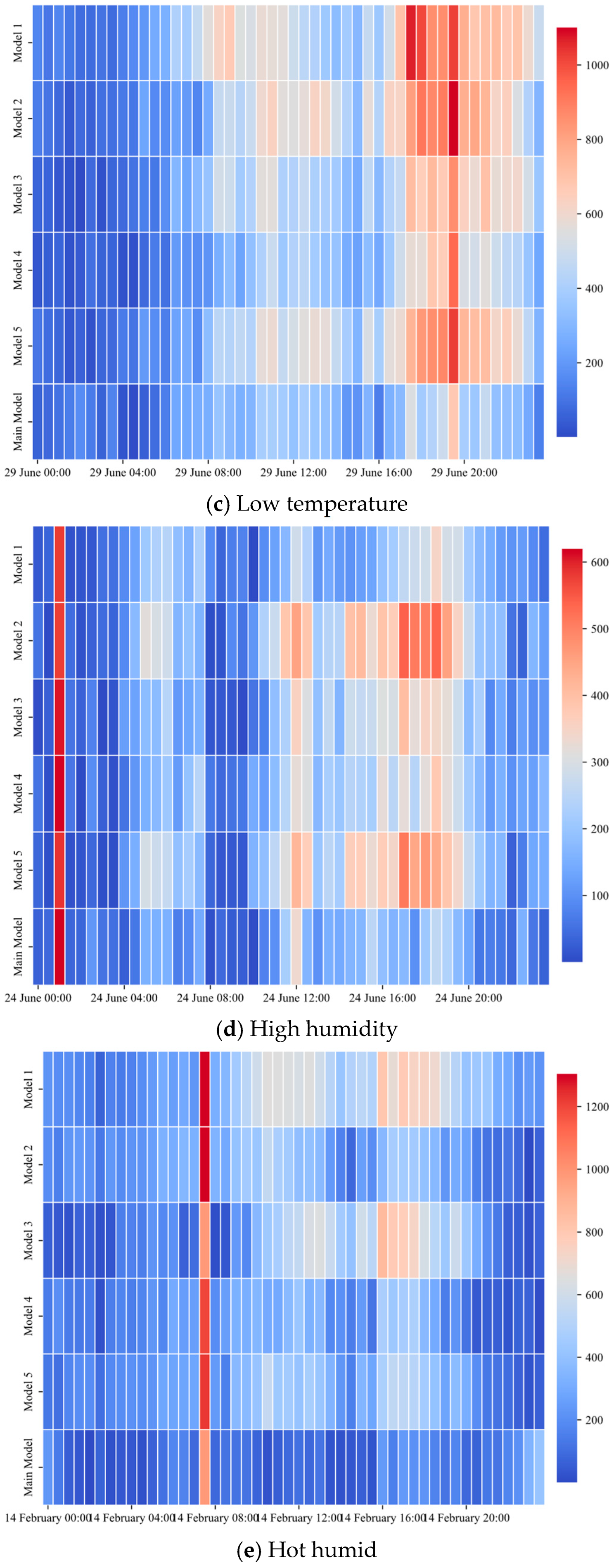
Across the five weather scenarios, as shown in Appendix A, Figure A5 and Figure A6, the proposed model attains higher fidelity around peaks and fast-varying segments. Error heat maps display low amplitudes and relatively uniform residual backgrounds, indicating effective suppression of time-specific bias.

Model 1. The dual-channel design is removed, and joint modeling of load and meteorology leads to mutual interference between their representations. In high-temperature and hot humid samples, contiguous high error bands emerge around peaks and adjacent rising segments. The waveforms show delayed peaks and reduced amplitudes, suggesting that the absence of channel separation weakens representation and localization of meteorological drivers.

Model 2. The self-attention enhancement in AE-BiGRU is removed. Without learnable time step weights, focus on key historical segments degrades. Continuous residual bands are more likely near peaks and through neighborhoods, with the morning and evening valley-to-peak phases of both normal weather and low-temperature samples being particularly sensitive.

Model 3. The feature fusion module is discarded and channel outputs are concatenated directly, which replaces dynamic matching with static stacking and removes cross-source alignment and fusion. In low-temperature and high humidity samples, alternating high error bands appear during evening rises and post peak declines, and the characterization of peak timing and amplitude becomes unstable.

Model 4. The learnable padding in CMCNN is removed and the kernel size is fixed to (3, 3). After the loss of multiscale and boundary adaptivity, segmental local error amplification is more likely around peaks and curve turning segments.

Model 5. The MIC gating unit is removed, which reduces the emphasis on key variables in the meteorological channel. Higher residuals tend to form around peak segments in high- and low-temperature samples.

Taken together, the synergy of dual-channel modeling, scenario-specific MIC weighting, feature fusion, and AE-BiGRU based sequence prediction effectively combines independent load and meteorological representations, scenario dependent variable emphasis, cross-source alignment, and temporal focus on key historical segments. Consequently, lower and more uniform residual distributions are observed across all five weather scenarios, consistent with the overall metric improvements in Appendix A, Table A4, which demonstrates stability and adaptability.

5. Conclusions

This study addressed the challenges posed by complex meteorological variations in multi scenario power load forecasting and proposed a short-term forecasting model based on DCFE. The main conclusions are as follows.

(1)

The dual-channel architecture enables independent modeling of load features and meteorological variables. In the meteorological channel, the MIC gating unit dynamically adjusts variable contributions by scenario. Cross-attention at a daily granularity level then fuses load and meteorological representations, which strengthens multi-source coordination and markedly improves adaptability and robustness under diverse weather conditions.

(2)

The CMCNN module, which combines multiscale kernels with a learnable boundary padding mechanism, enhances extraction of edge features and multiscale periodic information in the load sequence, thereby exhibiting greater stability under nonstationary meteorological influences.

(3)

The AE-BiGRU mitigates the attenuation of long sequence historical information through a self-attention enhancement mechanism and effectively highlights key temporal features. Learnable time step weights further focus on pivotal periods of load evolution and improve temporal modeling across weather scenarios.

(4)

Comparative visualizations of MIC gating weights and cross-attention matrices reveal the correspondence between variable contributions and day-level associations across scenarios. The inferred pathway from variable emphasis to cross-source alignment provides interpretability for the forecasts and enhances credibility and acceptability in engineering applications.