Abstract
The paper presents the findings of an analysis of a tank subjected to thermal effects caused by variations in air and liquid temperatures. The structural analysis focuses on the influence that thermal actions exert on the distribution of prestressing force. One of the important aspects addressed is the application of transient heat transfer analysis instead of the steady-state approach, allowing for a more accurate yet realistic representation of thermal effects within load combinations used to evaluate prestressing force. The study suggests that thermal actions should reflect the average annual temperatures of air and liquid separately, considering the transient thermal field. This hypothesis contradicts the standard approach. Numerical simulations using the finite element method were conducted in order to model transient heat transfer (CFD model) and the structural response of the tank (with axisymmetric shell model). The results indicated that temperature gradients across the tank wall may be linear or non-linear, varying with time and the amplitude of air temperature. Consequently, a modified formula for the reduced temperature gradient is proposed. The research emphasises the importance of incorporating transient thermal effects and the temperature-influenced distribution of prestressing force, which may have a significant impact on the safety of prestressed tanks.
1. Introduction
1.1. Literature Survey
Prestressing in cylindrical tanks is applied to effectively reduce tensile axial forces and control cracking. The prestressing force and its distribution depend on the structure’s dimensions and the required tightness class [1,2,3] or environmental exposure. However, this effectiveness decreases when bending moments arise, which may result from local boundary conditions or thermal effects [4]. Temperature is a particularly significant factor, as it influences not only wall thickness but also the properties of concrete, steel, and the prestressing forces. Thermally induced stress is stiffness-dependent, and its compensation is therefore challenging, potentially leading to cracking. This issue is critical in tanks storing liquids under varying thermal conditions, where significant temperature gradients can develop across the tank walls.
The position of the prestressing tendons presents another restriction. In the wall, they are located near the mid-surface or, at most, on the external surface, thus reducing the ability to adjust the force eccentricity. Thermal insulation would, of course, help mitigate thermal effects in the structure and reduce thermal stress formation. An alternative approach involves allowing limited-width cracking, which reduces stiffness but affects the tank’s watertightness. Therefore, accounting for thermal effects is essential, though complex, and is further complicated by the unclear provisions of design standards [1] and [5,6,7,8].
Numerous studies have investigated the thermal effects experienced by tanks and storage systems under varying environmental and operational conditions. Researchers have explored temperature-induced stresses, thermal gradients, cracking mechanisms, and the performance of different materials and reinforcement techniques. M. Priestley [9] focused on the behaviour of cylindrical tank walls under axisymmetric loads, emphasising the interaction between hoop tension and vertical bending. He introduced a frame analogy method to model the tank wall as a beam on an elastic foundation, allowing simulation of thickness variation and complex loading, including prestressing effects. H. Akita and Y. Ozaka [10] analysed temperature-induced stresses in cylindrical prestressed concrete water tanks, focusing on bending moments and tensile stresses caused by temperature gradients between the inner and outer surfaces of the tank wall. They conducted field measurements and finite element analyses of a 10,000 tonne water tank to determine a design temperature difference and assess thermal stresses and deformations. The study accounted for creep effects and seasonal and daily temperature variations and evaluated the accuracy of simplified and detailed computational models. E. Melerski [11] developed a numerical method based on elastic theory to evaluate the effects of temperature changes and shrinkage or swelling in circular concrete tanks used for storing liquids. The method assumed axial symmetry and a linear distribution of environmental effects (temperature or moisture) across the thickness of the tank walls and base. It was based on the concept of total potential energy and applied a force method-type approach, coupling separate analyses of wall and plate substructures. K. Reineck et al. [12] studied the development of cost-efficient, well-insulated hot water tanks designed for long-term thermal storage. Their research focused on replacing expensive stainless steel liners with high-performance concrete (HPC) and later with ultra-high-performance fibre reinforced concrete (UHPFRC) to improve structural efficiency and reduce costs. They analysed thermal stresses, crack control, insulation performance, and construction techniques.
J. Roetzer and D. Salvatore [13] carried out a numerical analysis of thermal effects on LNG tanks subjected to extreme temperatures of fire scenarios, including valve fires and fires from nearby sources. The study explained the calculation of heat radiation loads, the distribution of temperature in concrete structures over time, and the resulting reduction in stress and strength in materials. Based on a typical 150,000 m3 full-containment tank, the authors evaluated the non-linear temperature gradients caused by fire exposure and their impact on reinforced and prestressed concrete elements. A. Seruga and R. Szydłowski [14] introduced a method to prevent early-age thermal cracking in concrete tank walls by applying compressive stresses using unbonded tendons before the tensile stresses exceed the concrete’s tensile strength. Full-scale tests were carried out, along with materials laboratory investigations, and FEM modelling was used to analyse strain development. X. Cheng and X. Zhu [15] analysed the effects of thermal stress on the prestressed concrete outer walls of large LNG storage tanks in the other extreme conditions. Due to the extremely low temperature of liquefied natural gas, thermal stress can lead to cracking in the outer concrete wall. In their analysis, the authors evaluated the temperature distribution and optimised the arrangement of the prestressing tendons to reduce thermal deformation and stress. J. Rodriguez et al. [16] described the design, analysis, and construction of post-tensioned concrete digester tanks. The study focused on the use of circumferential and vertical post-tensioning systems to ensure crack-free and leak-tight tank walls under all load conditions, including seismic and thermal effects. X. Zhai et al. [17] studied the thermal stress behaviour of a 160,000 m3 liquefied natural gas concrete tank during the construction period using FEM. The analysis focused on predicting the temperature distribution and the resulting thermal stresses in the 800 mm thick outer concrete wall, aiming to identify potential cracking zones. The authors simulated the entire construction process, considering factors such as cement hydration, ambient temperature variations, concrete shrinkage, reinforcement ratio, and construction season. Y. Zhang [18] proposed an analysis method to study the thermal expansion characteristics of concrete in agricultural water conservation projects. Using FEM software, the study examined the effects of temperature, prestress, and mechanical properties on thermal expansion. The cooling method was used to model the prestress, and different modelling techniques were applied to assess the thermal expansion mechanism. Experimental validation confirmed the model’s ability to assess flexural bearing capacity and thermal expansion under varying erosion and material conditions. R. Wróblewski and J. Szołomicki [19] analysed a prestressed cylindrical tank considering thermal effects and variable water levels. They explored the influence of thermal loading on internal and prestressing forces in both serviceability and ultimate limit states. Eventually, K. Bouzelha et al. [20] conducted a semi-probabilistic assessment of partial safety factors for the top ring beam in circular reinforced concrete tanks. The analysis was performed using the First Order Reliability Method (FORM) and confirmed through Monte Carlo simulations.
Despite progress in understanding thermal effects in concrete water tanks, research in this domain remains limited. Therefore, the present study investigates thermal actions by the heat flow across the wall in a water tank and its influence on structural behaviour, offering new insights into the thermal performance of such structures and the implications for design in the serviceability limit state (SLS). The study therefore provides a foundation for the optimisation of prestressing force. This involves a numerical analysis of a prestressed concrete cylindrical water tank, considering thermal effects due to changes in air temperature and fluctuations in liquid level and temperature. The aim is to assess how these thermal actions affect the required prestressing reinforcement. FEM simulations were performed using a computational fluid dynamics (CFD) model [21] and structural analysis software [22]. The findings of this study underscore the significance of transient heat transfer analysis and the necessity to modify the prevailing design approach for temperature distribution. The current approach, as outlined in standard [8], is found to be unrealistic and results in ineffective prestressing of tanks. Therefore, a novel approach to modelling temperature effects within the quasi-permanent load combination is proposed and examined. The outcomes of this approach are evaluated using a real-world design of a prestressed concrete tank. The relevance of this investigation lies in its direct applicability to both the structural design of new tanks and the assessment of existing infrastructure.
1.2. Problems of Modelling Thermal Actions in Tanks
Thermal stress during the operation and construction of a concrete tank can result from several natural and technological phenomena: heat released during cement hydration, temperature changes in the structure caused by air and liquid temperature, as well as sunlight exposure. Their precise consideration is possible a posteriori, when measured data is available and operating conditions are known. In contrast, at the design stage, models are used to predict these phenomena. However, there are some exceptions: standard [7] (B.2.3) allows the omission of stresses caused by thermal actions in the ultimate limit state when there is no risk of fatigue or low-cycle plastic failure; a similar approach is applied in [5] (2.3.1.2), requiring sufficient ductility, and in [6] (4.2.1.3), requiring sufficient deformation capacity.
When thermal actions are considered at the serviceability limit states, discrepancies arise between buildings, bridges, and tanks, as well as between tanks and silos [23]. These discrepancies result from the temperature of the stored medium, the ambient temperature, and their variations. The quasi-permanent value of the effect of a variable action Qk, used for the verification of long-term effects, can be determined as the average over a period of time [24] and is represented in [25] as Ψ2Qk. Thus, the characteristic values of Qk (with a typical annual exceedance probability of 0.02) can be reduced to a mean or median value. In limit state design [25], this issue is reduced to the value of factors for temperature actions Ψ2. As outlined in [7,25], factor Ψ2 remains a single constant value, disregarding seasonal temperature variations. Therefore, as demonstrated in Table A.5 of the standard pertaining to actions in tanks [7], the factor for the quasi-permanent value of temperature is Ψ2 = 0. However, it is difficult to justify in a tank with warm or hot liquid and without thermal insulation [23], since the wall of such a tank is continuously subjected to internal thermal action. In bridge design, where structures are constantly exposed to temperature variations, Ψ2 = 0.5 is adopted, as presented in Tables A2.1, A2.2, and A2.3 of [25], which may be an overestimate for tanks. Furthermore, adopting the same Ψ2 factor as for medium pressure load seems unreasonable, as air temperature constantly fluctuates from the initial temperature T0, even if the liquid temperature remains constant. It may also be important to note how quickly the stored liquid can cool down or heat up. Therefore, considering Ψ2Qk as the temperature-averaged effect [24], the air temperature remains constant because in A.1(3) of [8] the initial temperature T0 is the same as the yearly average air temperature: T0 = Tout,m, even though the air temperature fluctuates between Tmax − T0 and Tmin − T0. In the same way, the temperature of the liquid represented by Ψ2Qk should be the yearly average temperature of the liquid Tin,m. Hence, the temperatures Tout,m and Tin,m on both surfaces can be considered as a representation of the quasi-permanent action Ψ2,outQk,out = Tout,m and Ψ2,inQk,in = Tin,m. In this context, although it may be difficult to determine a common value of Ψ2 (Ψ2,out = Ψ2,in) for both air and liquid, the steady-state temperature distribution can still be applied. However, this approach does not account for the inevitable variation in air temperature over time, which should be estimated based on the time required for the transient temperature distribution to reach a steady state. Therefore, the standard temperature action model [8] should be modified for tank applications.
Typically, the distribution of temperature across the tank wall is represented as a result of the steady-state temperature field. However, some measurement data [26] show a non-linear cross-section temperature distribution, confirming the existence of a transient temperature field. The recorded temperatures on the external surface of a 400 mm thick wall were significantly different from the air temperature, which reduced the temperature gradient by about 40%. This phenomenon occurs due to heat transfer from the higher-temperature liquid to the tank’s outer surface, resulting in a surface temperature that exceeds the surrounding ambient air temperature. However, in a concrete tank design, the ambient air temperature is applied to the external surface of the tank [8]. It is posited that, in view of the analysis results, a new method should be adopted in lieu of the existing standard approach for the purpose of enhancing the effectiveness of prestress considered in any tank design. However, the potential impact of this approach is constrained by additional restrictions imposed in the design standard [6].
The phenomenon of transient heat transfer has already been considered earlier in [27] and [28] and was also applied in the 1989 version of [29], where the adjusted temperature gradient ∆ϑ in the walls of the silos was obtained from the following relation:
where h—wall thickness in [m], ∆t—temperature difference on the surfaces of the structure (i.e., steady-state temperature field). Thus, the resulting bending moment was obtained in the following form:
where —coefficient of thermal expansion, —modulus of elasticity and ν—Poisson’s ratio of concrete.
The use of Equation (2) can be applied to any panel, wall, slab, or shell, disregarding a spatial structural system, and the values obtained using Equation (2) are likely to underestimate bending moments [30]. The simplification of thermal stress distribution to a linear form may lead to inaccuracies when a time-dependent temperature distribution is present. In such cases, the actual temperature profile across the cross-section is often non-linear, resulting in a more complex stress state. Unlike a linear distribution, a non-linear temperature field can generate not only bending moments but also axial forces due to asymmetric or uneven expansion. Therefore, when evaluating thermal effects under transient conditions, both bending and axial effects should be taken into account to avoid underestimating the structural response. It should be mentioned that cracking makes the determination of stiffness complicated. Its reduction is allowed by [5], but no method or degree of such reduction is provided, which is crucial from the perspective of the bending moment values. In the case of uncracked walls, the potential uncertainty may concern creep deformations. A less significant issue is the discontinuous temperature distribution in the ground surrounding the tank assumed in [8]. At the ground surface and at a depth of 1 metre, the temperature is assumed discontinuous, and unrealistic internal force distributions are obtained.
Although experimental research conducted by P. M. Piotrkowski and T. Godycki-Ćwirko [26] has demonstrated that the temperature distribution within the concrete tank walls is distinct from that of a steady state, analyses of the structural response to this phenomenon have not been conducted. Therefore, the paper demonstrates the irrelevance of using steady-state heat transfer in tank design, proposing instead a novel adjusted temperature gradient formula. It also suggests a novel approach for representing thermal loads in quasi-permanent load combinations. Furthermore, the text explores a pivotal subject concerning the structural safety and serviceability of prestressed concrete water tanks related to temperature actions. It is claimed that the temperature actions may result in over-prestressing of the tank in SLS prior to ULS, a phenomenon that has the potential to compromise the structural safety.
2. Materials and Methods
2.1. Thermal Field Analysis
The analysis utilised a cylindrical prestressed water tank, as presented in Figure 1. Due to the vertical axis-aligned rotational symmetry of both the tank and the actions, adopting a reduced model was found suitable for examining thermal effects. Therefore, a 2-dimensional CFD model based on FEM [21] was utilised to simulate thermal behaviour (Figure 1). Furthermore, the analysed segment of the prestressed concrete tank wall proved sufficient for capturing transient heat transfer phenomena in the tank. The parameters presented in Table 1, as outlined for the concrete in [31], were utilised in the initial analysis.
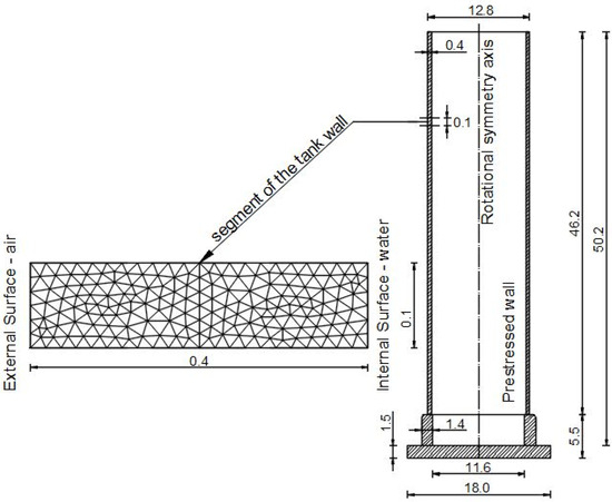
Figure 1.
Vertical cross-section of the cylindrical prestressed water tank (dimensions in m) and a segment of the tank wall (with FE mesh) used as the 2D model in CFD simulations.

Table 1.
Material properties.
As highlighted in Table 2, not every parameter listed in Table 1 shows data variability (in an approximate temperature range of −20–+30 °C), suggesting levels of uncertainty ranging from negligible to extremely high. Factors affecting the thermal properties of concrete include moisture content, temperature, composition (mostly aggregate properties), and porosity. Convection coefficients are significantly influenced by the type of convection and the parameters associated with forced (assisted) convection.
Table 2.
Uncertainty of material properties.
The water convection coefficient was considered to be relatively high since the tank functions as an energy storage unit. Because water is not kept in the tank for extended durations and instead undergoes regular cycles of filling and emptying, a free convection condition was dismissed, and the convection coefficient was adjusted to reflect a value suitable for assisted convection. The air convection coefficient does not consider surface roughness or wind. Nevertheless, on nights when air temperatures drop to around −20 °C, the wind generally does not occur in the region.
Within the software, convection is simplified by using constant coefficients that are directly input, as the temperature distribution needed to be assessed only inside the wall. Thus, thermal conductivity, specific heat, and density of water and air remained unused (Table 1). Consequently, the water and air were substituted by convection boundary conditions applied to the wall surfaces, in conjunction with the temperatures of both the water and air. The air temperature varied, while the water temperature remained unchanged.
The parameter ranges presented in Table 2 were applied for a sensitivity analysis, detailed in Appendix A. An assessment of transient heat transfer, employing sinusoidal air temperature fluctuations (period 24 h = 86,400 s, initial temperature −15 °C, amplitude 5 °C), examined how parameters affect the temperature on the wall’s external surface (Figure 1). Findings indicated that concrete’s thermal conductivity and air convection coefficients significantly affect the resulting temperature, while other parameters had minimal effects. This suggests that the findings could display variability since key parameters were assumed rather than measured, as shown, for example, in Figure 2. These results highlight the necessity of examining concrete conductivity and integrating environmental factors into the air convection coefficient model.
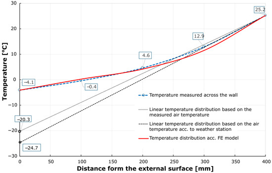
Figure 2.
Temperature distribution recorded in winter 2010 across the tank’s wall at the time of the lowest air temperature recorded, 24 January 2010 at 8:30 (based on [26]), along with the results from the FE transient heat transfer model (fitting the FE model to the temperature measured across the wall, RMSE = 0.729).
To proceed with the sensitivity analysis, a mesh size of 0.018 m and a 36 s time step were selected, adhering to the same criterion. These selections ensured precise results, with differences less than 0.0004% (Table A6 and Table A7 in Appendix A) compared to denser configurations. The software does not disclose specific numerical criteria for convergence, such as total or incremental residuals. Instead, it automatically modifies iteration limits and error tolerances. The user can define solution precision and modify the mesh to assess convergence, which was implemented.
Subsequently, the FE model was validated based on the experimental data provided in [26] (Figure 2 and Figure 3). As the temporal variation in the temperature of the wall’s external surface was also obtained from the FE model (Figure 3), this is presented to demonstrate the difference between transient and steady-state field temperatures. In the latter case, the external surface temperature is almost identical to the air temperature.
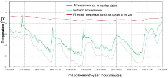
Figure 3.
Air temperature recorded in a period of 5 days in winter 2010 (reproduced with the permission of the author [26]), along with the results from the FE transient heat transfer model.
Afterwards, the model was utilised to simulate the temporal temperature distribution in the wall under various air temperature actions, examining the influence of temperature amplitude. The constant water temperature of 25.2 °C and alternating air temperature over a period of 5 days (432,000 s) were assumed. The applied cases of external air temperature followed sinusoidal functions with a period of 24 h (86,400 s), as presented in Table 3 and Figure 4. As the outputs of the analysis were governed by temperature variations and their rate of change, the sinusoidal function was used to represent the model input temperature continuously. This idealised temperature model allows for capturing the essential characteristics of daily temperature fluctuations in the form of a continuous function while ensuring computational stability and repeatability. It also facilitates comparative analysis of thermal responses under cyclic loading and helps identify general trends in transient heat transfer through the tank wall. Furthermore, the assumed external temperature distribution may represent an extreme situation, such as a period of very cold weather lasting a few days in winter. A real example of this is presented in Figure 3.
Table 3.
External air temperature distributions according to a sinus function.
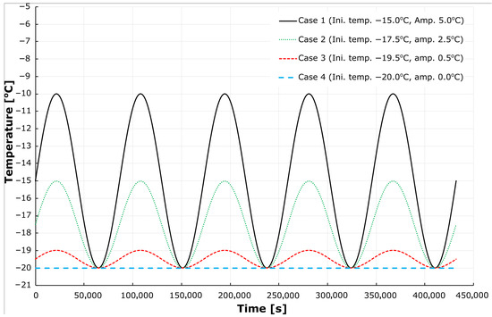
Figure 4.
Cases of the air temperature distribution in time.
In all cases, a minimum temperature of −20 °C was adopted, with the external surface temperature presented in Figure 2 being referenced, albeit with different temporal scenarios. Additionally, further analyses were carried out with various wall thicknesses (ranging from 300 mm to 600 mm) to assess their influence on the temperature at the outer surface of the wall.
2.2. Structural Analysis
The structural FE simulations of the tank presented in Figure 1 were conducted utilising an axisymmetric shell model (Figure 5a), given that the vertical axis-aligned rotational symmetry of the tank, loads, and prestressing permits this approach [32,33]. As the analysed model is more complicated than that presented, for example, in [4], double verification of the credibility of outcomes from this model was processed; that is, based on the following:

Figure 5.
Models of the tank: (a) axisymmetric shell model—whole tank (left) and a bottom part (right); (b) 3D axisymmetric solid model—whole tank (left) and a bottom part (right). In both models, the “0” of the x-axis is situated at the same position, i.e., at the joint of the socle and the top wall that was prestressed.
- -
- A thermally loaded tank example given in [4];
- -
- A 3D axisymmetric solid model (Figure 5b), as it represents a more rigorous analysis approach than an axisymmetric shell model.
Differences in results between shell and solid models in estimating internal forces are presented in Table 4. They show that in structural analysis, care must be taken in the areas of the wall at the water level.
As cracking was not permitted in the tank, all simulations were carried out under the assumptions of small displacements and strains, as well as a linear-elastic material model. The tank foundation was modelled using spring supports, assuming a well-prepared subgrade with a spring stiffness of k = 15,000 kN/m3.
In accordance with the stipulated design parameters, concrete of class C30/37 was employed, incorporating standard steel reinforcement of type B500B with a yield strength of fyk = 500 MPa and prestressing steel of type St1660/1860 with strands consisting of 4 tendons Ø15.7 mm (150 mm2) placed in internal ducts. A low-friction, bondless system was applied to the top part of the tank, where a wall thickness of 400 mm was designed (Figure 1 and Figure 5). In the calculations for the spacing of the prestressing tendons, the losses of prestressing force were taken into account under the assumption of alternating anchoring of adjacent tendons every 180°, resulting in an almost uniform distribution of prestress around the circumference. Time-dependent losses were subjected to variation in accordance with the results of actions in quasi-permanent load combinations.
It was assumed that in the serviceability limit state (SLS), the prestressing force would counteract the circumferential tensile force, while the ordinary circumferential reinforcement would resist the bending moments. In the ultimate limit state (ULS), the required prestressing force was intended to balance the stresses on the wall surfaces, making the presence of ordinary reinforcement less significant in this case.
It was also assumed that the walls of the tank would remain uncracked under the frequent load combination within the SLS [25] and that no decompression would happen under the quasi-permanent load combination [25]. It is evident that these assumptions override the requirements given in Section 7.3.1(6) and Table 7.1N of [5] and in Table 9.2 of [6]. This is due to the fact that Tightness Class 3 (Table 7.105 in [1]) and Tightness Class TC3 (Table H.1 in [6]) were required not to permit any leakage. The assumption disallowing cracking does not guarantee tightness and the absence of cracks throughout the whole service life. This is due to the fact that the real actions to which the tank may be subjected may exceed the loads imposed by frequent load combinations assumed in the design, given that the loads have a probability of being exceeded. The appearance of cracks in any tank may also be influenced by interacting phenomena in concrete, including tensile softening, tension stiffening, creep under thermal gradients, and moisture transport with thermal dilation coupling. The tank that was the subject of the analysis was designed to incorporate ordinary reinforcement, thereby enabling the tension stiffening effect to be achieved. This effect allows for larger deformations before crack appearance than would be the case in a ‘pure’ concrete. This phenomenon, associated with tensile softening, exerts an influence on the crack width and spacing [36,37]. It is evident that an augmentation in the reinforcement ratio engenders a reduction in both variables. Nonetheless, the aforementioned increase has the potential to result in premature cracking, a consequence of the shrinkage. Crack propagation contributes to stiffness loss, thereby influencing the structural performance [36,38] by reducing the effects of actions imposed by restraints, such as temperature.
When concrete in the tank wall is exposed to temperature variations, it undergoes uneven expansion or contraction that leads to tensile stresses in the cooler areas, potentially causing cracks [39]. Concrete creep initiates soon after the stress emerges, affecting stress relaxation, its redistribution to reinforcements, and deformation over time under non-uniform thermal conditions. These partially irreversible deformations increase with stress levels and can assist in alleviating thermal stresses by relaxing some of the induced tensile stress and reducing the immediate likelihood of cracking. This is particularly significant at high temperatures and in young concrete [39,40]. In the analysed case, the effects of temperature-induced creep might be less significant than those generated by prestressing, given the presence of seasonal temperature gradients resulting from variations in water and ambient conditions. In addition, the tank will undergo frequent cycles of filling and emptying, which further diminishes the gradients. However, exposure to solar radiation can possibly result in cracking in the southwest area and can also cause thermal creep in the tank [40]. Cracking can be linked with an increase in pore pressure and water migration in concrete due to heating, which can weaken the cement matrix.
Thermal expansion alongside moisture transport influences the volume stability and mechanical properties of concrete, such as thermal expansion, elasticity modulus, and strength [41], leading to internal stress and increasing crack susceptibility [42,43]. This coupled hygro-thermal-mechanical effect can be substantial in the tank, given its exposure to moisture and temperature fluctuations that generate cyclic stress, speed up fatigue, and contribute to material degradation, underscoring the importance of these phenomena for the structure’s durability [42].
For temperature actions (excluding exposure to sunlight in quasi-permanent load combinations), the following combination coefficients were used: Ψ0 = 0.6, Ψ2 = 0.0–0.70. The values of Ψ0 = 0.6 and Ψ2 = 0.0 are listed in Table A.5 of [7]. However, as outlined in Section 1.2 of this paper, Ψ2 was gradually increased in order to examine its effects. In the SLS, the shrinkage action was neglected because the difference in shrinkage strains in the socle and in the wall after approximately 15 years generates compressive forces in the prestressed wall (Figure 6). Moreover, even temporary filling with water reduces shrinkage. However, in the ULS, the shrinkage action was considered after 616 days, when the maximum difference in shrinkage strains occurs (Figure 6).
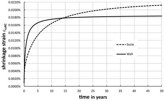
Figure 6.
Concrete shrinkage strains reduced by reinforcement εcsRC.
The loads were determined based on standards [7,8,44] with consideration given to the variation in water levels and water temperatures in summer and winter as outlined in Appendix B. Load combinations were applied in accordance with tables A.1 and A.5 of [7] with partial safety factors in ULS considering favourable and unfavourable effects as stated in table A1.2(B) of [25] for (Equation 6.10). And the required prestressing force should always meet all the following conditions [5]:
- (1)
- In the ULS (fundamental combinations)—γP·Pm,t ≥ NφEd.
- (2)
- In the SLS (frequent combinations)—rinf·Pm,t ≥ Nφcr, i.e., cracking force.
- (3)
- In the SLS (quasi-permanent combinations)—rinf·Pm,t ≥ Nφdec, i.e., decompression force.
where
γP—partial safety factor for prestressing force according to Section 5.10.8 of [5]; Pm,t—mean prestressing force at time t; NφEd—the circumferential axial force due to load effects in ULS; Nφcr—the circumferential axial force that causes cracking in the cross-section; rinf—factor considering variation in prestressing according to Section 5.10.9 of [5]; Nφdec—the circumferential axial force that causes decompression in the cross-section.
3. Results
3.1. Thermal Field Analysis
The temperature amplitude on the external surface of the wall was reduced by 40% in cases 1–3 (Figure 7), compared to the air temperature (Figure 4). Furthermore, the average temperature on the external surface of the wall depended on the amplitude of the air temperature and decreased from −9 °C in case 1 (amplitude 5 °C) to −13 °C in case 3 (amplitude 0.5 °C). As illustrated in Case 4, where the amplitude was set to 0 °C, this particular case yielded an asymptotic result indicative of the influence of the amplitude, as well as the minimum temperature, on the surface of the wall (approximately −13.5 °C in Figure 7).
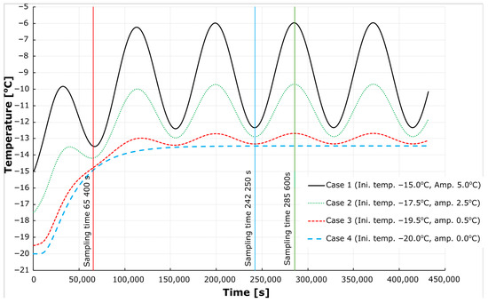
Figure 7.
Temperature distribution over time on the external surface of the wall based on FE model.
The function of temperature distribution (linear or non-linear) across the wall thickness depended on the time of sampling and the air temperature amplitude (Figure 7, Figure 8 and Figure 9). With a small amplitude (cases 3 and 4) and sampling at the minimum air temperature (Figure 8), the distribution tended to be non-linear and was linearised when the air temperature reached its maximum (Figure 9). The opposite effect was observed when analysing the large-amplitude case 1.
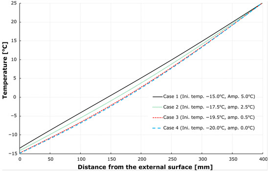
Figure 8.
Temperature distribution across the wall thickness at the minimum air temperature (sampling time 65,400 s).
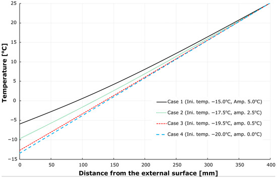
Figure 9.
Temperature distribution across the wall thickness at the maximum air temperature (sampling time 285,600 s).
The influence of the wall thickness on the temperature on the external surface (thus the temperature gradient) was more pronounced for a smaller wall thickness (Figure 10), which can be attributed to the increased speed of the heat transfer (or lower thermal resistance) as the thickness decreases.
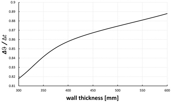
Figure 10.
Relative adjusted temperature gradient ∆ϑ across the wall as a function of the wall thickness.
3.2. Structural Analysis
The three most important findings of the structural analysis concerning the prestressing force distribution were as follows:
- With the quasi-permanent value factor of the temperature action Ψ2 ≈ 0.25–0.35, the required prestressing force in the SLS was similar when based on the cracking criterion (frequent load combinations with summer and winter temperatures considered) and decompression criterion (quasi-permanent load combinations with summer and winter temperatures considered) (Figure 11).
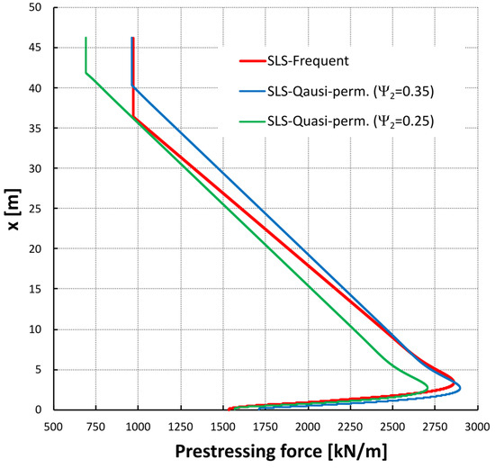 Figure 11. Required prestressing force in the SLS as a result of summer and winter temperatures.
 - With an increase in the quasi-permanent value factor to Ψ2 ≈ 0.37, the prestressing force in SLS was based exclusively on the decompression criterion. However, it should be noted that this was only applicable to the summer temperature over a short distance (2 m for the tank filled to ¾ and 4 m for a full tank). The prestressing force over the remainder of the wall was governed by the prevailing winter temperatures. The prestressing force was governed by the criteria for decompression and cracking when Ψ2 < 0.37.
- Depending on the value of Ψ2, in the upper part of the tank (25–30 m in Figure 12), the prestressing force required by the SLS was greater than that required by the ULS, which may lead to over-prestressing; that is, cracks would not occur before failure of the prestressing steel, potentially resulting in sudden collapse. For the value of Ψ2 ≈ 0.70, over-prestressing would occur along the entire height of the tank wall (Figure 12).
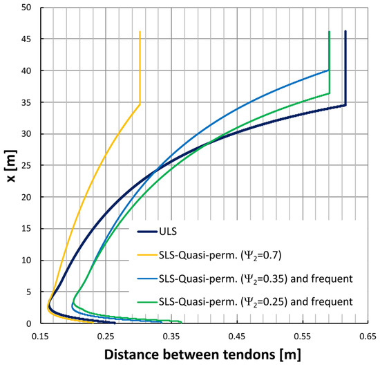 Figure 12. Spacing of prestressing tendons as a result of both summer and winter temperatures, and in SLS additionally as a result of the quasi-permanent and the frequent load combinations.
4. Discussion
The steady-state temperature distribution usually assumed in the design overestimates temperature gradients, as presented in [26] and obtained from models based on transient heat transfer. The temperature gradient across the uninsulated concrete wall is invariably diminished, as the outer surface does not attain the same temperature as the ambient air. This reduction was found to be stable and asymptotic in the conducted simulations. Therefore, it is believed that these asymptotic values (case 4 in Figure 7, Figure 8 and Figure 9) can be considered as a safe estimation for design purposes.
As demonstrated in the experimental results [26], on the day with the lowest air temperature (Figure 2), the values of Δt, Δϑ and Δϑ/Δt were found to be 25.2 + 20.3 = 45.5 °C, 25.2 + 4.1 = 29.3 °C, and 0.64, respectively. The result obtained from Equation (1) for the 400 mm thick wall is Δϑ/Δt = 0.53, overestimating both the experimental and case 4 (Table 5) reductions. Consequently, this equation cannot be utilised in tanks.
Table 5.
Temperatures of the air, the liquid, and the tank’s wall (sampling time 242,250 s).
The incongruity between case 4 and the experimental results can be attributed to the fact that the temporal air temperature distribution (Figure 3) was considerably more intricate, which may render it unfeasible to draw comparisons with case 4. However, a comparison of the air temperature in this case with that in case 1 reveals a degree of similarity, attributable to the presence of a cyclic behaviour and the amplitude value. This similarity can be evidenced by the fact that the amplitude in the experiment varied from approximately 3 to 7 °C (Figure 3) and was assumed to be 5 °C in case 1.
The FEM results presented in Figure 10 and Figure 13 were obtained from case 4 with the difference between liquid and air temperature Δt = 45.2 °C (Table 5). In the case of the 400 mm-thick wall under scrutiny, the temperature on its outer surface exhibited an increase in comparison to the ambient air temperature (Figure 7 and Table 5). This phenomenon led to a reduction in the ratio Δϑ/Δt (relative adjusted gradient) for cases 1 to 3 with non-zero amplitude, as compared to case 4 with zero amplitude (Table 5). It was demonstrated that the ratio Δϑ/Δt is contingent on the amplitude of air temperature and attains its maximum value for zero amplitude. This is equivalent to case 4 being the asymptotic case. It must be acknowledged that this particular case lacks realism, yet it remains a secure option. Nevertheless, it is possible to identify and model a number of more realistic scenarios on the basis of long-term meteorological data.
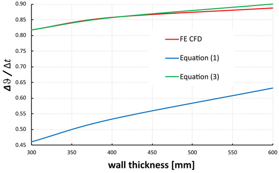
Figure 13.
Relative adjusted temperature gradient as a function of wall thickness (fitting Equation (3) to FEM CFD RMSE = 0.0071).
Moreover, the gradient reduction depends on the wall thickness, and it was found that modification of Equation (1) to Equation (3) (with utilisation of the Newton–Rapson procedure to obtain a constant 0.0665 m) well fits (RMSE = 0.0071) the transient analysis results (Figure 13):
The reduction obtained from Equation (3) is significantly lower than that in Equation (1). However, this finding aligns with Buczkowski’s [30] indication regarding the necessity to augment bending moments, yet it is not attributable to transient heat transfer but rather to the spatial behaviour of the structures.
Based on the adjusted gradient given in Equation (3), an alternative approach for representing thermal loads in the quasi-permanent load combination was developed to assess Ψ2. A medium value of the temperature gradient was used, which, in this approach, makes the value of Ψ2 dependent on the thickness of the wall. And in the case of the tank [26] with a liquid temperature of 25.2 °C:
- −
- The initial temperature was the same as the annual average air temperature T0 = Te,m = 8.0 °C according to A.1(3) of the national annex of [8].
- −
- Average water temperature Ti,m = 25.2 °C.
- −
- The resulting gradient = Ti,m − Te,m = 17.2 °C and the adjusted gradient value = 14.75 °C.
- −
- The characteristic winter temperatures in the region Tmin = −26.0 °C (according to A.1(1) of the national annex of [8]) resulted in the gradient = Ti,m − Tmin = 51.2 °C and the adjusted gradient value = 43.90 °C.
- −
- Considering Ψ2 as a ratio of an average value to the characteristic one Ψ2 (h = 400 mm) = = 0.34 ≈ 0.35.
It is important to emphasise that this approach deviates from the conventional method [25] in that Ψ2 is not uniform for summer and winter; consequently, Ψ2Qk should be sought (after which Ψ2 can be calculated). It can thus be concluded that Ψ2Qk differs for Tmin in comparison to Tmax, as demonstrated in the following example of the analysed prestressed tank:
- −
- The initial temperature was assumed to be equal to the annual average air temperature: T0 = Te,m = 10.0 °C according to A.1(3) of the other national annex of [8].
- −
- The average water temperature: in winter Ti,m = 4.0 °C and in summer Ti,m = 10 °C.
- −
- The resulting winter gradient: = Ti,m − Te,m = −6.0 °C and the adjusted gradient value: = −5.14 °C.
- −
- In summer: = Ti,m − Te,m = 0 °C.
- −
- The characteristic winter temperature in the region is Tmin = −27.0 °C, which resulted in the gradient of = Ti,m − Tmin = 31.0 °C and the adjusted gradient value of = 25.58 °C.
- −
- Winter: Ψ2 (h = 400 mm) = = −0.19 ≈ −0.20.
- −
- The characteristic summer temperatures in the region was Tmax = 37.0 °C (according to A.1(1) of the national annex of [8]), resulting in the gradient of = Ti,m − Tmax = −30.0 °C and an the adjusted gradient value = −25.72 °C.
- −
- Summer: Ψ2 (h = 400 mm) = = 0 because = 0.
However, different values of Ψ2 can be obtained when the average annual liquid temperature is taken into account, Ti,m = 7.0 °C, resulting in low values of Ψ2: for winter, Ψ2 = −0.10 and for summer, 0.05. Nevertheless, all the obtained Ψ2 values are too small to be used for determining the prestressing force. As shown in Figure 11 and Figure 12, Ψ2 > 0.25–0.35 was considered a significant value; however, in other tanks, the governing Ψ2 values may differ. An additional issue concerns the interpretation and applicability of Ψ2 < 0.
As a consequence of the results presented in Section 3.2, the increase of Ψ2 may significantly reduce overall structural safety by over-prestressing. Therefore, the use of high ductility reinforcement (along with prestressing one), as a tying system protecting the structure against progressive collapse, can be used. This combination of reinforcement can be necessary, as the deformation of prestressing steel is approximately 2 to 3 times smaller than high ductility steel. The area of the auxiliary reinforcements may be determined by the difference in prestressing force between the SLS and the ULS. Alternatively, partial prestressing can be used to permit cracking, utilising smaller values of Ψ2.
The results presented herein consider the effects of shrinkage in ULS directly by introducing a load case to assess tensile circumferential forces in the shell after 616 days. This is based on the assumption that the tank will not be filled during this time. However, it should be noted that in a tank filled with water, drying shrinkage does not develop, and instead, swelling may occur. This is only partly applicable to the tank under analysis, given that its design involves periodic filling and emptying. Furthermore, it can be concluded that the shrinkage effects are reduced by the interaction of shrinkage and creep. This is due to the fact that creep serves to diminish shrinkage stress after prestressing. This interaction is ongoing and is in accordance with the cycles of water evaporation from concrete. It is hypothesised that both shrinkage and creep do not impact the results obtained. In contrast to the effect of shrinkage, the effect of swelling may be negligible due to the generally high waterproofing of the concrete used in the tanks.
Nevertheless, it is important to note that there is a possibility of the occurrence of deleterious effects, such as a moisture gradient, which may have an impact on the results. This is due to the fact that an increase in water content within the internal parts of the tank wall serves to reduce shrinkage and increase heat transfer. This may result in the manifestation of an imbalance in stress distribution across the wall, thereby giving rise to tensile stress in the external regions. In this particular context, an external position of the tendons in the cross-section may have a role to play in the reduction in this tensile stress. In the analysed case, the estimated long-term increase in compression stress due to the change in position of the tendon to the external surface was found to be equal to σce = Pm,t·(h/2 + dp/2)/(h2/6) ≈ 603·(0.4/2 + 0.0157/2)/(0.42/6) ≈ 2439 kN/m2 ≈ 2.4 MPa. This is not a negligible value, given the values of the concrete tensile strength fctm = 2.9 MPa.
5. Design Recommendations
The omission of stresses caused by thermal actions at the ultimate limit state, under certain restrictions, is a rational solution, as stiffness is significantly reduced at this stage, leading to a reduction in thermally induced stress. Therefore, it is recommended that the provision in [6] (Section 4.2.1.3 point (2)) is used, as the most relevant to the design of the water tanks. This section requires “sufficient deformation capacity”, which can be achieved by reinforcement ductility.
With regard to the stress calculation, notes 3 and 4 can be used to supplement Section 4.2.1.3 point (1) of [6]:
NOTE 3 The adjusted temperature differentials in uninsulated concrete water tank walls can be assumed in linear elastic stress analysis:
where
is a temperature difference on the wall surfaces.
t is the wall thickness.
NOTE 4 A more accurate temperature differential in uninsulated concrete water tank walls can be obtained from a transient heat transfer analysis considering:
- −
- ambient temperature models (separately for winter and summer conditions),
- −
- climatic conditions, such as wind velocity and solar radiation,
- −
- initial temperature of the restraining structure (T0) and
- −
- temperature of water Tin.
Although EN 1990:2023 [45] refers to “A.4 Application for silos and tank”, this section “will be included in a subsequent amendment”. Therefore, the following recommendation is given with regard to the representation of thermal loads in the quasi-permanent load combination:
The values of the Ψ2 factor for temperature actions in uninsulated concrete water tank walls can be obtained (separately in summer and winter) as the ratio:
where
is the average value of reduced temperature differential according to the formula:
is the characteristic value of reduced temperature differential according to the formula:
t is the wall thickness;
= Ti,m − Te,m;
= Ti,m − Tmin in winter;
= Ti,m − Tmax in summer;
Ti,m is the average temperature on the internal surface (can be different in summer than in winter);
Te,m is the average temperature on the external surface (can be different in summer than in winter).
6. Conclusions
Subsequent to the presentation of the analysis, the following conclusions were drawn:
- −
- Transient heat transfer is recommended for the analysis of thermal actions on the uninsulated concrete walls of water tanks, as it yields more realistic results than those obtained from steady-state temperature fields. A beneficial side effect of such analysis is the increased effectiveness of prestressing, i.e., a reduction in the required prestressing force.
- −
- In tanks, where temperature constitutes a significant action, it is recommended that, instead of adopting a universal constant value of Ψ2, the action Ψ2Qk should be assessed considering the averaged temperatures of the liquid and the air, and different Ψ2Qk values can be employed for summer and winter conditions.
- −
- In the case of the analysed tank, two extreme values of the combination factor for thermal effects were identified: a minimum of Ψ2 = 0.35 and a maximum of Ψ2 = 0.7. The minimum value had no impact on the prestressing force. At the maximum value of Ψ2 = 0.7, the entire tank was over-prestressed. Consequently, cracks would not form prior to prestressing steel failure, potentially leading to sudden collapse.
- −
- As experimental data to validate the models is limited, save for one example in this study, further research is needed to ascertain the applicability limits of the results obtained, including Equation (3) for the adjusted temperature gradient.
- −
- It is evident that further research is required on two fronts. Firstly, the presented heat transfer model does not account for moisture gradients, which can interact with thermal effects. Secondly, further research is required into more realistic air temperature models for transient heat analysis, including their temporal variation.
- −
- Consequently, experimental verification of the temperature distribution across concrete walls under various water pressure conditions is necessary, in conjunction with temperatures on both surfaces at different levels. It is imperative that these tests are accompanied by an examination of concrete thermal conductivity, with consideration given to the impact of moisture content on this parameter.
- −
- Full-scale monitoring of tanks (i.e., measurements of temperature across walls with air and water temperature measurements) under real conditions is also invaluable to verify the applicability of results obtained in the controlled conditions and to verify the influence of other phenomena such as water stratification and wind speed.
Author Contributions
Conceptualization, R.J.W.; methodology, R.J.W.; software, R.J.W.; validation, R.J.W.; formal analysis, R.J.W.; investigation, R.J.W. and J.S.; resources, J.S. and R.J.W.; data curation, R.J.W.; writing—original draft preparation, R.J.W. and J.S.; writing—review and editing, R.J.W. and J.S.; visualisation, R.J.W. and J.S.; supervision, R.J.W.; project administration, R.J.W. and J.S.; funding acquisition, J.S. All authors have read and agreed to the published version of the manuscript.
Funding
This research received no external funding.
Institutional Review Board Statement
Not applicable.
Informed Consent Statement
Not applicable.
Data Availability Statement
The original contributions presented in the study are included in the article and appendices, further inquiries can be directed to the first author.
Conflicts of Interest
The authors declare no conflicts of interest.
Appendix A. Sensitivity Analysis Results
Air temperature function used: T(t) = 5*sin(2*180*(1/86,400)*t + 0) − 15.
Table A1.
Sensitivity analysis—influence of concrete thermal conductivity.
Table A1.
Sensitivity analysis—influence of concrete thermal conductivity.
| Thermal Conductivity | Temperature on the External Surface of the Wall |
|---|---|
| λ | Te |
| W/(m·K) | °C |
| 1.3 | −13.7465 |
| 1.8 | −12.3602 |
| 2.9 | −8.8501 |
Table A2.
Sensitivity analysis—influence of concrete specific heat.
Table A2.
Sensitivity analysis—influence of concrete specific heat.
| Specific Heat | Temperature on the External Surface of the Wall |
|---|---|
| C | Te |
| J/(kg·K) | °C |
| 600 | −12.6821 |
| 1000 | −12.3602 |
| 1100 | −12.3042 |
Table A3.
Sensitivity analysis—influence of concrete density.
Table A3.
Sensitivity analysis—influence of concrete density.
| Density | Temperature on the External Surface of the Wall |
|---|---|
| ρ | Te |
| kg/m3 | °C |
| 2250 | −12.3993 |
| 2400 | −12.3602 |
| 2575 | −12.3186 |
Table A4.
Sensitivity analysis—influence of water convection coefficient.
Table A4.
Sensitivity analysis—influence of water convection coefficient.
| Water Convection Coefficient (Film) | Temperature on the External Surface of the Wall |
|---|---|
| α | Te |
| W/(m2·K) | °C |
| 100 | −12.5597 |
| 2850 | −12.3602 |
| 6000 | −12.3563 |
Table A5.
Sensitivity analysis—influence of air convection coefficient.
Table A5.
Sensitivity analysis—influence of air convection coefficient.
| Air Convection Coefficient (Film) | Temperature on the External Surface of the Wall |
|---|---|
| α | Te |
| W/(m2·K) | °C |
| 5 | 2.0576 |
| 10 | −5.01655 |
| 25 | −12.3602 |
| 50 | −15.7586 |
| 100 | −17.6780 |
| 200 | −18.6860 |
Table A6.
Mesh independence test.
Table A6.
Mesh independence test.
| Mesh Size | Temperature on the External Surface of the Wall |
|---|---|
| a | Te |
| m | °C |
| 0.0150 | −12.36020 |
| 0.0155 | −12.36020 |
| 0.0160 | −12.36000 |
| 0.0180 | −12.36020 |
| 0.0200 | −12.36110 |
| 0.0250 | −12.36030 |
| 0.0300 | −12.36120 |
| 0.0400 | −12.36160 |
Table A7.
Time-step independence test.
Table A7.
Time-step independence test.
| Time-Step | Temperature on the External Surface of the Wall |
|---|---|
| t | Te |
| s | °C |
| 3 | −12.360250 |
| 9 | −12.360250 |
| 18 | −12.360150 |
| 36 | −12.360200 |
| 72 | −12.359750 |
| 144 | −12.358800 |
| 288 | −12.357300 |
| 360 | −12.356700 |
Appendix B. Analysis Data and Assumptions
Appendix B.1. Materials
- Concrete class C30/37 for the entire structure, Ecm = 33,000,000 kN/m 2, υ = 0.2;
- Cement class N;
- Prestressing reinforcement: St 1660/1860 steel, VBT04 strands, 4 tendons of Ø15.7 mm (150 mm 2), Ep = 195,000,000 kN/m 2;
- Ordinary reinforcement: steel of fyk = 500 kN/m 2, Es = 200,000,000 kN/m 2.
Appendix B.2. Conditions for the Construction and Operation of the Structure
- 1.
- Construction temperature T0 = 10 °C;
- 2.
- Foundation slab curing time ts = 14 days;
- 3.
- Plinth wall maintenance time ts = 1 day;
- 4.
- Wall care time ts = 0.5 day;
- 5.
- Age of concrete at the moment of loading t0 = 30 days;
- 6.
- Tank operating time tmax = 18,250 days;
- 7.
- Environmental humidity RH = 80%;
- 8.
- Covers of ordinary reinforcement 45 mm;
- 9.
- Cables in the wall axis;
- 10.
- Cable-sheath friction coefficient 0.06;
- 11.
- Angle of unintentional cable curvature k = 0.5 °/m;
- 12.
- Steel relaxation after 1000 hρ1000 = 2.5%;
- 13.
- Tendon slip in anchorage ap = 5 mm;
- 14.
- Pilasters for anchoring cables spaced every 180°;
- 15.
- Single-sided cable tensioning. Passive and active anchoring in the same pilaster;
- 16.
- Shrinkage strains were calculated individually for each part of the structure:
- -
- Bottom slab:
εcs (ts = 14 days; t = 616 days) = 6.440 × 10⁻⁵, εcs (ts = 14 days; t = 18,250 days) = 1.848 × 10⁻⁴;
- -
- Plinth wall 1400 mm:
εcs (ts = 1 day; t = 616 days) = 9.164 × 10⁻⁵, εcs (ts = 1 day; t = 18,250 days) = 2.124 × 10⁻⁴;
- -
- Tank wall 400 mm:
εcs (ts = 0.5 day; t = 616 days) = 1.396 × 10⁻⁴, εcs (ts = 0.5 day; t = 18,250 days) = 1.838 × 10⁻⁴.
- 17.
- The creep coefficient after 18,250 days was calculated individually for each part of the structure:
- -
- Bottom slab: φ(t0 = 30 days; t = 18,250 days) = 1.566;
- -
- Plinth wall 1400 mm: φ(t0 = 30 days; t = 18,250 days) = 1.619;
- -
- Tank wall 400 mm: φ(t0 = 30 days; t = 18,250 days) = 1.748.
Appendix B.3. Data for Determining Loads
- 1.
- Volumetric weight of reinforced concrete γk = 25 kN/m3;
- 2.
- Volumetric weight of water γk = 10 kN/m3;
- 3.
- Volumetric weight of soil γk = 20 kN/m3;
- 4.
- The ratio of horizontal to vertical soil pressure Ka = 0.3;
- 5.
- Filling level variable from level 0 to the upper edge of the tank wall;
- 6.
- Initial temperature (of construction) T0 = 10 °C;
- 7.
- Water temperature in summer Tw,max = 10 °C;
- 8.
- Water temperature in winter Tw,min = 4 °C;
- 9.
- Air temperature in summer Te,max = 37 °C;
- 10.
- Temperature reduction on the concrete surface in the zone below the water level ΔTe,w = ±5 °C;
- 11.
- Influence of solar radiation on the external surface above the water level ΔTe,s = 10 °C.
Appendix B.4. Load Cases
- Self-weight of the structure;
- Soil pressure load on the underground part of the tank;
- Water pressure load—tank filled to the level of the upper edge of the tank wall;
- Water pressure load—tank filled to approximately ¾ of the wall thickness of 400 mm;
- Water pressure load—tank filled to approximately ½ of the wall thickness 400 mm;
- Water pressure load—tank filled to approximately ¼ of the wall thickness 400 mm;
- Temperature load—empty tank in summer;
- Temperature load—empty tank in winter;
- Temperature load—tank full in summer;
- Temperature load—full tank in winter;
- Temperature load—tank full ¾ summer + tank empty at the upper ¼ height;
- Temperature load—tank full ¾ winter + tank empty at the top ¼ of the height;
- Temperature load—tank full ½ summer + tank empty at the upper ½ height;
- Temperature load—tank full ½ winter + tank empty at the top ½ height;
- Temperature load—tank full ¼ summer + tank empty at the top ¾ of the height;
- Temperature load—tank full ¼ winter + tank empty at the top ¾ of the height;
- Temperature load—sunlight over the entire height of the above-ground part;
- Temperature load—sunlight in the upper ¼ of the height;
- Temperature load—sunlight at the upper ½ height;
- Temperature load—sunlight in the upper ¾ of the height;
- Concrete shrinkage after t = 616 days (used for load combinations at ULS);
- Concrete shrinkage after t = 18,250 days (used for load combinations in SLS).
Appendix B.5. Load Combinations
Appendix B.5.1. ULS
- Transient situation—tightness test: full tank (Qk,1) and shrinkage (t = 616 days) (without soil load and without thermal loads);
- Permanent situation—operation: soil, full tank (Qk,1), shrinkage (t = 616 days) (no thermal loads);
- Permanent situation—operation: soil, full tank (Qk,1), shrinkage (t = 616 days), temperature loads—summer;
- Permanent situation—operation: ground, full tank (Qk,1), shrinkage (t = 616 days), temperature loads—summer, temperature loads—sunlight over the entire above-ground height of the tank;
- Permanent situation—operation: soil, full tank (Qk,1), shrinkage (t = 616 days), temperature loads—winter;
- Permanent situation—operation: ground, empty tank, temperature loads—summer (Qk,1);
- Transient situation—tightness test: tank full ¼ (Qk,1) and shrinkage (t = 616 days) (without soil load and without thermal loads);
- Permanent situation—operation: soil, tank full ¼ (Qk,1), shrinkage (t = 616 days) (no thermal loads);
- Permanent situation—operation: soil, tank full ¼ (Qk,1), shrinkage (t = 616 days), temperature loads—summer;
- Permanent situation—operation: soil, tank full ¼ (Qk,1), shrinkage (t = 616 days), temperature loads—winter;
- Permanent situation—operation: ground, tank full ¼ (Qk,1), shrinkage (t = 616 days), temperature loads—summer, temperature loads—sunlight over the entire above-ground height of the tank;
- Transient situation—tightness test: tank full ½ (Qk,1) and shrinkage (t = 616 days) (without soil load and without thermal loads);
- Permanent situation—operation: soil, tank full ½ (Qk,1), shrinkage (t = 616 days) (no thermal loads);
- Permanent situation—operation: ground, tank full ½ (Qk,1), shrinkage (t = 616 days), temperature loads—summer;
- Permanent situation—operation: ground, tank full ½ (Qk,1), shrinkage (t = 616 days), temperature loads—winter;
- Permanent situation—operation: ground, tank full ½ (Qk,1), shrinkage (t = 616 days), temperature loads—summer, temperature loads—sunlight over the entire above-ground height of the tank;
- Transient situation—tightness test: tank full ¾ (Qk,1) and shrinkage (t = 616 days) (without soil load and without thermal loads);
- Permanent situation—operation: soil, tank full ¾ (Qk,1), shrinkage (t = 616 days) (no thermal loads);
- Permanent situation—operation: ground, tank full ¾ (Qk,1), shrinkage (t = 616 days), temperature loads—summer;
- Permanent situation—operation: soil, tank full ¾ (Qk,1), shrinkage (t = 616 days), temperature loads—winter;
- Permanent situation—operation: ground, tank full ¾ (Qk,1), shrinkage (t = 616 days), temperature loads—summer, temperature loads—sunlight over the entire above-ground height of the tank.
Appendix B.5.2. SLS (No Cracks)—Frequent Combinations
- Permanent situation—operation: ground, full tank (Qk,1), temperature loads—summer, shrinkage loads (t = 616 days), temperature—sunlight over the entire above-ground height of the tank;
- Permanent situation—operation: ground, tank full (Qk,1), temperature loads—winter.
Appendix B.5.3. SLS (Decompression)—Quasi-Permanent Combinations
- Permanent situation—operation: ground, tank full, temperature loads—summer;
- Permanent situation—operation: ground, tank full, temperature loads—winter.
Appendix B.6. Partial Safety Factors
- Net weight: γG = 1.35 or 1.0;
- Soil load: γG = 1.35 or 1.0;
- Water pressure in a permanent situation: γQ = 1.35 or 0.0;
- Water pressure in a transient situation: γQ = 1.0 or 0.0;
- Temperature loads: γQ = 1.5 or 0.0;
- Concrete shrinkage: γSH = 1.0 or 0.0.
Appendix B.7. Combination Coefficients
- Water pressure: Ψ0 = 1.0, Ψ1 = 0.9, Ψ2 = 0.8;
- Temperature loads: Ψ0 = 0.6, Ψ2 = 0.0–0.7;
- Concrete shrinkage: Ψ0 = 0.7, Ψ2 = 0.3.
References
- EN 1992-3:2006; Eurocode 2: Design of Concrete Structures. Part 3: Liquid Retaining and Containment Structures. CEN: Brussels, Belgium, 2006.
- Halicka, A.; Jabłoński, Ł. Relationship of reinforcement ratio and the leak proofness class of liquid tanks. Inż. Bud. 2015, 71, 146–150. (In Polish) [Google Scholar]
- Halicka, A.; Franczak-Balmas, D.; Jabłoński, Ł. Tightness tests of concrete liquid tanks: Criteria, procedures and reasons of occurred leakage. Inż. Bud. 2022, 78, 485–498. (In Polish) [Google Scholar]
- Ghali, A. Circular Storage Tanks and Silos; CRC Press: Boca Raton, FL, USA, 2014. [Google Scholar] [CrossRef]
- EN 1992-1-1:2004; Eurocode 2: Design of Concrete Structures. Part 1-1: General Rules and Rules for Buildings. CEN: Brussels, Belgium, 2004.
- EN 1992-1-1:2023; Eurocode 2: Design of Concrete Structures. Part 1-1: General Rules and Rules for Buildings, Bridges and Civil Engineering Structures. BSI: London, UK, 2023.
- EN-1991-4:2006; Eurocode 1: Actions on Structures. Part 4: Silos and Tanks. CEN: Brussels, Belgium, 2006.
- EN-1991-1-5:2003; Eurocode 1: Actions on Structures. Part 1-5: General Actions. Thermal Actions. CEN: Brussels, Belgium, 2003.
- Priestley, M.J.N. Analysis and Design of Circular Prestressed Concrete Storage Tanks. PCI J. 1985, 30, 64–85. [Google Scholar] [CrossRef]
- Akita, H.; Ozaka, Y. Consideration on ambient thermal stress of circular prestressed concrete water tanks. Doboku Gakkai Ronbunshu 1986, 1986, 93–100. [Google Scholar] [CrossRef][Green Version]
- Melerski, E. Numerical analysis for environmental effects in circular tanks. Thin-Walled Struct. 2002, 40, 703–728. [Google Scholar] [CrossRef]
- Reineck, K.H.; Lichtenfels, A.; Greiner, S. Concrete Hot Water Tanks for Solar Energy Storage. Struct. Eng. Int. 2004, 14, 232–234. [Google Scholar] [CrossRef]
- Roetzer, J.; Salvatore, D. The Fire Resistance of Concrete Structures of a Typical LNG Tank. Struct. Eng. Int. 2007, 1, 61–67. [Google Scholar] [CrossRef]
- Seruga, A.; Szydłowski, R. Thermal Cracking Prevention with Unbonded Steel Tendons in Cylindrical Concrete Tank Wall Restrained at Foundation Slab. In Proceedings of the 3rd fib International Congress, Washington, DC, USA, 29 May–2 June 2010; pp. 1–16. [Google Scholar]
- Cheng, X.; Zhu, X. Thermal stress analyses on external wall of LNG storage tank and the design of prestressed reinforcement. Acta Petrol. Sin. 2012, 33, 499–505. [Google Scholar]
- Rodriguez, J.D.; Torralba Bozzano, E.; Del Cuvillo Martinez-Ridruejo, A. Design of the Digester Tanks of the Atotonilco Water Treatment Plant in Mexico. Struct. Eng. Int. 2015, 25, 203–207. [Google Scholar] [CrossRef]
- Zhai, X.; Wang, Y.; Wang, H. Thermal stress analysis of concrete wall of LNG tank during construction period. Mater. Struct. 2016, 49, 2393–2406. [Google Scholar] [CrossRef]
- Zhang, Y. Modeling of thermal expansion characteristics of concrete in agricultural water conservancy projects. Arab. J. Geosci. 2021, 14, 575. [Google Scholar] [CrossRef]
- Wróblewski, R.; Szołomicki, J. Analysis of the influence of thermal effects on a cylindrical prestressed water tank. Inż. Bud. 2025, LXXXI, 53–57. (In Polish) [Google Scholar] [CrossRef]
- Bouzelha, K.; Hammoum, H.; Aliche, A.; Aoues, Y.; Amiri, O. Contribution to Adjustment of Partial Safety Factors for RC Water Tank Design. Struct. Eng. Int. 2024, 34, 404–413. [Google Scholar] [CrossRef]
- QuickField Finite Element Analysis System Ver. 7.0 User’s Guide; Tera Analysis Ltd.: Svendborg, Denmark, 2024. [Google Scholar]
- Lusas. Solver Reference Manual; Lusas: Kinston Upon Thames, UK, 2016. [Google Scholar]
- Halicka, A.; Franczak-Balmas, D. Reinforced Concrete Tanks for Liquids and Bulk Materials; Polish Scientific Publisher PWN: Warszawa, Poland, 2020. (In Polish) [Google Scholar]
- Gulvanessian, H.; Calgaro, J.A.; Holicky, M. Designer’s Guide to Eurocode: Basis of Structural Design EN 1990; ICE Publishing: London, UK, 2012. [Google Scholar]
- EN 1990:2002+A1/2005; Eurocode: Basis of Structural Design. CEN: Brussels, Belgium, 2005.
- Piotrkowski, P.M.; Godycki-Ćwirko, T. Studies on the Temperature Distribution Across the Thickness of the Reinforced Concrete Shell of a Sewage Treatment Plant Tank During the Winter Period. In Proceedings of the 16th Scientific and Technical Conference: Tanks for Bulk Materials and Liquids, Industrial and Hydraulic Structures, Wrocław, Poland, 17–19 October 2018. (In Polish). [Google Scholar]
- Ciesielski, R.; Mitzel, A.; Stachurski, W.; Suwalski, J.; Żmudziński, Z. Behälter, Bunker, Silos, Schornsteine und Fernsehtürme; Ernst Verlag für Architektur und Technische Wissenschaften: Berlin, Germany, 1985. [Google Scholar]
- Orosz, A. Effects of temperature upon reinforced concrete cooling towers. Period. Polytech. Civ. Eng. 1981, 25, 81–93. [Google Scholar]
- PN-89/B-03262; Reinforced Concrete Tanks for Bulk Materials and Silage—Static Calculations and Design. Polish Committee for Standarization: Warsaw, Poland, 1989. (In Polish)
- Buczkowski, W.; Szymczak-Graczyk, A. Monolithic rectangular tanks loaded with temperature. Przegląd Bud. 2020, 9, 33–38. (In Polish) [Google Scholar]
- ISO 13786:2017; Thermal Performance of Building Components—Dynamic Thermal Characteristics—Calculation Methods. ISO: Geneva, Switzerland, 2017.
- Shin, K.Y.; Kim, S.B.; Kim, J.H.; Chung, M.; Jung, P.S. Thermophysical properties and transient heat transfer of concrete at elevated temperatures. In Proceedings of the Transactions of the 15th International Conference on Structural Mechanics in Reactor Technology (SMiRT-15), Seoul, Republic of Korea, 15–20 August 1999; pp. 411–418. [Google Scholar]
- Chan, J. Thermal Properties of Concrete with Different Swedish Aggregate Materials. Master’s Thesis, Lund University, Lund, Sweden, 2013. [Google Scholar]
- EN 1992-1-2:2004; Eurocode 2: Design of Concrete Structures. Part 1-2: General Rules. Structural Fire Design. CEN: Brussels, Belgium, 2004.
- Huber, M.L.; Perkins, R.A.; Friend, D.G.; Sengers, J.V.; Assael, M.J.; Metaxa, I.N.; Miyagawa, K.; Hellmann, R.; Vogel, E. New International Formulation for the Thermal Conductivity of H2O. J. Phys. Chem. Ref. Data 2012, 41, 033102. [Google Scholar] [CrossRef]
- Dey, A.; Vastrad, A.V.; Bado, M.F.; Sokolov, A.; Kaklauskas, G. Long Term Concrete Shrinkage Influence on the Performance of Reinforced Concrete Structures. Materials 2021, 14, 254. [Google Scholar] [CrossRef]
- Abdulrahman, H.; Muhamad, R.; Shukri, A.A.; Al-Fakih, A.; Alqaifi, G.; Mutafi, A.; Al-Duais, H.S.; Al-Sabaeei, A.M. Tension Stiffening and Cracking Behavior of Axially Loaded Alkali-Activated Concrete. Materials 2023, 16, 4120. [Google Scholar] [CrossRef]
- Abouelleil, A.; Rasheed, H. Calibrating a New Constitutive Tension Model to Extract a Simplified Nonlinear Sectional Analysis of Reinforced Concrete Beams. Appl. Sci. 2021, 11, 2292. [Google Scholar] [CrossRef]
- Zhang, Y.; Liu, X.; Xu, Z.; Yuan, W.; Xu, Y.; Yao, Z.; Liu, Z.; Si, R. Early-Age Cracki9ng of Fly Ash and GGBFS Concrete Due to Shrinkage, Creep, and Thermal Effects: A Review. Materials 2024, 17, 2288. [Google Scholar] [CrossRef]
- Fan, K.; Li, D.; Li, L.-Y.; Wu, J. Effect of temperature gradient on transient thermal creep of heated and stressed concrete in transient state tests. Constr. Build. Mater. 2019, 222, 839–851. [Google Scholar] [CrossRef]
- Li, P.; Zhang, Y.; Duan, S.; Huang, R.; Gu, J. Variation Pattern of the Elastic Modulus of Concrete under Combined Humidity and Heat Conditions. Materials 2023, 16, 5447. [Google Scholar] [CrossRef] [PubMed]
- Dong, W.; Liu, C.; Bao, X.; Xiang, T.; Chen, D. Advances in the Deformation and Failure of Concrete Pavement under Coupling Action of Moisture, Temperature, and Wheel Load. Materials 2020, 13, 5530. [Google Scholar] [CrossRef]
- Li, S.; Yang, Y.; Pu, Q.; Wen, W.; Yan, A. Thermo-Hydro-Mechanical Combined Effect Analysis Model for Early-Age Concrete Bridges and Its Application. Adv. Civ. Eng. 2020, 2020, 8864109. [Google Scholar] [CrossRef]
- EN 1991-1-1:2002; Eurocode 1. Actions on Structures. Part 1-1: General Actions. Densities, Self-Weight. CEN: Brussels, Belgium, 2002.
- EN 1990:2023; Eurocode: Basis of Structural and Geotechnical Design. CEN: Brussels, Belgium, 2023.
Disclaimer/Publisher’s Note: The statements, opinions and data contained in all publications are solely those of the individual author(s) and contributor(s) and not of MDPI and/or the editor(s). MDPI and/or the editor(s) disclaim responsibility for any injury to people or property resulting from any ideas, methods, instructions or products referred to in the content. |
© 2025 by the authors. Licensee MDPI, Basel, Switzerland. This article is an open access article distributed under the terms and conditions of the Creative Commons Attribution (CC BY) license (https://creativecommons.org/licenses/by/4.0/).