Abstract
In this paper, a model-based approach for the identification of the railway vertical track alignment from simulation data is presented. The proposed methodology is based on the application of the unknown input observer algorithm. The model of a conventional train is used to simulate the acceleration levels that vehicle-mounted sensors (e.g., on the bogies and carbody) would measure during operation. Simulations are carried out at a constant speed on both straight and curved tracks, including different types of track geometry components (namely longitudinal level, alignment, and cross-level) to assess the algorithm capability to identify the input irregularity. The primary focus is on the identification of mean vertical track alignment, a critical irregularity component for safety issues. In the analysed cases, the comparison between the measured and reconstructed signal histories are quite satisfactory, with maximum errors in the order of 15% and 29% along straight and curved tracks. Comparing the frequency content of the signals, a significantly higher degree of accuracy is observed (with maximum errors of 5–10% depending on the track layout), which demonstrates that the proposed methodology is suitable for track irregularity identification and monitoring purposes using an instrumented vehicle.
1. Introduction
To ensure the safety of the railway network, track geometry is periodically inspected [1,2,3] by track recording vehicles (TRVs), which are special purpose vehicles typically equipped with inertial and/or optical sensors. However, given their high operating costs and the fact that they can inspect the line only at night or when no other trains are using the line, new strategies have been proposed in the latest years to support the condition monitoring of railway infrastructure, relying on instrumented in-service vehicles. Within this approach, the vehicles are equipped with unattended measurement systems typically based on a limited number of inertial sensors, allowing to perform a low-cost and continual monitoring of the railway network. With the measurements carried out by normal in-service vehicles, the actual condition of the infrastructure during normal operation can be monitored and the availability of the railway line remains undisturbed. The main challenges related to the use of this approach are, among others [4], the robustness of the equipment, its affordability, the spatial localisation of the collected data, and the data processing.
Focusing on the data-processing algorithms used to analyse measurements collected by the in-service instrumented vehicle, they can be classified according to three main categories as follows [5]:
- (1)
- data driven algorithms;
- (2)
- model-based algorithms;
- (3)
- hybrid algorithms.
Data-driven algorithms are approaches that do not require an explicit mathematical model of the system to perform analysis. These techniques rely solely on the input–output data provided by measured information about the system’s behaviour. These types of algorithms include signal processing techniques: for instance, in [6,7,8,9,10], the evolution of the longitudinal level over time was monitored adopting indicators (computed from the bogie accelerations) representative of the track condition. Other examples can be found in [11,12,13], where spectral analysis, band-pass filters, and wavelet transform are used to identify different track defects. Recently, among data-driven algorithms extensive research has been performed considering the application of artificial intelligence techniques [14,15,16], in particular machine learning and deep learning algorithms [17,18,19], mainly based on video or image data (see for example [17,18] and the survey paper [19]). In [19], the disadvantages related to the use of artificial intelligence in the field of railway monitoring are also pointed out. A typical problem is given by the small number of defective observations with respect to the observations of normal operation conditions. These tend to affect the machine learning classifiers reducing their performances. A second issue is the low explainability of these algorithms, especially deep learning models, that could turn so complex to make specific results difficult to validate.
The second category of methods considers model-based algorithms. These methods explicitly rely on a mathematical model of the vehicle to relate excitations and responses. Given a rail vehicle model whose complexity depends on the target of the study, these methodologies typically aim at solving an inverse problem: the input track irregularity is estimated based on the data collected on the vehicle [20,21]. The main advantage of these methods is the interpretability of the results, providing physical insights of the problem, and their reliability. As a drawback, these methods are sensitive to the presence of stochastic phenomena such as noise and disturbance, and to the uncertainty on model parameters and non-modelled dynamics. Popular examples can be made referring to the applications of Kalman filters, in which the filter is extended to estimate the input irregularity along with the system state [12,22,23].
Finally, over the past few years, hybrid algorithms have been proposed trying to fuse model-based and data-driven techniques. The fundamental idea of these algorithms is that expert knowledge from model-based methods could increase the interpretability of machine learning techniques (as an example, see [24]).
Among the three categories, this paper focuses on model-based techniques due to their main advantages, and, in particular, on observer-based methods. One of the primary advantages of the observer-based methods, in contrast to signal-based approaches that typically require double integration of the measured signals, is their robustness against the inherent drift associated with such operations. Furthermore, these methods offer the additional benefit of enabling real-time continuous monitoring without the necessity of post-processing, thereby extending its applicability beyond offline analysis. Those properties make the observer-based methods attractive for in-service track geometry detection. Among these, the Luenberger [25] observer represents the simplest form of state estimation, relying on deterministic system matrices and fully known inputs. The Kalman filter (KF) instead extends this framework to stochastic settings, delivering statistically optimal estimates under the assumption of Gaussian noise. As already mentioned, in track geometry estimation problem, the KF has been widely applied as an alternative to direct signal integration [26,27]. However, its effectiveness depends on modelling the track geometry with a stochastic approach, an assumption that fails to capture, for example, deterministic irregularities such as switches or level crossings, or singular irregularities.
Within the model-based category, the unknown input observer (UIO) [28] has been successfully applied in various fields to estimate unknown input disturbances by reconstructing the state of a linear system (see, for example, [29,30]). More specifically, in the context of geometry reconstruction, the UIO represents an alternative approach that decouples geometry estimation from state estimation by modelling irregularities as unknown inputs, without relying on statistical assumptions [31,32].
Therefore, in this work, the UIO approach is employed to identify the railway track profile, with specific reference to the track mean vertical alignment, that is an irregularity component critical for safety issues. Attention will be paid to both a qualitative interpretation and a quantitative evaluation of the algorithm performance. To this end, a simplified model is established to capture the main features of the vertical dynamics of a railway vehicle.
At this stage of the research, an instrumented vehicle to record the necessary accelerations is not available. Therefore, the Manchester Benchmark model [33] is used to simulate numerically (in Simpack) the operation of an instrumented in-service vehicle. The resulting acceleration data, generated in the virtual environment, are then processed by the UIO algorithm to estimate the input track irregularities.
The paper is organised as follows. Section 2 presents the general working principles of the UIO algorithm, with specific focus on the assumptions that characterise the identification of railway track profile. In Section 3, the methodology followed to apply the UIO algorithm to the specific case under study is presented. Reference is made to a Simpack vehicle model adopted to simulate the acceleration levels used as inputs in the UIO, and the simulations scenarios considered in this work are defined. In Section 4, the results of the track profile identification are reported, analysing the outcomes both in terms of signal histories and frequency content for two different simulations (along straight and curved tracks). Different scenarios are considered, first introducing only the track vertical alignment as input, and later re-analysing the simulations including all types of track geometry components. To test the performance of the UIO algorithm, in Section 5 additional simulations are proposed, considering the effect of parameters’ uncertainties (in terms of carbody mass and primary suspension stiffness), operative conditions (different vehicle speed and track layout), and noise contributions affecting the vehicle accelerations. Finally, Section 6 draws the conclusions of this work.
2. Unknown Input Observer (UIO)
In this section, the theoretical foundations of the unknown input observer (UIO) are presented. The UIO constitutes a model-based estimation algorithm employed to reconstruct non-deterministic inputs by utilising a linearised model of the system, when measurement data are available. Consider a mechanical system represented in the standard state-space form as expressed in Equation (1):
where
- -
- represents the state vector of the system;
- -
- the vector of the known inputs;
- -
- the vector of the unknown disturbances acting on the system (with no direct influence on the output);
- -
- the measurements vector;
- -
- , and are real constant matrices of suitable dimensions.
To simplify the notation, in the following the time dependency will be omitted.
Starting from Equation (1), pre-multiplying the state equation by matrix and using the observation equation yields to:
A manipulation of this equation leads to the basic idea of the UIO:
Given that is a rectangular matrix (in fact, compared to the available measurements, a smaller number of inputs is considered), the pseudo inverse operator ( )+ is adopted. Therefore, a necessary condition for the applicability of the UIO is associated with the rank of matrix , which must be equal to the number of unknow inputs acting on the system (1).
To provide an estimate of the disturbance , a Luenberger observer must be established [25] providing an estimation of the state vector . Combining this with the measurements (or better, their time derivates ) and the inputs , an estimation of the disturbance can be obtained:
The disturbance estimation must be combined with the Luenberger observer for the state estimation, according to Equation (6):
where is the user-defined observer gain matrix. For the sake of clarity, Figure 1 shows a visual representation of the algorithm, where the vector of the known inputs is set to zero in view of the application presented in this work.
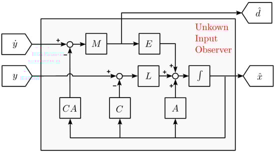
Figure 1.
UIO block diagram.
It is important to notice that the observer Equation (6) requires the knowledge of , which may pose challenges due to the need to differentiate the measurements, especially when noise is significant.
Having defined the matrix as:
the observer dynamics is then governed by the following equation:
Therefore, the second condition for the existence of the UIO is that the couple of matrices is detectable. Finally, the gain matrix can be defined according to different approaches, such as pole placement or optimal observer techniques.
An alternative formulation of Equation (8) is obtained by introducing a new state vector:
Accordingly, the observer dynamics becomes:
where the matrix is defined as:
In this way, the estimation of the state vector can be obtained without directly differentiating the measurement vector . However, the computation of the disturbance through Equation (5) still requires a differentiation step.
In summary, this section presents the governing equations of the UIO algorithm. In the present study, the general algorithm is applied to reconstruct the track geometry, namely, the disturbance acting on the system, based on the available measurements and the knowledge of the dynamic model of the railway vehicle.
3. Application of the UIO for the Estimation of the Track Vertical Alignment
In this section, the procedure followed to apply the UIO algorithm targeting the identification of railway track geometry is presented. At this stage of the research, a commercial vehicle equipped with inertia sensors was not available. Therefore, as described in Figure 2, simulations using Simpack multibody software are adopted.
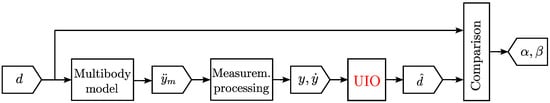
Figure 2.
Validation strategy of the UIO algorithm through multibody simulations performed with Simpack.
In the simulations, known irregularities (acting as disturbances ) are introduced as external excitations to generate bogie and carbody accelerations (denoted as ), which are processed to obtain the measurements required as inputs of the UIO algorithm (). Finally, the track geometry estimation is compared to the input of the multibody model . In the considered application, major attention is, in fact, placed on the identification of the disturbance , which represents the mean vertical alignment of the track.
To determine the accuracy reached by the proposed estimation algorithm, we propose two indices, and , that will be extensively introduced in Section 4. In Section 3.1 the vehicle model considered in this work is presented. Secondly, in Section 3.2 two simulation scenarios are described, respectively, considering the vehicle running along straight and curved tracks at constant speed.
3.1. Generation of Measurements Through Multibody Simulations
The vehicle model adopted in this research to generate the measurements data required to test the UIO algorithm is the well-known Manchester Benchmark model. The reference vehicle is the Vehicle 1, reported in [33], based on the ERR1 B176 benchmark vehicle. This railway vehicle has been completely modelled in the commercial multibody software Simpack, considering the nonlinearities of the system. The operating scenarios analysed in this work are the following:
- straight track, with the vehicle running at 160 km/h;
- curved track, with the radius of 1000 m and the track cant equal to 90 mm, with the vehicle running at 140 km/h, resulting in a cant deficiency of 150 mm. The track layout is reported in Figure 3 for clarity.
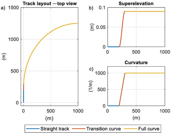 Figure 3. Track layout considered for the curved scenario. (a) top view; (b) superelevation; (c) curvature.
It is worth remarking that the assumption of constant speed was considered in this work. On the one hand, this is a reasonable choice to test the performance of the UIO algorithm at simulation stage, also on account of the considered vehicle, that is a general passenger coach [33] travelling at constant speed. On the other hand, in real-case scenarios, slight speed variations would also be expected when considering a track section carried out at nominal constant speed (for instance, due to fluctuations in line gradient). In any case, in Section 5 a sensitivity analysis of the UIO performance considering different vehicles’ speed will be presented.
Concerning the track geometry, longitudinal level, alignment, and cross-level components can be introduced in the numerical simulations as external excitations to the railway vehicle, to closely replicate real-world conditions. The power spectral density (PSD) function of ERRI B176 [34] is used to generate the track geometry (large defects), which are reported in Figure 4. As later described, different simulations have been analysed, considering either the sole longitudinal level profile of Figure 4a as input of the simulations, or contemporarily activating all the geometry components of Figure 4. The latter case is meant to be a more realistic scenario; however, it is here anticipated that the attention will be still paid only to the identification of the track mean vertical profile (mean value between the longitudinal level recorded on individual rails), that is the track geometry parameter of interest in this work.
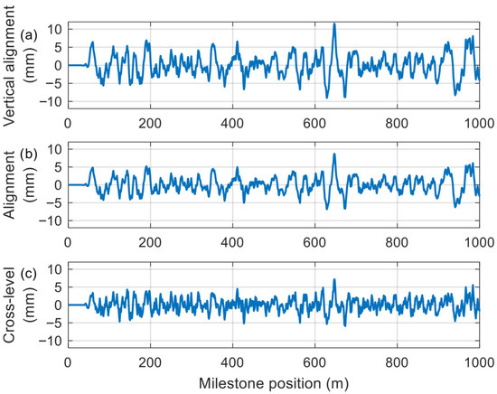
Figure 4.
Track geometry components generated adopting the PSD from ERRI B176 (large defects), wavelengths: 1–70 m. (a) vertical alignment, (b) lateral alignment, (c) cross-level. It is worth noting that track components are set to null values in the initial 50 m, in order to properly set initial conditions to the simulations.
For the sake of completeness, it should be noted that the track was considered as rigid, thus not including its flexibility nor elastic supports. Although this is a simplification, it is aligned with the frequency range of interest of this study (0–15 Hz, coherently with the track defect wavelength of 1–70 m). In fact, in this frequency range, ballast tracks do not show any amplifications associated with their dynamics. By contrast, in case shorter wavelengths would be considered (for example, in case of rail corrugation or roughness), it is then expected that the role of track flexibility will have a significant impact on the vehicle response, thus requiring a more refined modelling strategy to run the Simpack simulations.
Finally, using the multibody model of the Manchester Benchmark vehicle 1 [33], the bogie accelerations are adopted to feed the proposed UIO algorithm, enabling the reconstruction of the time history of the irregularities used as inputs for the simulations.
3.2. Reference Vehicle Model for Vertical Track Profile Estimation
Finally, in this work, the UIO algorithm is adopted, aiming at the estimation of the mean vertical railway track profile. Since UIO is a model-based algorithm, a simplified model of a rail vehicle (based on the Manchester Benchmark parameters) in the vertical plane is required. The scheme of the vehicle model employed is reported in Figure 5. This model considers seven rigid bodies as follows: one carbody, two bogie, and four wheelsets connected by means of primary and secondary suspensions. The vehicle model includes the vertical displacements and pitch rotations of the carbody, the leading and the trailing bogies, resulting in a total of six degrees of freedom (DOFs), which are highlighted with red arrows in Figure 5. Primary and secondary suspensions are modelled as linear springs and dampers in parallel, acting both along the vertical and the longitudinal directions.
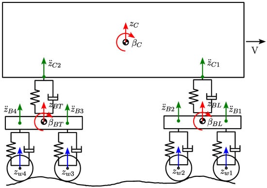
Figure 5.
Railway vehicle model—red arrows represent the degrees of freedom, green arrows represent vertical sensor measurements, whilst blue arrows represent the disturbances (vertical track irregularities) of the system.
As already mentioned, using as independent variable the vector , collecting the vertical displacements of bogies and carbody together with their pitch rotations (indicated with red arrows in Figure 5), is defined as:
The equations of motion of the mechanical system can be written in state space formulation. In this form, the state vector collects the vector and its time derivative as:
while and represent the vectors of the disturbances, which are the displacements of the wheelsets and their time derivatives (indicated with blue arrows in Figure 5). In fact, the modelling assumption is that the vertical displacement of the axleboxes corresponds exactly to the vertical alignment of the rail, which is to be estimated. Thus, it is possible to write the following equation:
Since and are not independent disturbances (the latter being the time derivative of the former), the state vector can be augmented to include :
It is then possible to rewrite the state equation as:
Additionally, it is possible to relate the vertical displacement of the k-th wheelset to the one of the i-th wheelset by accounting for time delay , which depends on the distance between the two considered wheelsets and the vehicle speed:
In the Laplace domain, the time delay corresponds to multiplication by an exponential function:
Assuming a small delay, the exponential function in the Laplace domain can be approximated by a rational function using the so-called Padé approximation. If a second order approximation is used, the following expression holds:
This transfer function can be converted into a state space form by introducing two additional states for each wheelset:
Since the vehicle speed considered in this application is relatively low, the time delay between the first wheelset and the fourth wheelset falls within the range of 0.5 s, which is quite high. In order to increase the accuracy of Padé approximation for such long delays, higher order approximations are typically required. However, this solution would lead to significantly larger number of states for the overall system. As a result, observability and detectability issues for the system matrices can rise, compromising the applicability of the methodology. Alternatively, it is possible to treat the inputs on the leading wheelsets of the leading and trailing bogies as independent and model the inputs on the trailing wheelsets as delayed versions of these.
As a result, Padé approximation is applied only to the second and fourth wheelset of the vehicle. Consequently, two additional groups of states and must be introduced when rewriting Equation (16). Using the following augmented state vector:
and the disturbance vector:
the system dynamics can be expressed as:
which has the same structure as the state equation reported in Equation (1), with a zero-input vector u.
To summarise, the UIO leverages a vehicle model characterised by an augmented state vector composed of 20 state variables, detailed as follows:
- 12 states corresponding to the independent coordinates and their time derivatives, grouped in the vector xm;
- 4 states accounting for the wheelset displacement inputs, represented by the vectors . These states are included to enable the estimation of the time derivatives which act as system inputs;
- 4 states and arising from the second-order Padé approximation used to represent the time delay between the inputs acting on the first and third wheelsets, and those on the second and fourth wheelsets.
As far as the measurement vector y and its time derivative are concerned, they can be obtained by integrating the acceleration measurements.
Considering this model, to satisfy the necessary condition for the observability of the disturbances expressed in Section 2, a minimum of four measurements should be available to reconstruct the vertical irregularity of the track. These measurements must be associated with the motion of the bogies. Additionally, to improve the accuracy of the estimation, measurements on the carbody are also included. Therefore, as the final configuration, it is assumed to measure two vertical accelerations on each bogie and two on the carbody, resulting in a total of six sensors, depicted as green arrows in Figure 5.
The acceleration measurements performed on the vehicle can be seen as a linear combination of the derivatives of the state variables:
The vectors and in input to the UIO can be defined considering the vector of the acceleration measurements and its first and second time integrals, according to
The vector , therefore, is given by:
The matrix, to be used in the measurement equation, is then obtained from Equation (26) by introducing columns of zeros to conform to the dimension of vector
Finally, the gain matrix is derived as the optimal solution to a continuous-time algebraic Riccati equation.
4. Results of the Identification
For the sake of brevity, only a selection of representative results is presented in this work, referring to the simulations described in Section 3.1. It is recalled that two simulations are considered, respectively, carried out along a straight track (with the vehicle running at 160 km/h) and along a curved track (curve radius of 1000 m run at 144 km/h). In the latter case, the analysis is restricted to the full curve condition, i.e., after the transition curve is completed. It is also noted here that, to test the performance of the UIO algorithm, the assumption of constant travelling speed was made at this stage. In the research follow-up, the possibility of also including speed variation can be explored by defining suitable gain matrices L for different speed ranges, according to the gain scheduling technique.
At first, in Section 4.1, the focus is on Simpack simulations performed considering only the vertical track profile as input (as shown in Figure 4a). Both simulations, along the straight and curved tracks, are considered. Then, in Section 4.2, the same Simpack simulations along straight and curved track are re-analysed, this time contemporarily considering vertical, lateral, and cross-level irregularities as inputs. This choice is meant to define a more realistic simulation by including all track geometry components that typically affect the railway track. In all the considered cases, noise is added to the measured data (vehicle carbody and bogie accelerations). To do so, reference is made to commercial MEMS low-noise sensors available on the market. Specifically, Table 1 shows the characteristics of the sensors considered to include noise disturbance at the processing stage.

Table 1.
Sensors’ characteristics adopted to introduce noise contribution to the bogie and carbody acceleration.
The noise density values reported in Table 1 are assumed as target root mean square values to be added to the simulated accelerations. To reproduce the desired characteristics, a Gaussian noise was first generated; low pass filtering with a cutoff frequency was applied (in accordance with the technical datasheet of the sensors); finally, to respect the desired characteristics, the noise was scaled according to
The generated noise was added to the corresponding acceleration signals. It is here specified that two different realisations of noise signal were considered for the carbody accelerations (front and rear carbody ends), while eight noise signals were generated for bogie sensors (four for the front and four for the rear bogies). Noisy accelerations were then processed to determine the inputs of the UIO algorithm (for instance, carbody and bogies pitch accelerations, etc.).
It is here recalled that, in all the cases considered both in Section 4.1 and Section 4.2, the aim is the identification of exclusively the mean vertical track profile adopting the UIO algorithm. As it will be shown in the next sections, the proposed simplified railway vehicle model is able to fulfil the task. On the other hand, being an in-plane model, it is not suitable for identifying the longitudinal level of individual rails, as well as the cross-level irregularity component. This is, in fact, the first attempt to apply the UIO algorithm to the railway track profile estimation, while future work will focus on the identification of other track geometry components such as longitudinal level (individual rails), alignment, and cross-level.
4.1. Simulations Performed Considering as Input Only the Vertical Track Irregularity
Figure 6 shows the results of the identification for the straight track simulation, in the case where only vertical track irregularity is considered. The input track irregularity is depicted as a blue line, while the one identified by the UIO algorithm is shown as a red line. Specifically, Figure 6a presents the results obtained from the estimation of input at the leading wheelset of the leading bogie, while in Figure 6b those from the leading wheelset of the trailing bogie are presented. The data have been aligned by taking into account the pivot pitch of the vehicle (equal to 19 m), so as to represent the same track irregularity as a function of the milestone position.
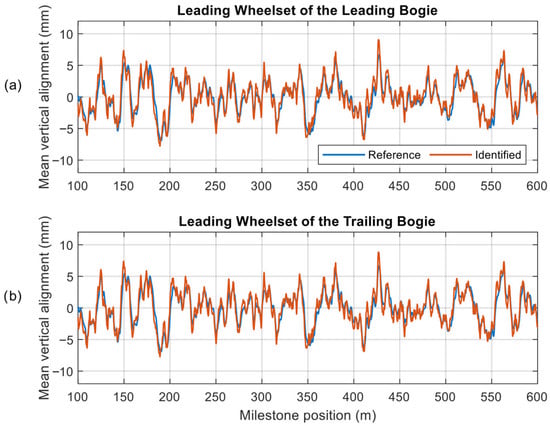
Figure 6.
Comparison between the reference vertical alignment and the one estimated by the UIO algorithm. Signal histories of the input at (a) leading wheelset of the leading bogie and (b) leading wheelset of the trailing bogie, as a function of the milestone position. Simulation along straight track at 160 km/h, considering only vertical track irregularity as input.
Comparing the reference and the identified track profiles, a satisfactory agreement can be observed for both bogies, the two lines being almost superimposed. However, an overestimation can be observed in some of the irregularity peaks.
To further analyse the results, the frequency components of the signal were analysed, as reported in Figure 7. It can be noted that while the low-frequency content is well identified, an overestimation is evident in the 3–10 Hz range, which explains the signal histories of Figure 6. This discrepancy may be related to the weights considered in the definition of the gain matrix of the UIO algorithm but can still be considered as promising, as they prove the model capability to identify the track irregularity.
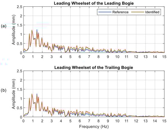
Figure 7.
Comparison between the reference vertical alignment and the one estimated by the UIO algorithm. Spectra of the input at the (a) leading wheelset of the leading bogie and (b) leading wheelset of the trailing bogie. Simulation along straight track at 160 km/h, considering only vertical track irregularity as input.
Since the model employed in the UIO has two external disturbances, as written in Equation (22), the proposed procedure provides two separate estimations of the track irregularity, which are in strong agreement both in terms of time histories and spectral components. However, a unique track profile is actually responsible for the dynamic response of the vehicle, as confirmed by the blue lines in Figure 6 and Figure 7, which are coincident. Therefore, a final step of post-processing is required to obtain a unique estimation of the track profile.
The data, reported as a function of the milestone position, allow for averaging the estimations of vertical irregularity, followed by the computation of the corresponding spectrum. The result of the averaging procedure is shown in Figure 8, which represents the final outcome of the application of the UIO algorithm (defined as ‘irregularity estimation’ in Table 2).

Figure 8.
Comparison between the reference vertical alignment and the one estimated by the UIO algorithm. (a) Signal history and (b) spectrum of the average signals. Simulation along straight track at 160 km/h, considering only vertical track irregularity as input.
Table 2.
Identification indexes, considering only vertical track irregularity as input of the simulations.
To quantify the degree of accuracy achieved by the identification, and to further validate the results presented in Figure 6 through Figure 8, two synthetic indices are proposed. They are denoted as and , respectively, and are used to assess the overall consistency of the results, both in the time and frequency domains. For the time domain, the normalised squared error defined in Equation (29) is employed, where a zero index means perfect estimation A similar index is proposed for the frequency domain, with the error evaluation based on the differences in spectral intensity, as described in Equation (30).
Table 1 shows the results of the two indices expressed as percentages. For the considered straight track simulation, the α index is equal to 13.2% and 12.2% when the identification is performed considering the accelerations from, respectively, the leading and the trailing bogies. If the average is considered, a value of 12.5% is obtained, showing a good agreement between the estimated irregularity and the actual one, in all the considered cases. The α index takes into account not only the magnitude of the irregularity, but also its position along the line. Therefore, a small delay of the reconstructed signal, which from a practical point of view would not be a significant issue, generates a worsening of the index. The second index β instead focuses on the capacity of the observer to reconstruct the magnitude of the different wavelengths present in the irregularity. The index β assumes a value of 4.1% and 4.0% for the two bogies, and an average value of 3.9%, showing how the observer is able to estimate the spectral content of the irregularity with a high degree of accuracy.
Once the straight track simulation has been analysed, attention is shifted to the simulation performed along the curved track (see Section 3.1). For the sake of brevity, only the final results (after the averaging of the two track profiles identified, as for the straight track scenario) are shown in Figure 9. Specifically, Figure 9a shows the comparison of the signal histories, while in Figure 9b, the frequency domain analysis is presented. It is worth mentioning that the considered portion of the track refers to a full curve (i.e., the transition curve is excluded from the analysis).
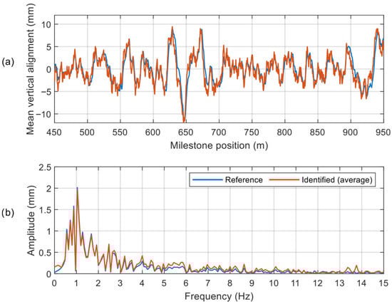
Figure 9.
Comparison between the reference vertical alignment and the one estimated by the UIO algorithm. (a) Signal history and (b) spectrum of the average signals. Simulation along curved track (after transition curve) at 144 km/h, considering only vertical track irregularity as input.
Also in this case, a satisfactory agreement between the reference and identified track profile can be observed, both in terms of signal histories and spectral content, although similar comments to those made for Figure 8 can be applied.
To conclude the analysis of the curved simulation, the and coefficients are computed and reported in Table 2. It can be observed that is characterised by an increase compared to the straight track case. The best estimation is reached in the case of averaged signals, with assuming a value of 17.6%. Conversely, assumes an average value of 3.3% which is even lower than the one reached in the straight track case. Despite the overestimation at 13–14 Hz previously described, the identified spectrum is, in fact, representing the frequency content of the actual track profile well, thus confirming the capability of the UIO algorithm to identify the track vertical alignment.
4.2. Simulations Performed Considering as Input Vertical, Lateral, and Cross-Level Track Geometry Components
In this section, the same scenarios are re-analysed considering a more realistic representation of track. In detail, all the geometry components (vertical, lateral, and cross-level) were simultaneously introduced in Simpack simulations, as described in Section 3.1. The UIO algorithm was then applied to reconstruct the track vertical profile, using the same in-plane vehicle model shown in Figure 5. In fact, alignment and cross-level irregularities were included only to reproduce a more realistic vehicle response in Simpack simulations, while the UIO identification remains focused on the vertical track component. Therefore, the two additional irregularity components are unmodelled disturbances, that can be seen as “noise-like” contributions to the main objective of the study. It actually turns out that these additional track components play a much more important role in the quality of the identification, compared with the noise contributions affecting the measurements.
At first, straight track simulation is considered, as shown in Figure 10, according to the same data representation. It is worth noting that no significant difference can be observed with respect to the simplified case presented in Figure 8 (where simulations were run considering only vertical irregularity as input). In fact, both the signal history of the track profile and the corresponding spectrum are still well identified by the algorithm.
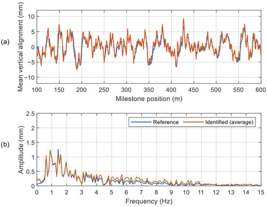
Figure 10.
Comparison between the reference vertical alignment and the one estimated by the UIO algorithm. (a) Signal history and (b) spectrum of the average signals. Simulation along straight track at 160 km/h, simultaneously considering vertical, lateral, and cross-level irregularities as inputs.
This outcome is also confirmed by the α and β coefficients reported in Table 3, which in the case of averaged results assume values of 14.6% and 4.9%, respectively. Minor increases (in the order of 2% and 1%) are observed if the results of Table 3 are compared to those of Table 2, further confirming the capability of the UIO algorithm to identify the track irregularity even in more realistic scenarios.
Table 3.
Identification indexes. considering vertical, lateral, and cross-level irregularities as inputs of the simulations.
Finally, the curved track simulation was re-analysed and presented in Figure 11. In this case, the comparison between the actual and identified track profiles shows less accurate results, with some overestimation of the irregularity defects. For example, α and β assume values of 28.7% and 10.1%, respectively, for the averaged track irregularity. If reference is made to the spectrum of the signal, it is evident that the low-frequency contribution (up to 3 Hz) is well identified by the algorithm; conversely, a pervasive overestimation in the 3–12 Hz frequency range is observed. This result was to some extent expected, given the dynamic amplification that may occur when negotiating a curve if different types of track irregularities are forcing the rail vehicle. For instance, to explain the lower performance of the UIO identification, reference can be made to the non-linear contributions (present in the Simpack model adopted to generate the data) that are not considered by the simplified rail vehicle model adopted by the UIO algorithm. Further analyses are proposed in the following Section 5, considering also a different curve radius. However, the outcome is still promising, confirming the feasibility to identify the track vertical alignment in all the considered cases. To improve the quality of the results, the option of refining the selection of the weights of gain matrix of the UIO algorithm could also be explored.
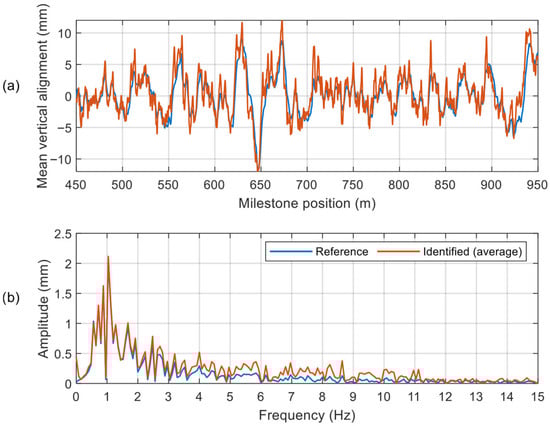
Figure 11.
Comparison between the reference vertical alignment and the one estimated by the UIO algorithm. (a) Signal history and (b) spectrum of the average signals. Simulation along curved track (after transition curve) at 144 km/h, simultaneously considering vertical, lateral, and cross-level irregularities as inputs.
5. Robustness of the UIO Algorithm
In this section, the robustness of the UIO algorithm is analysed. The model adopted in the UIO algorithm is a reduced order model and can be affected by different uncertainties, possibly related to unknown parameters, suspension non-linearities, or measurements noise. Therefore, to assess the reliability of the proposed algorithm in terms of the α and β indices, a set of new multibody simulations are hereafter proposed. To test the UIO performance, the parameters of the in-plane model adopted for the vertical alignment identifications are kept constant throughout all simulations, as is the gain matrix of the observer.
Both straight and curved tracks are considered, taking into account vertical, lateral, and cross-level irregularities as inputs of the simulations. At first, attention is given to the uncertainty in vehicle parameters, considering cases a and b as hereafter described.
- Case a.1 and a.2: 20% increase and decrease in the vehicle mass. This parameter varies mainly due to changes in the number of passengers occupying the vehicle.
- Case b.1 and b.2: two different random realisations of primary suspension stiffness are generated, deviated from the nominal value according to a Gaussian distribution. A ± 20% variation, corresponding to a 3σ range, is considered. This parameter variation is introduced to account for the statistical variability in the stiffness of the components of the primary vertical suspension.
In addition, the influence of vehicle speed and track layout on the results is investigated, considering the following simulations (assuming nominal mass and stiffness parameters):
- Case c: straight track simulation with the vehicle running at 100 km/h;
- Case d: curved track simulation considering a radius of 420 m and a track cant of 150 mm, with the vehicle running at 104 km/h, resulting in a non-compensated condition.
Finally, the effect of sensors’ noise is analysed. It is noted here that simulations presented in Section 4.1 and Section 4.2 already include noise affecting both carbody and bogie accelerations.
- Case e: tenfold increase in noise density affecting both bogie and carbody accelerations. Simulations along both straight track (160 km/h) and curved track (144 km/h) are considered.
The and coefficients resulting from cases a–e are reported in Table 4, considering the final outcome of the UIO identification (average track irregularity only). For comparison, the nominal case presented in Section 4.2 is also reported.
Table 4.
Robustness analysis of the UIO algorithm considering vertical, lateral, and cross-level irregularities as inputs of the simulations. Case a.1: increase of 20% the mass carbody—Case a.2: decrease of 20% of the vehicle mass—Case b.1 and b.2: primary suspension stiffness deviations from the nominal value—Case c: straight track scenario with the vehicle running at 100 km/h—Case d: curved track with a radius of 420 m and a track cant of 150 mm, with the vehicle running at 104 km/h—Case e: tenfold increase in noise contribution of bogie and carbody accelerations, applied to the nominal case.
Referring to Table 4, the variation in the carbody mass (case a.1 and a.2) shows a small influence on the UIO performance, with deviations of α and β in the order of 4% and 2%, respectively. Similar results are also achieved considering the effect of primary suspension stiffness (see case b.1 and b.2). These results demonstrate the robustness of the proposed UIO algorithm to cope with the vehicle parameters’ uncertainty.
Changing the vehicle speed along a straight track (case c) leads to minor variations as well, with negligible fluctuations of α and a minor increase (in the order of few percent) for β. Conversely, significant differences can be observed in curved track scenarios. In particular, case (d) considers the negotiation of a sharp curve of 420 m radius, which brings to a worsening of the α index of about 12%. Given this significant variation, an in-depth analysis of the scenario was carried out. The multibody simulation (case d) shows that negotiating a curve with such a small radius causes the lateral bump stops to come into contact with the carbody, introducing an additional non-linear stiffness effect. This non-linearity is not captured by the simplified in-plane vehicle model used in the UIO algorithm, which can explain its reduced accuracy in reconstructing the mean vertical alignment. Furthermore, other vehicle non-linearities could also influence the estimation results.
Finally, the effect of signal noise is analysed with reference to case e. From Table 4, it is apparent that the tenfold increase in noise density (on both carbody- and bogie-mounted sensors) does not affect the results in terms of and indexes. Upon further investigation, it was verified that variations smaller than 0.1% are actually obtained (thus not visible in Table 4) when the indexes computed by averaging the reconstructions from leading and trailing bogies are considered. Conversely, if the reconstructions from the single bogies are considered, the and variations remain on the order of 1%. The final outcome (reported in Table 4, and unaffected by the increase in noise contribution) therefore benefits the averaging procedure, which reduces the detrimental effect of measurement noise. To complete the discussion on noise contribution, it is worth mentioning that in a real-case scenario, other sources of noise may arise within the overall measurement chain, potentially affecting the final estimation. However, these sources are difficult to quantify and were therefore excluded from the analysis, which only accounts for sensor noise.
6. Conclusions
In this paper, an application of the UIO algorithm to identify the railway track vertical alignment is presented. First, the working principles of the algorithm were outlined, with a focus on the features tailored for the identification of railway track profile. Since an instrumented vehicle with the necessary equipment was not available at this stage of the research, the required data were generated via a vehicle dynamic simulation in Simpack, using the Manchester Benchmark vehicle model.
Two reference simulations were used to evaluate the UIO algorithm: a vehicle running at constant speed along both straight and curved tracks. Primary attention was devoted to estimating the mean vertical track alignment, which is critical for railway safety. To this end, carbody and bogie acceleration signals served as inputs for the UIO algorithm.
For each simulation, two different scenarios in terms of input geometry were tested. Initially, only the vertical alignment was considered. Subsequently, the simulations were re-analysed simultaneously including three track geometry components, namely vertical, lateral, and cross-level. In all simulations, signal noise contribution is included considering typical sensors installed on railway vehicles.
The validation of the results was performed by comparing the reference and estimated track vertical alignment both in terms of signal histories and spectral components, introducing the α and β synthetic indices (the lower the index, the better). In all the considered cases, the comparison shows satisfactory results, which are briefly summarised below:
- straight track simulations showed the most promising results. The α and β indices assume values of 12.5% and 3.9% when the simplified scenario with only vertical irregularity is considered. Slight increases were observed when all track irregularity components were activated, leading to 14.6% and 4.9%, respectively;
- curved track simulations are affected by larger estimation errors, with α and β coefficients equal to 28.7% and 10.1%, respectively.
In addition, results from robustness and sensitivity analyses have been included to evaluate the performance of the UIO algorithm under variations in model parameters, vehicle speeds, track geometries, and measurement noise. Specifically, variations in the carbody mass (±20%), primary suspension stiffness, and vehicle speed were tested, as well as the addition of Gaussian noise representative of commercial MEMS accelerometers, including a tenfold increase in noise density.
The results indicate that, for straight track scenarios, the and indices remain below 19% and 8%, respectively, even under parameter variations and increased noise. For curved tracks, the α index increases in the sharpest curve scenario, while the index remains below 13%. The reduction in performance for sharp curves is primarily due to the contact between the carbody and the lateral bump stops, which introduces additional non-linear stiffness effects not captured by the simplified in-plane vehicle model. On the other hand, no significant effect related to sensors’ noise was observed, even if in a real-case application the overall measurement chain may introduce additional noise contributions.
Overall, these analyses confirm that the UIO algorithm maintains satisfactory estimation accuracy and robustness in the presence of realistic uncertainties and sensor noise, highlighting its potential applicability to real-world railway track monitoring and providing a quantitative basis for future improvements. However, the current implementation of the proposed UIO algorithm is not suitable for identifying the longitudinal level of individual rails or other track geometry components, such as cross-level and alignment, which would require a higher model complexity. In addition, to further enhance estimation accuracy, the refinement of the weighting selection used in computing the observer gain matrix could be investigated.
Ultimately, the UIO algorithm has proven to be a promising tool for model-based track identification. In the project follow-up, attention will be given to these additional contributions to track geometry, also foreseeing the possibility to include the effect of speed variability through the gain-scheduling technique. In addition, future work could apply the algorithm to real-world data from an instrumented vehicle to further validate its performance.
Author Contributions
Conceptualization, S.A., M.S., I.L.P., E.D.G. and A.F.; methodology, S.A., E.D.G. and A.F.; software, S.A., M.S., I.L.P. and E.D.G.; validation, S.A., M.S., I.L.P. and E.D.G.; formal analysis, S.A., M.S., I.L.P., E.D.G. and A.F.; investigation, S.A., M.S., I.L.P. and E.D.G.; resources, E.D.G. and A.F.; writing—original draft preparation, M.S., I.L.P. and E.D.G.; writing—review and editing, S.A., M.S., I.L.P., E.D.G. and A.F.; visualisation, S.A., M.S., I.L.P. and E.D.G.; supervision, S.A., E.D.G. and A.F.; All authors have read and agreed to the published version of the manuscript.
Funding
This study was carried out within the MOST—Sustainable Mobility National Research Centre and received funding from the European Union Next-GenerationEU (PIANO NAZIONALE DI RIPRESA E RESILIENZA (PNRR)—MISSIONE 4 COMPONENTE 2, INVESTIMENTO 1.4—D.D. 1033 17/06/2022, CN00000023).
Institutional Review Board Statement
Not applicable.
Informed Consent Statement
Not applicable.
Data Availability Statement
The data presented in this study are available in the article.
Conflicts of Interest
The authors declare no conflicts of interest.
Abbreviations
The following abbreviations are used in this manuscript:
| UIO | Unknown Input Observer |
| TRV | Track Recording Vehicles |
| KF | Kalman Filter |
| DOF | Degree Of Freedom |
| PSD | Power Spectral Density |
References
- EN 13848-5:2017; Railway Applications—Track—Track Geometry Quality. Part 5: Geometry Quality Levels—Plain Line, Switches and Crossings. European Standard: Brussels, Belgium, 2017.
- Weston, P.; Roberts, C.; Yeo, G.; Stewart, E. Perspectives on Railway Track Geometry Condition Monitoring from In-Service Railway Vehicles. Veh. Syst. Dyn. 2015, 53, 1063–1091. [Google Scholar] [CrossRef]
- Rosano, G.; Massini, D.; Bocciolini, L.; Zappacosta, C.; Di Gialleonardo, E.; Somaschini, C.; La Paglia, I.; Pugi, L. Diagnostics of the railway track-Possibility of development through the measurement of accelerations and contact forces La diagnostica dell’armamento ferroviario—Possibilità di sviluppo attraverso la misura di accelerazioni e forze di contatto. IF 2024, 79, 81–102. [Google Scholar] [CrossRef]
- Baasch, B.; Roth, M.; Groos, J.C. In-Service Condition Monitoring of Rail Tracks. Int. Verkehrswesen 2018, 70, 76–79. [Google Scholar] [CrossRef]
- Fernández-Bobadilla, H.A.; Martin, U. Modern Tendencies in Vehicle-Based Condition Monitoring of the Railway Track. IEEE Trans. Instrum. Meas. 2023, 72, 1–44. [Google Scholar] [CrossRef]
- La Paglia, I.; Carnevale, M.; Corradi, R.; Di Gialleonardo, E.; Facchinetti, A.; Lisi, S. Condition Monitoring of Vertical Track Alignment by Bogie Acceleration Measurements on Commercial High-Speed Vehicles. Mech. Syst. Signal Process. 2023, 186, 109869. [Google Scholar] [CrossRef]
- La Paglia, I.; Di Gialleonardo, E.; Facchinetti, A.; Carnevale, M.; Corradi, R. Acceleration-Based Condition Monitoring of Track Longitudinal Level Using Multiple Regression Models. Proc. Inst. Mech. Eng. Part F J. Rail Rapid Transit 2024, 238, 479–488. [Google Scholar] [CrossRef]
- La Paglia, I.; Di Gialleonardo, E.; Facchinetti, A.; Carnevale, M.; Corradi, R. A Methodology to Estimate Railway Track Conditions from Vehicle Accelerations Based on Multiple Regression. In Proceedings of the Experimental Vibration Analysis for Civil Engineering Structures; Limongelli, M.P., Giordano, P.F., Quqa, S., Gentile, C., Cigada, A., Eds.; Springer Nature: Cham, Switzerland, 2023; pp. 203–210. [Google Scholar]
- Zanelli, F.; La Paglia, I.; Debattisti, N.; Mauri, M.; Tarsitano, D.; Sabbioni, E. Monitoring Railway Infrastructure Through a Freight Wagon Equipped with Smart Sensors. In Proceedings of the Experimental Vibration Analysis for Civil Engineering Structures; Limongelli, M.P., Giordano, P.F., Quqa, S., Gentile, C., Cigada, A., Eds.; Springer Nature: Cham, Switzerland, 2023; pp. 193–202. [Google Scholar]
- La Paglia, I.; Araya Reyes, C.E.; Di Gialleonardo, E.; Facchinetti, A.; Carnevale, M. A Speed-Dependent Condition Monitoring System for Track Geometry Estimation Using Inertial Measurements; National Research Council Canada: Ottawa, ON, Canada, 2023. [Google Scholar]
- Westeon, P.F.; Ling, C.S.; Roberts, C.; Goodman, C.J.; Li, P.; Goodall, R.M. Monitoring Vertical Track Irregularity from In-Service Railway Vehicles. Proc. Inst. Mech. Eng. Part F J. Rail Rapid Transit 2007, 221, 75–88. [Google Scholar] [CrossRef]
- Tsunashima, H.; Naganuma, Y.; Kobayashi, T. Track Geometry Estimation from Car-Body Vibration. Veh. Syst. Dyn. 2014, 52, 207–219. [Google Scholar] [CrossRef]
- Bocciolone, M.; Caprioli, A.; Cigada, A.; Collina, A. A Measurement System for Quick Rail Inspection and Effective Track Maintenance Strategy. Mech. Syst. Signal Process. 2007, 21, 1242–1254. [Google Scholar] [CrossRef]
- Bruni, S.; Carnevale, M.; Cazzulani, G.; Di Gialleonardo, E.; La Paglia, I. AI for Rail Infrastructure and Maintenance. In Handbook on Digital Twin and Artificial Intelligence Techniques for Rail Applications; CRC Press: Boca Raton, FL, USA, 2025. [Google Scholar]
- Hadj-Mabrouk, H. Contributions and Limitations of AI and Machine Learning in Railway Operations, Maintenance, and Safety: A Literature Review. Proc. Inst. Mech. Eng. Part O J. Risk Reliab. 2025, 1748006X251364324. [Google Scholar] [CrossRef]
- Helmi, W.; Bridgelall, R.; Askarzadeh, T. Remote Sensing and Machine Learning for Safer Railways: A Review. Appl. Sci. 2024, 14, 3573. [Google Scholar] [CrossRef]
- Gibert, X.; Patel, V.M.; Chellappa, R. Deep Multitask Learning for Railway Track Inspection. IEEE Trans. Intell. Transp. Syst. 2017, 18, 153–164. [Google Scholar] [CrossRef]
- Hajizadeh, S.; Núñez, A.; Tax, D.M.J. Semi-Supervised Rail Defect Detection from Imbalanced Image Data. IFAC-Pap. 2016, 49, 78–83. [Google Scholar] [CrossRef]
- Chenariyan Nakhaee, M.; Hiemstra, D.; Stoelinga, M.; van Noort, M. The Recent Applications of Machine Learning in Rail Track Maintenance: A Survey. In Proceedings of the Reliability, Safety, and Security of Railway Systems. Modelling, Analysis, Verification, and Certification, Lille, France, 4–6 June 2019; Collart-Dutilleul, S., Lecomte, T., Romanovsky, A., Eds.; Springer International Publishing: Cham, Switzerland, 2019; pp. 91–105. [Google Scholar]
- Alfi, S.; Bruni, S. Estimation of Long Wavelength Track Irregularities from on Board Measurement. In Proceedings of the 2008 4th IET International Conference on Railway Condition Monitoring, Derby, UK, 17–20 June 2008; pp. 1–6. [Google Scholar]
- Alfi, S.; De Rosa, A.; Bruni, S. Estimation of Lateral Track Irregularities from On-Board Measurement: Effect of Wheel-Rail Contact Model. In Proceedings of the 7th IET Conference on Railway Condition Monitoring 2016 (RCM 2016), Birmingham, UK, 27–28 September 2016; IET: Stevenage, UK, 2016; p. 18. [Google Scholar] [CrossRef]
- De Rosa, A.; Alfi, S.; Bruni, S. Estimation of Lateral and Cross Alignment in a Railway Track Based on Vehicle Dynamics Measurements. Mech. Syst. Signal Process. 2019, 116, 606–623. [Google Scholar] [CrossRef]
- De Rosa, A.; Kulkarni, R.; Qazizadeh, A.; Berg, M.; Di Gialleonardo, E.; Facchinetti, A.; Bruni, S. Monitoring of Lateral and Cross Level Track Geometry Irregularities Through Onboard Vehicle Dynamics Measurements Using Machine Learning Classification Algorithms. Proc. Inst. Mech. Eng. Part F J. Rail Rapid Transit 2021, 235, 107–120. [Google Scholar] [CrossRef]
- Jensen, T.; Chauhan, S.; Haddad, K.; Song, W.; Junge, S. Monitoring Rail Condition Based on Sound and Vibration Sensors Installed on an Operational Train. In Proceedings of the Noise and Vibration Mitigation for Rail Transportation Systems, Terrigal, Australia, 12–16 September 2016; Nielsen, J.C.O., Anderson, D., Gautier, P.-E., Iida, M., Nelson, J.T., Thompson, D., Tielkes, T., Towers, D.A., de Vos, P., Eds.; Springer: Berlin/Heidelberg, Germany, 2015; pp. 205–212. [Google Scholar]
- Luenberger, D. An Introduction to Observers. IEEE Trans. Autom. Control. 1971, 16, 596–602. [Google Scholar] [CrossRef]
- Weston, P.F.; Ling, C.S.; Goodman, C.J.; Roberts, C.; Li, P.; Goodall, R.M. Monitoring Lateral Track Irregularity from In-Service Railway Vehicles. Proc. Inst. Mech. Eng. Part F J. Rail Rapid Transit 2007, 221, 89–100. [Google Scholar] [CrossRef]
- Lee, J.S.; Choi, S.; Kim, S.-S.; Park, C.; Kim, Y.G. A Mixed Filtering Approach for Track Condition Monitoring Using Accelerometers on the Axle Box and Bogie. IEEE Trans. Instrum. Meas. 2012, 61, 749–758. [Google Scholar] [CrossRef]
- Ding, S.X. Model-Based Fault Diagnosis Techniques: Design Schemes, Algorithms and Tools; Advances in Industrial Control; Springer: London, UK, 2013; ISBN 978-1-4471-4798-5. [Google Scholar]
- Mo, J.; Qin, D.; Liu, Y. Unknown Input Observer-Based Fault Diagnosis of Speed Sensors in Dual Clutch Transmission. Proc. Inst. Mech. Eng. Part D J. Automob. Eng. 2023, 237, 1710–1720. [Google Scholar] [CrossRef]
- Amrane, A.; Larabi, A.; Aitouche, A. Unknown Input Observer Design for Fault Sensor Estimation Applied to Induction Machine. Math. Comput. Simul. 2020, 167, 415–428. [Google Scholar] [CrossRef]
- Chen, J.; Patton, R.J. Robust Residual Generation Using Unknown Input Observers. In Robust Model-Based Fault Diagnosis for Dynamic Systems; Springer: Boston, MA, USA, 1999; pp. 65–108. [Google Scholar]
- La Paglia, I.; Santelia, M.; Alfi, S.; Di Gialleonardo, E.; Facchinetti, A. An Application of the Unknown Input Observer Algorithm for the Identification of Vertical Railway Track Irregularity. In Proceedings of the Railways 2024—The Sixth International Conference on Railway Technology: Research, Development and Maintenance, Prague, Czech Republic, 1–5 September 2024. [Google Scholar]
- Iwnick, S. Manchester Benchmarks for Rail Vehicle Simulation. Veh. Syst. Dyn. 1998, 30, 295–313. [Google Scholar] [CrossRef]
- UIC. ORE Power Spectral Density of Track Irregularities. In Part 1: Definitions, Conventions and Available Data; Question ORE C116-Rp1 1971; UIC Railway Publications: Paris, France, 1971. [Google Scholar]


Disclaimer/Publisher’s Note: The statements, opinions and data contained in all publications are solely those of the individual author(s) and contributor(s) and not of MDPI and/or the editor(s). MDPI and/or the editor(s) disclaim responsibility for any injury to people or property resulting from any ideas, methods, instructions or products referred to in the content. |
© 2025 by the authors. Licensee MDPI, Basel, Switzerland. This article is an open access article distributed under the terms and conditions of the Creative Commons Attribution (CC BY) license (https://creativecommons.org/licenses/by/4.0/).