A Unified Modelling Framework Combining FTA, RBD, and BowTie for Reliability Improvement

Featured Application

The proposed BowTie-based reliability framework provides a structured approach for examining and enhancing wind turbine resilience. It brings together preventive and mitigative pathways, enabling decision-makers, such as asset managers, to pinpoint critical barriers, prioritise maintenance, and evaluate the benefits of redundancy or redesign strategies. The methodology can also be applied to other critical infrastructure, particularly where critical processes are involved and defence-in-depth and quantitative risk justification are crucial. This makes the framework a practical decision-support tool for balancing multiple attributes, including safety, reliability, and cost, within complex engineered systems.

Abstract

Ensuring reliability and safety is essential in complex energy systems such as wind turbines, where failures can trigger unexpected downtimes, severe incidents, and significant costs. This study proposes a hybrid BowTie-based reliability framework that integrates Fault Tree Analysis, Reliability Block Diagrams, and BowTie methodology to quantify risk and evaluate the effectiveness of safety barriers. The framework employs key reliability metrics including availability, probability of failure on demand, and probability of failure per hour, and supports scenario-based sensitivity analyses to explore redesign options. A simulation-based case study of a wind turbine generator subsystem is presented, using parameter values drawn from published reliability data. Results highlight that protective relays and automatic trip systems represent critical single points of defence, while improvements such as enhanced oil analysis and redundant dashboards reduce consequence frequency from 2.912 × 10⁻¹⁷ to 8.257 × 10⁻¹⁹ failures/h (a 97.16% reduction, nearly two orders of magnitude). Compared to conventional models, the proposed framework introduces explicit defence in depth modelling, improves computational compactness, and provides a practical decision support tool for asset managers by balancing safety and reliability. At this stage, the study should be regarded as a proof of concept that demonstrates feasibility and sets a foundation for future research and application to larger, more complex infrastructures.

1. Introduction

Reliability analysis is an essential method in engineering that concentrates on the design, operation, and maintenance of complex systems, guiding maintenance strategies to improve asset performance. Traditional methods, such as Fault Tree Analysis (FTA) and Reliability Block Diagrams (RBDs), remain prevalent, offering structured approaches to identify failure logic and assess system performance. FTA, a top-down approach, uses Boolean logic to estimate failure probability, while RBD offers a complementary view at the system level, illustrating how components and subsystems interact through series and parallel configurations to ensure system functionality. Both techniques have proven effective in safety-critical fields such as nuclear power, aerospace, and energy infrastructure. Despite their long-standing usefulness, each has notable limitations when used alone [1,2]. FTA, although straightforward and rigorous, can become unwieldy in large systems due to combinatorial complexity and is limited by its static nature, which hampers its ability to model repair processes, time-dependent phenomena, or conditional interactions [3]. Conversely, RBD allows quick system-level insights but relies on binary assumptions, making it challenging to represent multi-state, dependent, or sequential behaviours. These constraints are particularly problematic in modern critical infrastructure, such as wind turbines (WT), where systems operate under dynamic conditions and exhibit interdependent failure modes.

Recent studies have attempted to overcome these limitations by hybridising FTA, RBD, and related methods. For example, Rivera et al. [4] suggest an integrated method that combines FTA, RBD, the Analytical Hierarchy Process (AHP), High Reliability Organisation (HRO), and Learning from Failures (LFF) tools to analyse long-term patterns of small to medium chronic failures in an Oil and Gas (O&G) organisation. However, this unified framework increases complexity and is sensitive to expert bias. Conversely, Kabir et al. [5] address individual limitations by assigning large, mainly series or parallel segments to a modularisation technique using Binary Decision Diagram (BDD) and Markov models. This approach can reduce the size and complexity of the embedded FTA, preventing the exponential growth of cut sets. Still, it requires advanced solvers and can make model traceability across modules challenging. Cheng et al. [6] share a similar viewpoint in their study on unified approaches, connecting FTA logic to a Hierarchical Belief Rule Base (BRB). They manage to mitigate issues related to excessive indexes and avoid combinatorial explosion [4], but the framework’s scalability remains unvalidated, and it has a limited domain focus.

Recent work has also explored hybrid frameworks that combine the BowTie method with probabilistic reasoning to overcome its static nature and expand its analytical capabilities. For example, Khakzad et al. [7] mapped a BowTie model into a Bayesian network to perform dynamic safety analysis. They noted that the BowTie approach remains popular for accident modelling but is limited by its static representation and inability to represent conditional dependencies. By translating the BowTie to a Bayesian network, probabilities can be updated in response to new information and causal relationships. Similarly, de Barnier et al. [8] introduce a possibility-based BowTie to quantify uncertainties in barrier performance. Another dynamic risk-assessment study [9] emphasises that BowTie is a visual method for depicting event progression from causes to effects, while a Bayesian network captures stochastic relationships. The translation from BowTie to Bayesian network modifies the representation to include intrinsic uncertainties while maintaining logical relationships. Although valuable, these unified methodologies often trade clarity for complexity, a lack of redundancy integration, and risk fragmentation in tool support across different methods [10]. The limitations of hybrid methods could lead to additional design and verification burdens affecting reproducibility and traceability. A comparative taxonomy of recent hybrid methods is summarised in Table 1, which positions the present work relative to state-of-the-art contributions.

Table 1. Comparative summary of hybrid reliability-modelling frameworks (2010–2024).

Study and Year	Hybrid Methods	Application Domain	Main Contribution
Rivera et al. (2021) [4]	FTA + RBD + AHP + HRO + Learning-from-Failures	Oil and Gas organisation	Multi-criteria framework linking organisational reliability factors with classic FTA/RBD models to analyse chronic failures
Kabir et al. (2020) [5]	Modular dynamic fault trees using BDD and Markov models	Safety-critical systems	Hybrid modularisation reduces state-space explosion in dynamic FTA, allowing non-exponential failure distributions
Cheng et al. (2023) [6]	FTA + Hierarchical Belief Rule Base (BRB)	Milling fault detection	Links FTA logic to a BRB to handle uncertainty and avoid combinatorial explosion
Khakzad et al. (2013) [7]	BowTie mapped to Bayesian network	Chemical process safety	Dynamic safety analysis by mapping BowTie to BN; allows update of probabilities and representation of conditional dependencies
de Barnier et al. (2022) [8]	Quantitative BowTie (possibility-based)	Industrial risk assessment	Introduces a possibility-based BowTie to quantify uncertainties in barrier performance
Wu et al. (2023) [9]	BowTie + Bayesian network	Petrochemical risk assessment	Highlights BowTie as a visual method and BN as a probabilistic model; modifies BowTie to incorporate uncertainties and maintain logical relationships

This review highlights clear research limitations within existing hybrid methods. Firstly, conventional models struggle to handle intricate systems due to their inability to reduce combinatorial complexity. Secondly, although hybrid models may capture uncertainty, they neglect redundancy and conditional interactions. Lastly, hybrid models retain domain-specificity that limits generalisation.

To address these limitations, this study introduces a hybrid BowTie-based reliability framework that integrates FTA’s top-down logical structure with RBD’s system-level quantitative features within a barrier-centric architecture. The framework tackles combinatorial complexity by compressing large FTA subtrees into modular BowTie substructures, where threats and barriers are organised using RBD configurations (series, parallel, or k-out-of-n). This modularisation prevents the exponential growth of minimal cut sets and ensures that barrier interactions remain traceable. Redundancy and conditional dependencies are explicitly represented, with series and parallel redundancy modelled through RBD logic, while barrier sufficiency and dependence are quantified using Risk Achievement Worth (RAW) and Barrier Importance Factor (BIF). Conditional probabilities are assigned to barriers and propagated through the BowTie logic, overcoming the binary constraints of traditional RBD models. Finally, the framework is designed to be generalisable, as the probability inversion and modular substitution techniques are independent of domain specifics and can be applied to any engineered system with barrier data. This makes the approach scalable and transferable beyond a specific case study, supporting wider critical infrastructures that require defence-in-depth and quantitative reliability justification.

Accordingly, this study is guided by the research question: Which failure scenarios and corresponding recovery pathways in the system architecture contribute most to overall risk, and where should redundancy or controls be implemented or redesigned to maximise reliability and safety? To answer this question, this study outlines measurable outcomes: (1) ranking of risk contribution (using Risk Achievement Worth); (2) quantified reliability improvements (reduction in failure frequencies) influenced by implemented strategies; (3) evidence of greater model efficiency, demonstrated through more streamlined pathways compared to conventional reliability model; (4) quantitative justification of barrier sufficiency, using metrics such as availability, average probability of failure on demand (PFD_avg), and probability of failure per hour (PFH) under mission time. These outcomes are exemplified through a case study of a WT subsystem in Section 3 to ensure its practicality.

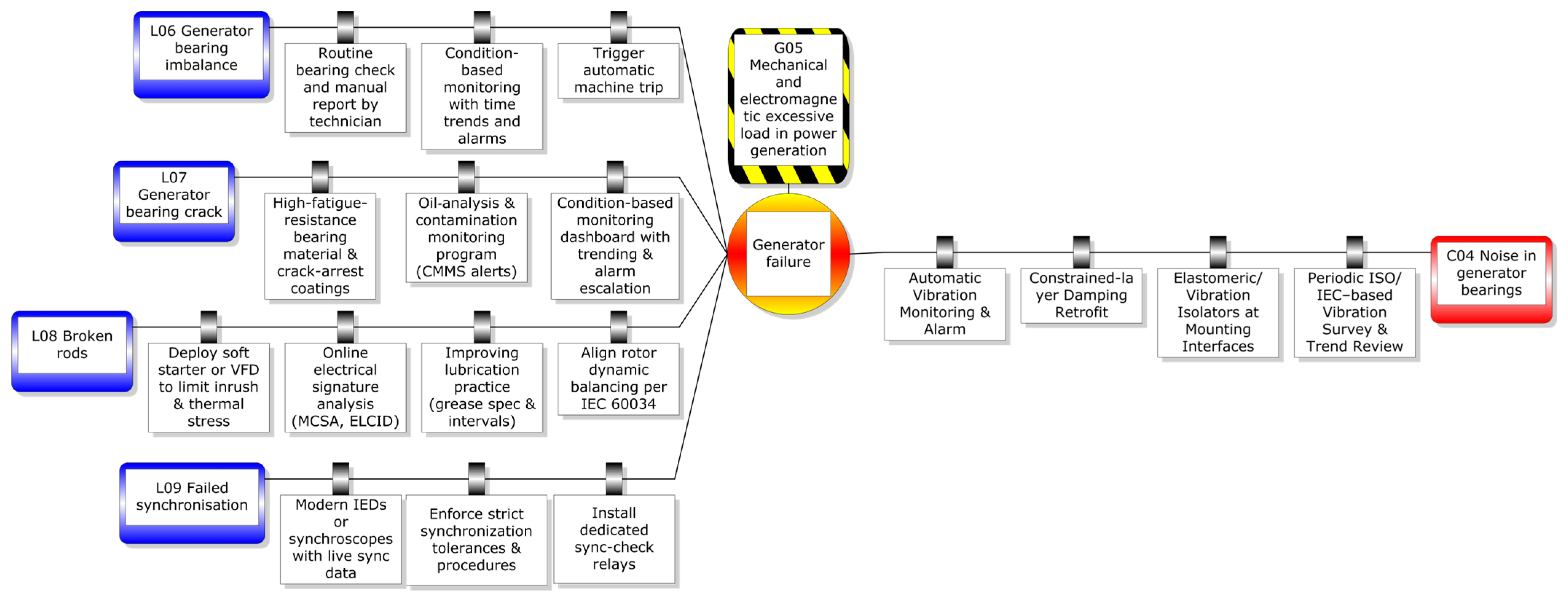
This paper is organised into six sections, including an introduction (Section 1) to promote a more precise understanding. Section 2 introduces the proposed framework architecture underlying the research. Section 3 concentrates on implementing the proposed framework in a case study of WT subsystems. Section 4 examines the results obtained from the BowTie framework computation. Section 5 discusses the outcomes produced by the proposed framework. Finally, Section 6 summarises the paper by reflecting on the significance and contributions of this study within the theoretical context.

2. Proposed BowTie Framework Architecture

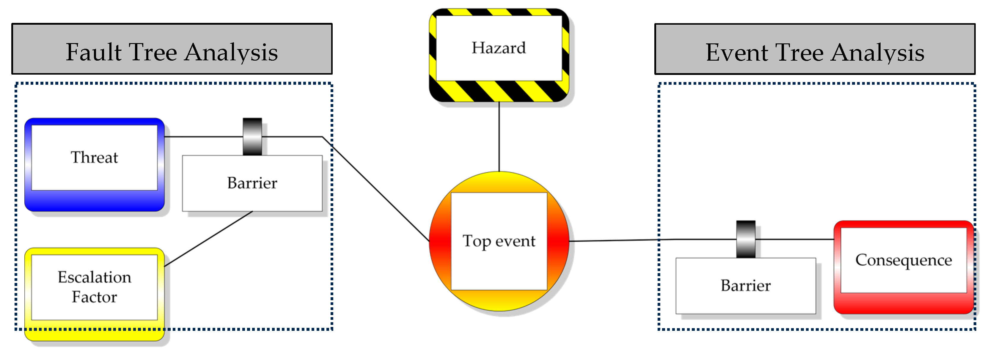
This section provides the conceptual and methodological foundation of the study. The unified BowTie framework adapts several core components from traditional BowTie analysis, such as hazard, TE, threat, consequence, barrier, and escalation factor. Standard BowTie analysis employs two main methods: FTA as the threat pathway and Event Tree Analysis (ETA) as the consequence pathway, as shown in Figure 1. Unlike traditional methods discussed in this paper, the BowTie model includes human and socio-technical factors, thus extending beyond purely mechanical systems. Its dual representation allows risks to be quantified and risk-informed in decision-making for safety and performance improvement.

Figure 1. Standard BowTie diagram.

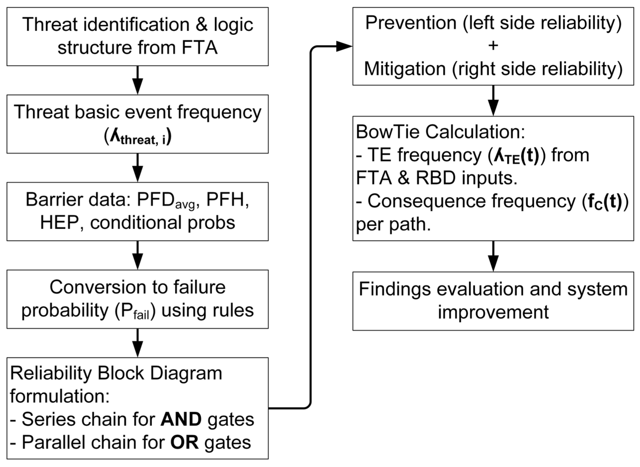
The proposed method enhances traditional BowTie by integrating RBD features, such as series, parallel, and k-out-of-n architectures, to arrange threat, barrier, and consequence positioning and sequencing, thereby offering a more flexible and scalable model. This integration follows a sequential workflow, as shown in Figure 2. First, FTA is initially developed to define threats and their causal structures, identifying logical combinations of basic events that lead to the TE. At this stage, it provides initial threat frequencies, ${\lambda }_{\mathrm{t}\mathrm{h}\mathrm{r}\mathrm{e}\mathrm{a}\mathrm{t},\mathrm{i}}$. Next, the barriers, such as PFD_avg, PFH, Human Error Probability (HEP) or conditional probability, P_conditional, are collected and converted into equivalent failure probability, P_fail, using standardised rules as presented in Table 2. This ensures consistent reliability representation and resolves unit mismatches between FTA probabilities and RBD reliability functions. Then, these barriers are organised in RBD, with AND gates represented as series chains and OR gates as parallel structures, preserving the logical relationships from FTA. These outputs are integrated into the BowTie framework, where the prevention side aims to avert threats, and the mitigation side manages the consequences if the TE occurs. This combination calculates the TE frequency, ${\lambda }_{\mathrm{T}\mathrm{E}}\left(t\right)$, and the associated consequence frequencies, ${\mathrm{f}}_C\left(t\right)$. The findings based on ${\lambda }_{\mathrm{T}\mathrm{E}}\left(\mathrm{t}\right)$ and ${\mathrm{f}}_C\left(t\right)$ metrics are evaluated to observe the model’s effectiveness.

Figure 2. The workflow of FTA, RBD, and the BowTie integration framework.

Table 2. Illustrative of the Barrier Catalogue and conversion rule.

Barrier Input Type	Barrier Expression Type	Unit Dimension	Conversion Rule
PFDavg	Low demand	Probability	${\lambda }_b$ = −ln(1 − PFDavg)/T ${\mathrm{P}}_{\mathrm{fail}} = 1 - {\mathrm{e}}^{-{\lambda }_{b}t}$
PFH	High demand/Continuous	Failure/hour	${\lambda }_b$ = PFH ${\mathrm{P}}_{\mathrm{fail}} = 1 - {\mathrm{e}}^{-{\lambda }_{b}t}$
HEP	Human reliability	Probability	Pfail = 1 − (1 − HEP)n
F(t)	Passive device reliability	Probability	Pfail = F(t)
Pconditional	Human + machine reliability	Probability	Pfail = Pconditional

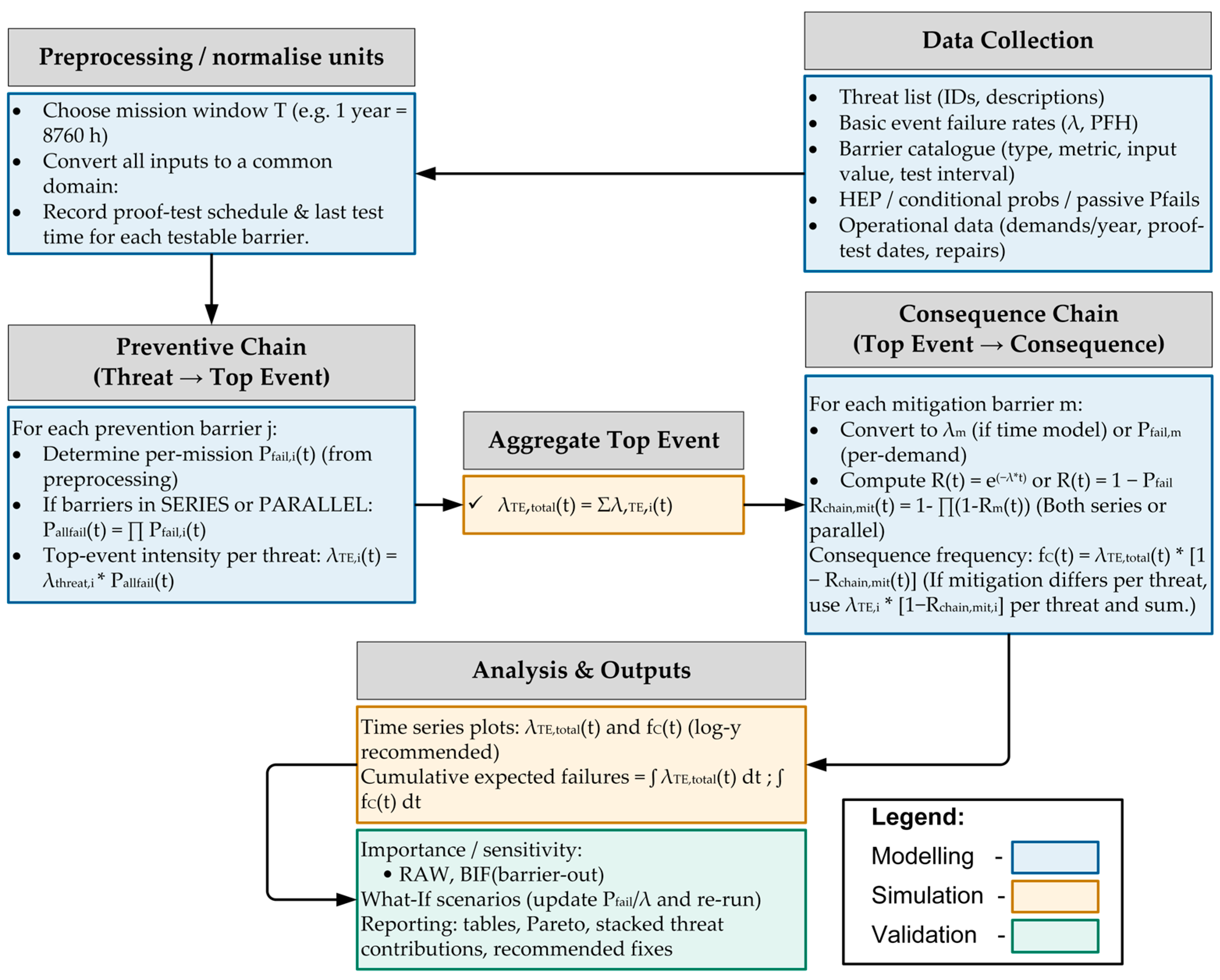
Figure 3 shows the detailed process flow in the proposed model to explain how it functions before exploring the following subsections.

Figure 3. The proposed unified Bowtie framework architecture.

2.1. Data Collection and Preprocessing

To advance the process, one should gather the data and preprocess it to achieve a consistent domain. The process starts with a list of threats derived from the basic event of FTA, which must be established beforehand, based on IEC 61025 [11]. The list should include the threat’s name, a unique identification code, and a description to facilitate easy tracking and identification. Each threat is then quantified with annual failure rates obtained from an established maintenance record, such as a Computerised Maintenance Management System (CMMS).

Another important tool in the proposed BowTie is the barrier’s information, also called the barrier catalogue. This catalogue includes details about preventive actions that stop threats from occurring. It contains the barrier name, barrier input type, expression type, unit dimension, role, input value, data sources and conversion rule, as illustrated in Table 2. Operational data such as annual demands, proof test dates, and repairs must be included in the catalogue.

Furthermore, it is important to note that before normalising input values into the same domain, the mission time, T, must be chosen, as each barrier may operate over different time intervals. Once T is selected, all input values of barriers are normalised into the same domain, such as converting failure rates into probabilities; this improves calculation accuracy. If the historical data are inconsistent across reporting years or incomplete, median values are used. Otherwise, if the data are missing, the values are supplemented by peer-reviewed literature or standard reliability databases. After data collection and normalisation are complete, the process moves on to the preventive chain side, as illustrated in Figure 3.

2.2. Preventive Pathway

The proposed framework’s preventive chain represents the left-hand side of the BowTie structure, where threats or basic events are systematically determined and controlled by proactive barriers before they escalate into the TE. Each barrier is selected from the barrier catalogue, which specifies its function, type and performance metric as demonstrated in Table 2. These quantitative metrics depend on barrier type, as outlined by the Centre for Chemical Process Safety (CCPS) [12]. Table 3 shows the mapping of barrier types and their corresponding quantitative metrics, along with descriptions.

Table 3. Barrier Types and Their Quantitative Metrics.

Barrier Type	Description	Quantitative Metrics
Behaviour	Human actions, operator compliance	HEP
Socio-technical	Organisational and systemic safeguards	Pconditional
Active hardware	Components that must act on demand	PFDavg
Continuous hardware	Barriers that operate continuously	PFH
Passive hardware	Inherent design features that require no intervention	F(t)

Each barrier is characterised by its attributes, as documented in the barrier catalogue. The proposed framework utilises RBD features by arranging barriers in series when there is a sequential dependence, or in parallel if there is redundancy, depending on the system architecture. For the preventive pathway, all equations are based on failure probability, similar to FTA. However, there is a slight difference when applying equations for series and parallel structures compared to the RBD and FTA theory models.

Within the BowTie model, regardless of whether the configuration is series or parallel, all barriers must fail for a TE to occur. As a result, both configurations have the same equations as follows:

$${\mathrm{P}}_{\text{all\_fail,pre,}i}(t) = {\prod }_{j\in {\mathcal{B}}_i}{\mathrm{P}}_{\mathrm{f}\mathrm{a}\mathrm{i}\mathrm{l},\mathrm{p}\mathrm{r}\mathrm{e},ij}\left(t\right)$$

(1)

where $j\in {\mathcal{B}}_i$ means that each preventive barrier j belongs to the set of preventive barriers, ${\mathcal{B}}_i$. P_fail,pre,ij(t) is the failure probability of each preventive barrier j within threat i by time, t, and P_{all_fail,pre,i}(t) is the prevention path failure probability for threat i when all barriers have failed by time t. The derivation of Equation (1) differs from conventional RBD and FTA methods. In FTA and RBD, a series system requires all components to work, so a single failure causes system failure. Conversely, parallel systems need only one component to operate; for instance, the system fails only if all components fail. In the BowTie approach, these logics do not apply because barriers act as sequential safeguards. For the TE to happen, every barrier in the chain must fail, regardless of how the barriers are arranged. Although the equation appears similar, the model still incorporates redundancy or parallelism to enhance reliability. From P_{all_fail,pre,i}(t), the TE frequency, ${\lambda }_{\mathrm{T}\mathrm{E}}\left(t\right)$, for each threat or basic event can be derived, as explained in Section 2.3 and Section 2.4.

Establishing barriers within the BowTie framework follows a few guiding principles, as recommended by CCPS [12]. First, the placement of barriers, whether triggered first or last, depends on the chronological sequence of their effect. This means preventive and mitigative barriers should be positioned logically based on their intended function. Second, active barriers, aside from those mentioned in Table 3, must incorporate elements of Detect-Decide-Action (DDA). Third, barriers’ properties should be independent, effective, and auditable. These principles are crucial for ensuring their proper functionality. Finally, to prevent common-mode failure, it is advisable to use more than one type of barrier on each pathway. Having multiple barrier types can compensate for the limitations of others and reduce the risk of simultaneous failure caused by a common cause.

2.3. Aggregate Top Event

At this stage, the goal is to compute the time-dependent aggregated TE frequency, ${\lambda }_{\mathrm{T}\mathrm{E}}\left(t\right)$, by summing the contributions of all initiating threats. Each threat’s contribution is calculated as the failure rate of the basic event multiplied by the probability that the entire preventive pathway fails, P_fail,pre,ij(t). The resulting ${\lambda }_{\mathrm{T}\mathrm{E}}\left(t\right)$, is then used to determine the frequencies of potential consequences, ${\mathrm{f}}_C\left(t\right)$. Table 4 represents a snapshot of the computation for each threat.

Table 4. Illustrative of each threat computation given barrier value and failure rate.

Threat	$\mathbf{Failure} \mathbf{Rate}$(λthreat,i)	Barrier	Input Value	Pfail,pre,ij(t)	Pall_fail,pre,i(t)	${\mathbf{\lambda }}_{\mathbf{T}\mathbf{E},\mathit{i}}$(t)
Threat i	Failure per hour	Behaviour	HEP	Conversion from input value to Pfail for each barrier	${\displaystyle \prod _{j=1}^{n_i}}{\mathrm{P}}_{\mathrm{f}\mathrm{a}\mathrm{i}\mathrm{l},\mathrm{p}\mathrm{r}\mathrm{e},ij\left(t\right)}$	${\lambda }_{\mathrm{t}\mathrm{h}\mathrm{r}\mathrm{e}\mathrm{a}\mathrm{t},i}$ ∗ Pall_fail,pre,i(t)
		Socio-technical	PConditional
		Active hardware	PFDavg
		Continuous hardware	PFH
		Passive hardware	F(t)

From Table 4, specific rules of the framework need to be adhered to obtain barrier failure probabilities from the input value. First, if the input value given is PFD_avg, it must be inverted numerically to determine an equivalent barrier failure rate, ${\lambda }_b$, by using the following:

$${\mathrm{PFD}}_{\mathrm{avg}} = 1-{\displaystyle \frac{1-{\mathrm{e}}^{-{\lambda }_{b}T}}{{\lambda }_{b}T}}$$

(2)

Equation (2) is solved numerically for ${\lambda }_b$ using an initial guess ${\lambda }_0$ ≈ 2∙PFD_avg/T. Then

$${\mathrm{R}}_{b,ij}\left(t\right)={\mathrm{e}}^{-{\lambda }_{b}t}$$

(3)

$${\mathrm{P}}_{\mathrm{fail},\mathrm{pre},ij}\left(t\right)=1-{\mathrm{R}}_{b,ij}=1-{\mathrm{e}}^{-{\lambda }_{b}t}$$

(4)

where ${\mathrm{R}}_{b,ij}$ is the reliability of each barrier j within threat i by time, t. Given that “t” is a mission time, T. Therefore, P_fail,pre,ij(T) = $1-{\mathrm{e}}^{-{\lambda }_{b}T}$.

Second, if the input value given is PFH (failures per hour), then PFH = ${\lambda }_b$. Therefore, Equation (4) can be used to determine P_fail,pre,ij(t). Otherwise, if the input value given is HEP (per-demand), then,

$${\mathrm{P}}_{\mathrm{fail},\mathrm{pre},ij}\left(T\right)=1-{\left(1-\mathrm{H}\mathrm{E}\mathrm{P}\right)}^n$$

(5)

In this case, n represents the number of demands during mission time, T, assuming the HEP remains constant. Lastly, if the input value is a conditional probability, P_conditional (socio-technical) or the probability of failure, F(t) (passive hardware), they are treated as per-mission P_fail,pre,ij(t) (constant),

$${\mathrm{P}}_{\mathrm{fail},\mathrm{pre},ij}\left(t\right)={\mathrm{P}}_{\mathrm{c}\mathrm{o}\mathrm{n}\mathrm{d}\mathrm{i}\mathrm{t}\mathrm{i}\mathrm{o}\mathrm{n}\mathrm{a}\mathrm{l}} \mathrm{O}\mathrm{R} \mathrm{F}\left(t\right)$$

(6)

It is worth noting that for time series plots, the study uses P_fail,pre,ij(t) as a vector over time, while HEP, P_conditional, and F(t) remain constant.

Next, in the proposed BowTie logic, a TE occurs only if all preventive barriers for threat i fail. When this happens, the individual P_fail,pre,ij(t) values for each preventive barrier in the threat are obtained, and Equation (1) is applied to multiply these P_fail,pre,ij(t) values together. This product equals P_{all_fail,pre,i} (t). The P_{all_fail,pre,i} (t) is then used in the following formula:

$${\lambda }_{\mathrm{T}\mathrm{E},i}\left(t\right)= {\lambda }_{\mathrm{t}\mathrm{h}\mathrm{r}\mathrm{e}\mathrm{a}\mathrm{t},i}\times {\mathrm{P}}_{\mathrm{a}\mathrm{l}\mathrm{l}\_\mathrm{f}\mathrm{a}\mathrm{i}\mathrm{l},\mathrm{p}\mathrm{r}\mathrm{e},i}\left(t\right)$$

(7)

${\lambda }_{\mathrm{T}\mathrm{E},i}\left(t\right)$ is the TE frequency of threat i, and ${\lambda }_{\mathrm{t}\mathrm{h}\mathrm{r}\mathrm{e}\mathrm{a}\mathrm{t},i}$ is the failure rate of threat i. Equation (7) calculates the individual threat contribution of TE intensity, ${\lambda }_{\mathrm{T}\mathrm{E},i}\left(t\right),$ by considering the probability of failure when all barriers are failed within that threat i. Each calculated ${\lambda }_{\mathrm{T}\mathrm{E},i}\left(t\right)$, based on the individual threat i is then aggregated together using the following formula:

$${\lambda }_{\mathrm{T}\mathrm{E}}\left(t\right)= {\sum }_i{\lambda }_{\mathrm{T}\mathrm{E},i}\left(t\right)$$

(8)

The ${\lambda }_{\mathrm{T}\mathrm{E}}\left(t\right)$ value is then used in Section 2.4 to determine the consequence frequency, ${\mathrm{f}}_C\left(t\right)$, in the mitigation pathway.

2.4. Mitigation Pathway

The mitigation pathway on the right side of the BowTie represents mitigative barriers that reduce the likelihood of a TE leading to a particular consequence. This study computes time-dependent mitigation reliabilities, R_mit,ck(t), combines them based on the system’s architecture, and determines how frequently consequences occur over time. The analysis process for the mitigation pathway closely resembles that of the prevention pathway, where the barrier input value from the barrier catalogue must be converted into P_fail,mit,ck(t), as shown in Table 4. From P_fail,mit,ck(t), the mitigation pathway is translated into reliability, R_mit,ck(t), reflecting the probability of the system successfully preventing the consequence. Combining these success probabilities in series or parallel yields the overall mitigation chain reliability R_chain,mit,c(t).

Apply the same conversion rules used for prevention. If the input value is PFD_avg, after solving Equation (2) to find ${\lambda }_b$, use the reliability formula as follows:

$${\mathrm{R}}_{\mathrm{mit},ck}\left(t\right) = {\mathrm{e}}^{-{\lambda }_{b}t},k\in {\mathcal{M}}_{\mathrm{c}}$$

(9)

where, $k\in {\mathcal{M}}_c$ means each mitigative barrier, k, belongs to the set of mitigative barriers, ${\mathcal{M}}_c$. R_mit,ck(t) is the mitigative barrier reliability, k, at each consequence, c. If the input value is PFH, it is considered equivalent to ${\lambda }_b$ (${\lambda }_b$ = PFH). Subsequently, Equation (9) is used to compute R_mit,ck(t). In case of HEP value for behavioural barrier, after solving Equation (5) and obtaining P_fail,mit,ck(t), then

$${\mathrm{R}}_{\mathrm{mit},ck}\left(t\right)=1-{\mathrm{P}}_{\mathrm{f}\mathrm{a}\mathrm{i}\mathrm{l},\mathrm{m}\mathrm{i}\mathrm{t},ck}\left(\mathrm{t}\right)$$

(10)

Equation (10) also applies to the input values of F(t) (passive barrier) and P_conditional (socio-technical barrier).

This study’s mitigation logic topology follows the defence-in-depth principle, where the consequences can be prevented if at least one mitigation measure succeeds. Conversely, the outcome only occurs if all mitigation layers fail. The defence-in-depth principle does not apply to FTA, ETA, and RBD, because, whether in series or parallel arrangements, both topologies require at least one mitigative barrier to prevent the effect. Therefore, to determine R_chain,mit,c(t), both cases use the same equation as follows:

$${\mathrm{R}}_{\mathrm{chain},\mathrm{mit},c}\left(t\right) = 1-{\prod }_{k\in {\mathcal{M}}_{\mathrm{c}}}\left(1-{\mathrm{R}}_{\mathrm{m}\mathrm{i}\mathrm{t},ck}\left(t\right)\right)$$

(11)

Given the aggregated TE frequency, ${\lambda }_{\mathrm{T}\mathrm{E}}\left(\mathrm{t}\right)$, obtained from Equation (8), the time-dependent consequence frequency, ${\mathrm{f}}_{C,c}\left(\mathrm{t}\right)$, is

$${\mathrm{f}}_{C,c}\left(t\right)={\lambda }_{\mathrm{T}\mathrm{E}}\left(t\right)\cdot \mathrm{Pr}\left\{\mathrm{m}\mathrm{i}\mathrm{t}\mathrm{i}\mathrm{g}\mathrm{a}\mathrm{t}\mathrm{i}\mathrm{o}\mathrm{n} \mathrm{c}\mathrm{h}\mathrm{a}\mathrm{i}\mathrm{n} \mathrm{f}\mathrm{a}\mathrm{i}\mathrm{l}\mathrm{s} \mathrm{a}\mathrm{t} t\right\}$$

(12)

Under defence-in-depth,

$${\mathrm{f}}_{C,c}\left(t\right)={\lambda }_{\mathrm{T}\mathrm{E}}\left(t\right)\times (1-{\mathrm{R}}_{\mathrm{c}\mathrm{h}\mathrm{a}\mathrm{i}\mathrm{n},\mathrm{m}\mathrm{i}\mathrm{t},c}\left(t\right))$$

(13)

If the BowTie framework includes several mitigation pathways resulting in multiple consequences, then Equation (13) can be reformulated as follows:

$${\mathrm{f}}_C\left(t\right)= {\sum }_{c=1}{\mathrm{f}}_{C,c}\left(t\right)$$

(14)

The computations above are then evaluated, and their outputs can serve as decision-support tools.

2.5. Barrier Parameterisation and Time-Dependent Mapping

In this study, time dependence is obtained directly from the exponential reliability model. The mission time is set to $T=8760$h (1 year), consistent with the typical annual operation and maintenance cycle of wind turbines and the reporting horizon of failure statistics in CMMS datasets. This choice ensures that the derived reliability metrics are directly aligned with industry practice and planning intervals. For any barrier characterised by PFD_avg (low demand) or PFH, the framework first maps the input to an equivalent constant failure rate ${\lambda }_b$, then computes the time-varying failure probability ${\mathrm{P}}_{\mathrm{f}\mathrm{a}\mathrm{i}\mathrm{l}}\left(\mathrm{t}\right)$ over the mission horizon [0 until 8760] $\left[0.8760\right]$ h with a 1 h step. When PFD_avg is specified over the mission time $T$ (here $T=8760$ h), ${\lambda }_b$ is obtained via Equation (2). When PFH is provided, the computation sets ${\lambda }_b=\mathrm{P}\mathrm{F}\mathrm{H}$. In both cases, once ${\lambda }_b$ is known, Equation (4) yields

$${\mathrm{P}}_{\mathrm{f}\mathrm{a}\mathrm{i}\mathrm{l}}\left(t\right)=1-{\mathrm{e}}^{-{\lambda }_{b}t},\mathrm{t}=0,1,2,\dots ,8760 \mathrm{h}.$$

These time series are then propagated through the BowTie logic to produce the top-event rate ${\lambda }_{\mathrm{T}\mathrm{E}}\left(t\right)$ and consequence frequency ${\mathrm{f}}_C\left(t\right)$, making the results explicitly time-dependent rather than single point values. This yields time-dependent results without imposing additional solver assumptions and relies only on the standard exponential form.

2.6. Evaluation, Decision Support and Framework Outputs

This section outlines the comparison framework and decision-support outputs used to assess BowTie scenarios. After calculating time-dependent reliability and availability metrics, as detailed in Section 2.2, Section 2.3 and Section 2.4, the study ranks barriers and threats using key measures such as BIF, and RAW. The framework also assesses design modifications like adding redundancy, reducing failure probabilities, and implementing process improvements through scenario comparisons. These evaluation results are summarised in tables and plots and integrated into a decision-making process that connects reliability improvements to practical interventions. This method facilitates transparent prioritisation of prevention and mitigation measures.

2.6.1. Importance Measures

Importance measures determine how each barrier influences overall system risk and aid in guiding design, testing, and investment decisions. This study uses two complementary measures, which are:

• Risk Achievement Worth (RAW) measures the increase in ${\lambda }_{\mathrm{T}\mathrm{E}}\left(t\right)$ if a particular barrier completely fails (${\mathrm{P}}_{\mathrm{f}\mathrm{a}\mathrm{i}\mathrm{l},ij}\left(t\right)$= 1). It assesses a barrier’s risk significance by comparing the baseline scenario to a scenario where the barrier is entirely failed. The RAW formula for barrier i is expressed as,

  $$\mathrm{RAW} ({\mathcal{B}}_i)={\displaystyle \frac{{\lambda }_{\mathrm{T}\mathrm{E}\left(\mathrm{n}\mathrm{e}\mathrm{w} \mathrm{t}\mathrm{o}\mathrm{t}\mathrm{a}\mathrm{l} \mathrm{w}\mathrm{h}\mathrm{e}\mathrm{n} {\mathcal{B}}_i \mathrm{r}\mathrm{e}\mathrm{m}\mathrm{o}\mathrm{v}\mathrm{e}\mathrm{d}\right)}}{{\lambda }_{\mathrm{T}\mathrm{E}\left(\mathrm{b}\mathrm{a}\mathrm{s}\mathrm{e}\mathrm{l}\mathrm{i}\mathrm{n}\mathrm{e} \mathrm{t}\mathrm{o}\mathrm{t}\mathrm{a}\mathrm{l}\right)}}}$$

  (15)

  ${\lambda }_{\mathrm{T}\mathrm{E}}\left(t\right)$ states that the TE frequency occurs with all barriers modelled as designed. On the other hand, ${\lambda }_{\mathrm{T}\mathrm{E}(\mathrm{n}\mathrm{e}\mathrm{w} \mathrm{t}\mathrm{o}\mathrm{t}\mathrm{a}\mathrm{l} \mathrm{w}\mathrm{h}\mathrm{e}\mathrm{n} {\mathcal{B}}_i \mathrm{r}\mathrm{e}\mathrm{m}\mathrm{o}\mathrm{v}\mathrm{e}\mathrm{d})}$ defines that the TE frequency occurs when barrier i is assumed always to fail (${\mathrm{P}}_{\mathrm{f}\mathrm{a}\mathrm{i}\mathrm{l},ij}\left(t\right)$ = 1). If RAW ≈ 1, this means barrier i has no significant influence on ${\lambda }_{\mathrm{T}\mathrm{E}}\left(t\right)$, and removing it barely changes them. Otherwise, if RAW ≥ 1, barrier i is highly risk significant and its failure leads to a substantial increase in ${\lambda }_{\mathrm{T}\mathrm{E}}\left(t\right)$. Therefore, RAW shows how much the risk affects the system if the barrier completely fails.

• The Barrier Importance Factor (BIF) identifies which barriers significantly reduce ${\lambda }_{\mathrm{T}\mathrm{E}}\left(t\right)$. It measures how much ${\lambda }_{\mathrm{T}\mathrm{E}}\left(t\right)$ could be lowered if these barriers were perfect. This concept offers a straightforward, quantitative method to prioritise improvements or actions for redundancy. The formula of BIF can be presented as follows:

  $$\mathrm{BIF} ({\mathcal{B}}_i)={\displaystyle \frac{{\mathrm{T}\mathrm{E}}_0-{\mathrm{T}\mathrm{E}}_i}{{\mathrm{T}\mathrm{E}}_0}}\times 100\%$$

  (16)

  TE₀ represents the baseline ${\lambda }_{\mathrm{T}\mathrm{E}}\left(t\right)$ with all barriers modelled as usual. Conversely, TE_i is the ${\lambda }_{\mathrm{T}\mathrm{E}}\left(t\right)$ if the barrier, ${\mathcal{B}}_i$, is considered perfect (${\mathrm{P}}_{\mathrm{f}\mathrm{a}\mathrm{i}\mathrm{l},ij}\left(t\right)$ = 0). A high BIF suggests that the barrier is crucial, and making it perfect could significantly lower the overall impact of ${\lambda }_{\mathrm{T}\mathrm{E}}\left(t\right)$.

All significant measure results are displayed and visualised using a bar chart, clearly illustrating the significance of the findings.

2.6.2. Sensitivity Analysis Workflow

This study adopts a structured, scenario-based sensitivity analysis workflow to evaluate potential design and operational improvements. It begins by establishing a baseline that represents the current system setup. From this baseline, it develops alternative scenarios reflecting proposed barrier upgrades. Each scenario is characterised by explicit modifications to barrier parameters, such as reducing oil system failure probability. Multiple parameter changes can also be combined into scenario sets, allowing the assessment of joint effects.

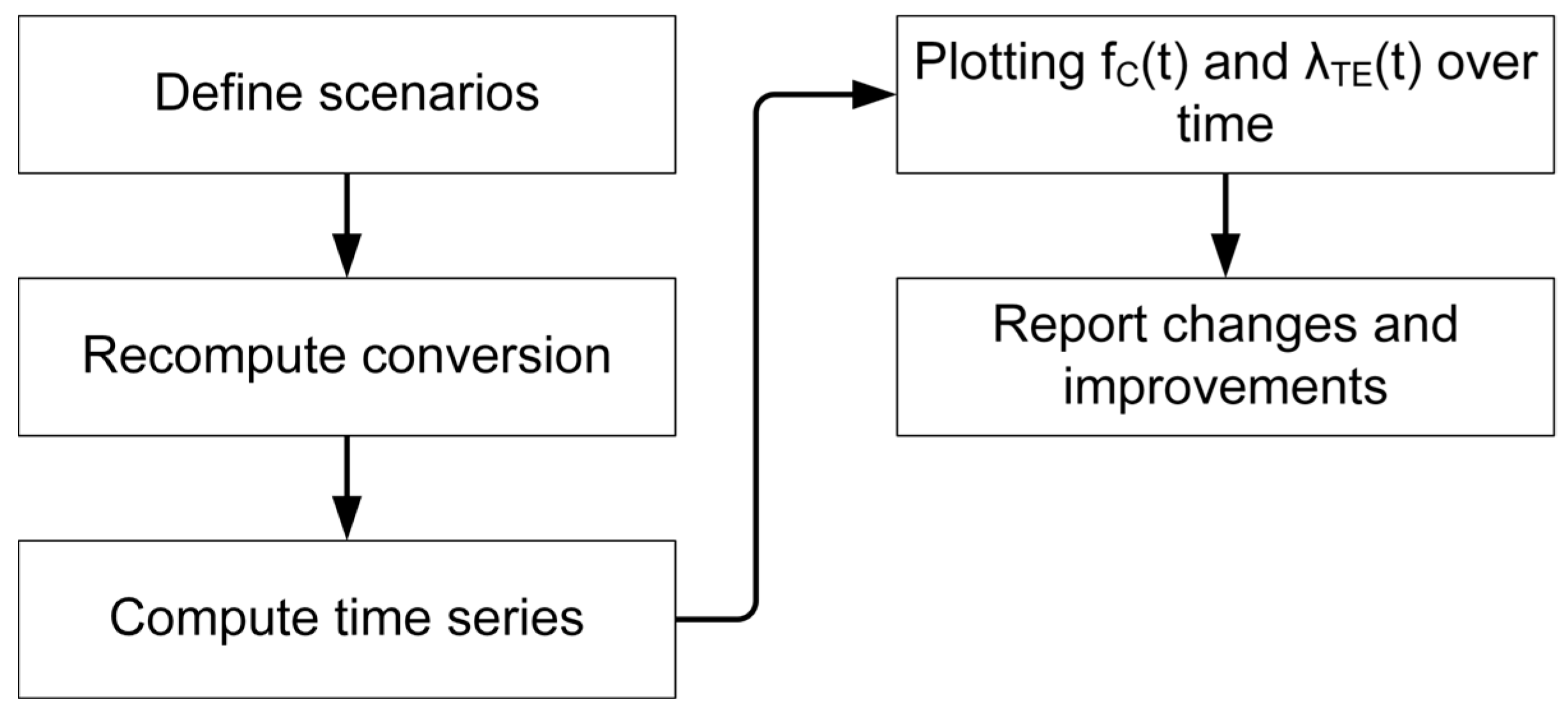
For each scenario, the reliability parameters are recomputed using the exact inversion, as described in Section 2.2, Section 2.3 and Section 2.4. This avoids potential hidden biases that may arise if baseline conversions are reused without modification. Finally, the comparison results are plotted over time, t, using ${\lambda }_{\mathrm{T}\mathrm{E}}\left(t\right)$ and ${\mathrm{f}}_C\left(t\right)$ as performance indicators to analyse the trend. The comparison framework is shown in Figure 4.

Figure 4. The comparison workflow for comparing baseline and alternative scenarios.

2.6.3. Model Efficiency

Model efficiency assesses computational and representational performance by comparing the BowTie aggregation to explicit ETA/FTA enumeration. This framework reports the minimal cut-set counts and sizes, and the total number of explicit event-tree sequences,

$${\mathrm{N}}_{\mathrm{ET}}={\sum }_{i=1}^{{\mathrm{N}}_{\mathrm{t}\mathrm{h}\mathrm{r}\mathrm{e}\mathrm{a}\mathrm{t}\mathrm{s}}}{2}^{n_{\mathrm{m}\mathrm{i}\mathrm{t},i}}$$

(17)

Each TE with the number of mitigation, n_mit, would branch per TE = $2^{n_{\mathrm{m}\mathrm{i}\mathrm{t},i}}$. The number of sequences the BowTie avoids representing explicitly is shown as follows:

$${\mathrm{N}}_{\mathrm{avoided}} = {\mathrm{N}}_{\mathrm{E}\mathrm{T}}-{\mathrm{N}}_{\mathrm{r}\mathrm{e}\mathrm{p}}$$

(18)

where N_rep indicates the number of sequences explicitly represented by the BowTie. Additionally, to validate the efficiency of the BowTie model, this framework compares the runtimes of calculating the consequence frequency, ${\mathrm{f}}_C\left(t\right)$, using the BowTie model versus explicit ETA enumeration. It also performs a numerical comparison of outcomes from both methods, ETA and BowTie, using the following formula:

$${\Delta }_f = \parallel {\mathrm{f}}_{C,\mathrm{b}\mathrm{o}\mathrm{w}}\left(T\right)-{\mathrm{f}}_{C,\mathrm{E}\mathrm{T}}\left(T\right){\parallel }_{\mathrm{\infty }}$$

(19)

This value is then reported to assess whether it lies within tolerance.

3. Case Study

This section demonstrates how the proposed BowTie-reliability framework can be applied through a real case study. The study referenced here is conducted initially by Ozturk [12], who examines WT failures using reliability methods and Machine Learning (ML). Ozturk focused solely on identifying criticality, modelling reliability, and predicting WT failure. However, this paper sees potential to expand the scope further, motivating the application of the proposed BowTie framework using Ozturk’s foundational information. Although their study addresses many reliability issues related to WT, it does not aim to reduce failure risks, prevent the TE, or mitigate failure consequences—areas prioritised here. As a result, this work develops two common reliability models, the FTA and RBDs, based on Ozturk’s data and additional insights from related studies. From this foundation, the BowTie model is constructed, assessed, and discussed.

3.1. Background of the Case Study

Wind energy is widely regarded as a leading renewable resource among alternative energy sources. Its environmentally friendly and sustainable qualities have driven rapid growth in its deployment. As the failure rate of WT increases significantly, the focus has shifted toward enhancing their reliability and availability to ensure continuous power generation. The study led by Ozturk, part of the Scientific Measurement and Evaluation Programme (WMEP) in Germany, is a key component of a government effort to analyse onshore WTs from 1989 to 2006. It compiled 64,000 maintenance and repair reports from 1500 turbines, representing over 15,000 years of operational data. Ozturk’s findings provide valuable insights into WT reliability, aiding the development and validation of a reliability modelling framework.

This study focuses on the generator as a key subcomponent of the WT system, selected based on its criticality in prior research. Both Ozturk [13] and Parnon et al. [14] identify the generators as the highest-ranked subsystem in their criticality analyses, though derived from different frameworks. This finding is also supported by Pulikollu et al. [15], who consistently identify generators as the most vulnerable and costly assets, with failures such as imbalance, cracking, or lubrication deficiencies leading to sudden breakdowns, extended downtime, and high replacement costs. While the generator’s annual failure rate falls within the range of 1% to 4%, its downtime may lead to significant production losses and unplanned repair costs, estimated at around $100,000 to $225,000 [15]. Owing to this criticality, the generator is selected for developing the FTA and demonstrating the proposed framework. The following section provides further details on the development of both approaches.

3.2. Development of Reliability Modelling

This section illustrates the development of the FTA and RBDs based on a study conducted by Ozturk [13] and other studies [16,17,18]. It starts with comparing several established FTA diagrams created by Novaković et al. [16], Márquez et al. [17], and Kang et al. [18]. To produce an FTA based on these established studies, a screening criterion is specified as follows:

• Include if:
  • Mentioned in ≥2 literature sources OR
  • Found in the dataset OR
  • Has a significant impact

As stated in Section 3.1, this study focuses on the generator as a subcomponent of the WT that requires evaluation. Consequently, Figure 5 illustrates an FTA diagram of the WT generator, developed based on the referenced studies [16,17,18] and screening criteria. Table 5, furthermore, showcases the list of TEs, intermediate events, and basic events with sources of references.

Figure 5. FTA diagram of WT generator for the case study.

Table 5. Logic gates and principal events of the WT generator.

Logic Gates	Codes	Basic Events	Codes
Generator failure	G5	Bearing Imbalance	L6
Bearing Failure	G9	Bearing Crack	L7
Rotor and Stator Failure	G10	Broken rods	L8
		Failed Synchronisation	L9

The RBD model, in Figure 6, is derived from the FTA diagram in Figure 5, based on studies by Ozturk [13], Einarsson et al. [19], and Linsday et al. [20]. Afterwards, the minimal cut set equation is formulated to construct the BowTie model.

Figure 6. RBD model of WT Generator.

Based on the FTA and RBDs, a minimal cut set can be formulated to determine the smallest set of subcomponent failures needed to cause the entire system to fail. The logic operator in Figure 5 consists solely of OR gates, which correspond to the arithmetic “+” sign in accordance with IEC 61025 [11]. Using this convention, the minimal cut set formula can be derived as follows:

$$Fail state=G_5$$

(20)

$$G_5=G_9+G_{10}$$

(21)

$$G_9=L_6+L_7$$

(22)

$$G_{10}=L_8+L_9$$

(23)

Derivation involving Equations (20)–(23) generates the final minimal cut set equation:

$$Fail state=L_6+ L_7+L_8+L_9= \left\{L_6, L_7,L_8,L_9\right\}$$

(24)

L₆, L₇, L₈, and L₉ constitute the primary first-order minimal cut sets that need to be emphasised in the BowTie model.

3.3. Development of BowTie Model

The BowTie model, clarified in Section 2 with an illustrative diagram in Figure 1 consists of several components, including the hazard, TE, the preventive pathway (left), the mitigation pathway (right), and the associated barriers. This subsection describes how the BowTie model is developed using a case study centred on the minimal cut set identified in Section 3.2.

Section 3.2 of this study reveals that L₆, L₇, L₈, and L₉ are the fundamental events of the developed FTA model in Figure 5. As first-order events, their states are highly susceptible to failure and need focused improvement. To convert information from FTA and RBD into the BowTie model, the minimal cut set is directly identified as threats. The consequences or effects of the TE follow the taxonomy of Ozturk [13]. Barriers, preventive and mitigative, are selected from the literature and industry practice to address each threat and consequence. The full BowTie diagram is presented in Figure 7.

Figure 7. The proposed BowTie model for the WT generator.

To ensure transparency and reproducibility, this study provides supporting materials alongside the BowTie model, including the assumption table listing modelling assumptions and units and quantitative data, such as failure rate and probability. The calculation methods have been presented in Section 2, from Equations (1)–(19). This information is summarised in tabular form, where Table 6 exhibits the modelling assumptions and metrics, Table 7 presents BowTie core elements, while Table 8, Table 9, Table 10, Table 11 and Table 12 detail the preventive and mitigative barriers associated with specific threats and consequences, supported by quantitative evidence from prior studies. The assumptions in Table 6 are adopted for demonstration purposes to keep the case study tractable; they are not rigid requirements of the framework and can be relaxed or adjusted depending on the application context.

Table 6. The modelling assumptions and metrics.

Item	Assumption	Notes
Time basis	Steady-state reliability with constant failure rate.	h
Barrier independence	Barriers are assumed to be independent unless noted; common cause failure is negligible.	−
Threat failure rate	Taken directly from the literature survey.	Failures/h
Mission time, Tmission	Use 8760 h = 1 year.	h
PFH	Continuous failure rate measure.	Failures/h
PFDavg	Demand frequency is assumed annually.	Probability/demand
Pfail	Point probability of the component failure.	dimensionless
Pconditional	Conditional probability that monitoring fails to detect the threat.	dimensionless
HEP	Derived from human reliability analysis (THERP/SPAR-H)	Probability/event
Maintainability	The repair rate is assumed to be negligible; The renewal function is used (part replaced “as good as new”)	−

Table 7. The proposed BowTie core elements.

Element Type	Element Name	Failure Rate (Failure/h)	Sources
Hazard	Mechanical and electromagnetic excessive load in power generation	−	[13]
TE	Generator failure	−	[13]
Threat (L6)	Generator bearing imbalance	5.85 × 10−6	[18]
Threat (L7)	Generator bearing crack	1.17 × 10−6	[18]
Threat (L8)	Broken rods	2.10 × 10−7	[18]
Threat (L9)	Failed synchronisation	3.61 × 10−6	[18]

Table 8. Preventive barriers by threat (L₆).

Barrier	Category	Type	Input Value	Sources
Routine bearing check and manual report	Behavioural	HEP	1.10 × 10−1	[21]
CBM with time trends and alarms	Socio-technical	Pconditional	3.00 × 10−2	[21,22]
Trigger automatic machine trip	Active hardware	PFDavg	6.20 × 10−6	[23]

Table 9. Preventive barriers by threat (L₇).

Barrier	Category	Type	Input Value	Sources
High-fatigue-resistance bearing material and crack-arrest coatings	Passive hardware	Pfail	2.40 × 10−2	[24,25]
Oil-analysis and contamination monitoring program (CMMS alerts)	Socio-technical	Pconditional	7.20 × 10−1	[26]
CBM dashboard with trending and alarm escalation	Socio-technical	Pconditional	1.00 × 10−1	[27]

Table 10. Preventive barriers by threat (L₈).

Barrier	Category	Type	Input Value	Sources
Deploy soft starter or VFD (Variable Frequency Drive) to limit inrush and thermal stress	Continuous hardware	PFH	3.50 × 10−6	[28]
Online electrical signature analysis	Active hardware	PFDavg	3.00 × 10−2/demand	[29]
Improving lubrication practice (grease spec and intervals)	Behavioural	HEP	3.00 × 10−3	[30]
Align rotor dynamic balancing per IEC 60034	Behavioural	HEP	1.00 × 10−3	[30]

Table 11. Preventive barriers by threat (L₉).

Barrier	Category	Type	Input Value	Sources
Modern IEDs (Intelligent Electronic Device) or synchroscopes with live sync data	Socio-technical	Pconditional	1.70 × 10−2	[31]
Enforce strict synchronisation tolerances and procedures	Behavioural	HEP	3.00 × 10−2	[21,30]
Install dedicated sync-check relays	Active hardware	PFDavg	1.80 × 10−6/demand	[32]

Table 12. Mitigative barriers by Consequence (C₀₄).

Barrier	Category	Type	Input Value	Sources
Automatic Vibration Monitoring and Alarm	Active hardware	PFDavg	1.20 × 10−3	[33]
Constrained-layer Damping Retrofit	Passive hardware	Pfail	2.00 × 10−2	[34]
Elastomeric/Vibration Isolators at Mounting Interfaces	Passive hardware	Pfail	3.00 × 10−2	[35]
Periodic ISO/IEC–based Vibration Survey and Trend Review	Behavioural	HEP	1.00 × 10−2	[30]

Finally, the results and discussion sections include model validation. The validity of key modelling assumptions, as mentioned in Table 6 is implicitly tested through scenario-based sensitivity analysis in Section 2.6.2 and Section 3.4. By systematically varying barrier parameters, this analysis provides analytical insights into how deviations from baseline assumptions influence ${\lambda }_{\mathrm{T}\mathrm{E}}\left(\mathrm{t}\right)$ and ${\mathrm{f}}_C\left(\mathrm{t}\right)$.

3.4. Sensitivity Analysis

As outlined in Section 2.6.2, a sensitivity analysis is conducted to evaluate the robustness of the model by systematically varying key barrier parameters. Each manipulation represents a distinct scenario to observe the resulting trends in both ${\lambda }_{\mathrm{T}\mathrm{E}}\left(\mathrm{t}\right)$ and ${\mathrm{f}}_C\left(\mathrm{t}\right)$. In this case study, there are four scenarios, with one baseline for comparison purposes. Table 13 summarises these scenarios, where each represents modifications in barriers such as redundancy, reduction, and frequent proof-test frequency, as well as combined improvements across multiple barriers.

Table 13. Sensitivity analysis scenarios.

Scenario	Barrier Modified	Parameter Adjustment
Baseline	None	Reference value
Oil analysis improved	Oil lab protection	Pfail reduced from 0.72 to 0.20
Redundant dashboard	Dashboard	Addition of a 2nd independent dashboard
Faster auto-alarm proof-test	Auto-alarm	PFDavg halved Oil analysis and dashboard applied together
Combined (Oil + Dashboard)	Oil lab protection, dashboard

Each scenario is analysed and evaluated using the outlined workflow in Figure 4. The findings are then explained in Section 4.4.

4. Results

This section highlights the analysis results from the BowTie model applied to the WT case study. The outcomes emphasise WT’s reliability performance and the strategies for preventing and mitigating major failures. Findings are organised according to the research question outlined in Section 1, focusing on four key measurable aspects: risk contribution ranking, quantitative assessment of barrier adequacy, reliability improvements through scenario-based sensitivity analysis, and overall model efficiency.

Using Equation (1) through (19) with the provided information from Table 6, Table 7, Table 8, Table 9, Table 10, Table 11 and Table 12, the results are shown in Table 14, which addresses four measurable aspects of outcomes. The inversion of PFD_avg values into ${\lambda }_b$ is implemented using the built-in fzero function in MATLAB R2025a Update 1 (Version 25.1.0.2973910). Initial guesses for ${\lambda }_b$ are taken from ${\lambda }_0$ ≈ 2∙PFD_avg/T, where T = 8760 h represents one year of operation. Convergence is accepted when the absolute residual of the inversion equation, $\mathsf{ϵ}=1-{\displaystyle \frac{1-{\mathrm{e}}^{-bT}}{{\lambda }_{b}T}}-{\mathrm{P}\mathrm{F}\mathrm{D}}_{\mathrm{a}\mathrm{v}\mathrm{g}}^{\mathrm{T}\mathrm{a}\mathrm{r}\mathrm{g}\mathrm{e}\mathrm{t}}$, is less than ${1 \times 10}^{-10}$, where all results are well within tolerance between ${10}^{-12}$ and ${10}^{-14}$, as presented in Table 15. However, if the residual is unable to achieve within the specified tolerance, the ${\lambda }_b$ value is taken from the approximated equation, 2∙PFD_avg/T.

Table 14. Summary of BowTie outcomes.

Preventive Barrier	${\mathbf{P}}_{\mathbf{a}\mathbf{l}\mathbf{l}\_\mathbf{f}\mathbf{a}\mathbf{i}\mathbf{l},\mathbf{p}\mathbf{r}\mathbf{e},\mathit{i}}$(t)	${\mathbf{\lambda }}_{\mathbf{T}\mathbf{E}}$(t) Contributions (Failures/h)
Threat L06:	2.046 × 10−7	1.197 × 10−12
Routine bearing check and manual report
Condition-based monitoring with time trends and alarms
Trigger automatic machine trip
Threat L07:	1.728 × 10−3	2.022 × 10−9
High-fatigue-resistance bearing material and crack-arrest coatings
Oil-analysis and contamination monitoring program (CMMS alerts)
Condition-based monitoring dashboard with trending and alarm escalation
Threat L08:	5.380 × 10−9	1.130 × 10−15
Deploy soft starter or VFD to limit inrush and thermal stress.
Online electrical signature analysis.
Improving lubrication practice (grease spec and intervals).
Align rotor dynamic balancing per IEC 60034.
Threat L09:	1.836 × 10−9	6.628 × 10−15
Modern IEDs or synchroscopes with live sync data.
Enforce strict synchronisation tolerances and procedures.
Install dedicated sync-check relays.
Total λTE (sum of contributions)	2.023 × 10−9 failures/h
Mitigative Barrier	${\mathbf{P}}_{\mathbf{a}\mathbf{l}\mathbf{l}\_\mathbf{f}\mathbf{a}\mathbf{i}\mathbf{l},\mathbf{m}\mathbf{i}\mathbf{t},\mathit{c}}$(t)	${\mathbf{f}}_{\mathit{C}}$ (t) Contributions (Failures/h)
Consequence C04:	1.439 × 10−8	2.912 × 10−17
Automatic Vibration Monitoring and Alarm
Constrained-layer Damping Retrofit
Elastomeric/Vibration Isolators at Mounting Interfaces
Periodic ISO/IEC–based Vibration Survey and Trend Review
$\mathrm{Total} {\mathrm{f}}_C\left(t\right)$$(\mathrm{Product} \mathrm{of} \mathrm{total} {\lambda }_{\mathrm{T}\mathrm{E}}(\mathrm{t})$ and total Pall_fail,mit(t))		2.912 × 10−17 failures/h

Table 15. Validation of PFD_avg-to-${\lambda }_b$ inversion for selected barriers (mission time T = 8760 h).

Barrier (Type)	Target PFDavg	${\mathbf{\lambda }}_{\mathit{b}}$	Residual
L06 (PFDavg)	3.100 × 10−5	7.078 × 10−9	−5.151 × 10−14
L08 (PFDavg)	3.000 × 10−2	6.990 × 10−6	−4.038 × 10−14
L09 (PFDavg)	1.800 × 10−6	4.110 × 10−10	2.077 × 10−12
Mitigation (PFDavg)	1.200 × 10−3	2.742 × 10−7	−1.823 × 10−14

4.1. Risk Contribution Ranking

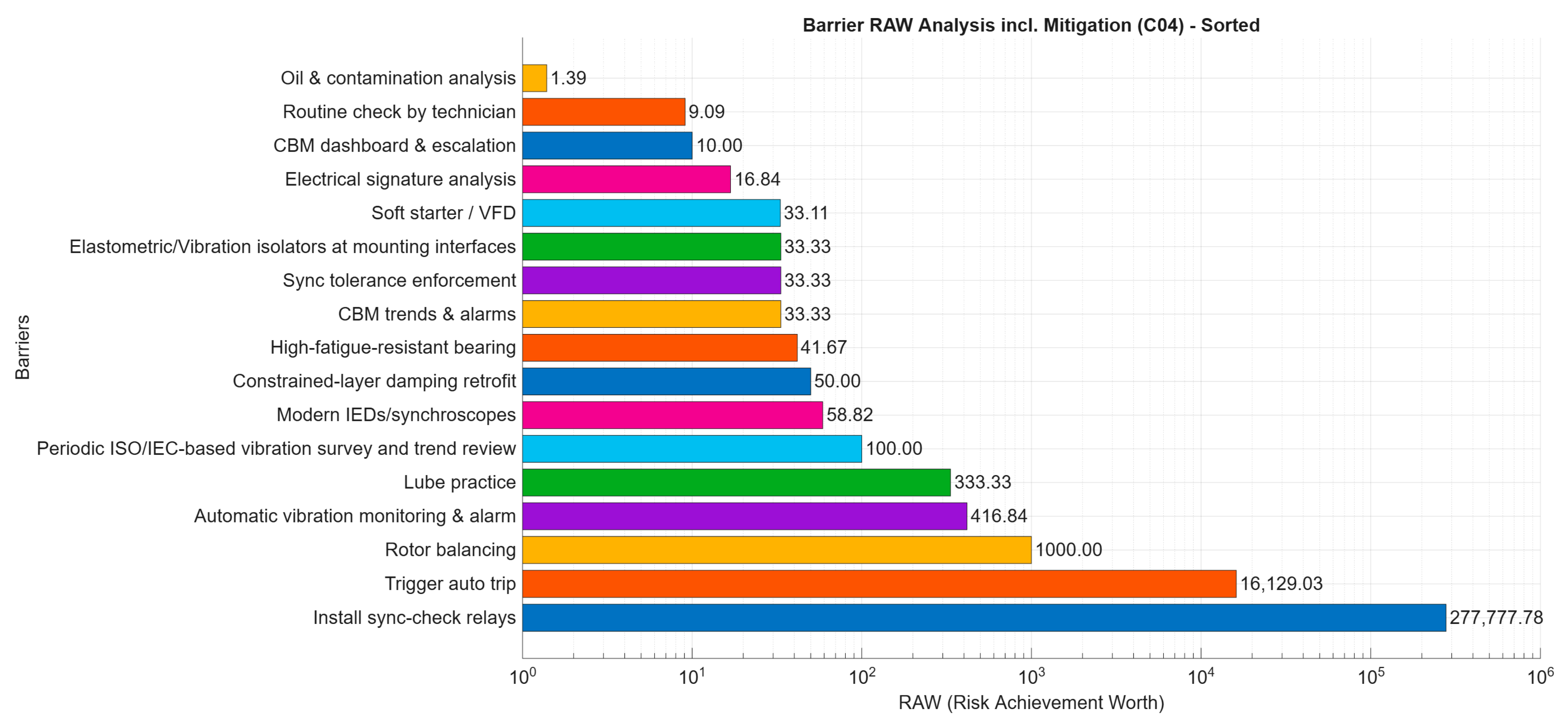
RAW analysis, as described in Section 2.6.1, assesses barriers’ contribution to ${\lambda }_{\mathrm{T}\mathrm{E}}\left(t\right)$ assuming they fail completely. Figure 8 indicates that most barriers have relatively low RAW values, such as the CBM dashboard, routine checks, and oil analysis. This suggests that their absence would only slightly raise ${\lambda }_{\mathrm{T}\mathrm{E}}\left(t\right)$. However, a few barriers show very high RAW values, notably the sync-check relays and trigger auto trip, which exceed 10⁴. Additionally, rotor balancing, lube practice, and modern IED are also highly critical. These barriers act as vital single points of defence, with their effectiveness significantly controlling the likelihood of avoiding a hazardous outcome.

Figure 8. Barrier RAW analysis, including mitigation outcomes.

The pattern also demonstrates the defence-in-depth approach of the BowTie model. Barriers relying solely on human action, like lubrication practices, or static hardware, such as a soft starter, provide additional protection. However, active barriers, such as auto-trip triggers or check relays, play a more significant role in the RAW distribution. This suggests that while barriers not aligned with DDA elements can help mitigate hazards, those fulfilling DDA criteria are primarily responsible for protecting the system.

From a decision perspective, RAW analysis indicates that prioritising investment in maintaining and testing high-RAW barriers is crucial, since their failure could lead to exponential increases in system risk. Conversely, for barriers with lower RAW values, the model suggests they still contribute to system resilience but may need optimisation or streamlining, ensuring safety remains unaffected.

4.2. Barrier Importance Factor

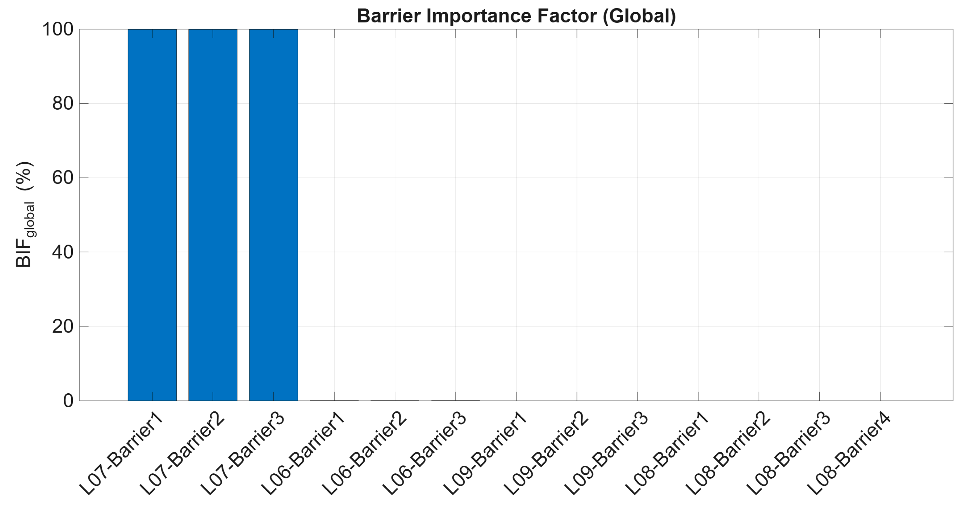
The BIF measures how much each preventive barrier helps prevent ${\lambda }_{\mathrm{T}\mathrm{E}}\left(t\right)$. A higher BIF shows that improving these barriers can significantly reduce ${\lambda }_{\mathrm{T}\mathrm{E}}\left(t\right)$. Figure 9 displays the BIF results from the BowTie model.

Figure 9. Barrier Importance Factor with respect to ${\lambda }_{\mathrm{T}\mathrm{E}}\left(t\right)$.

Figure 9 clearly shows that all three preventive barriers under threat L₀₇ collectively contribute 100% to the ${\lambda }_{\mathrm{T}\mathrm{E}}\left(t\right)$. This implies that the effectiveness of preventing the TE from happening is dependent on maintaining these barriers at their proper functioning level. Furthermore, these results also highlight that L₀₇ is fully controlled by its associated barriers, meaning any failure or removal of these barriers would directly lead to an increase in ${\lambda }_{\mathrm{T}\mathrm{E}}\left(t\right)$. Unlike other threats, where barrier contributions barely emerge and are distributed unevenly, L₀₇ requires rigorous monitoring and maintenance.

4.3. Barrier Quantitative Assessment over Time

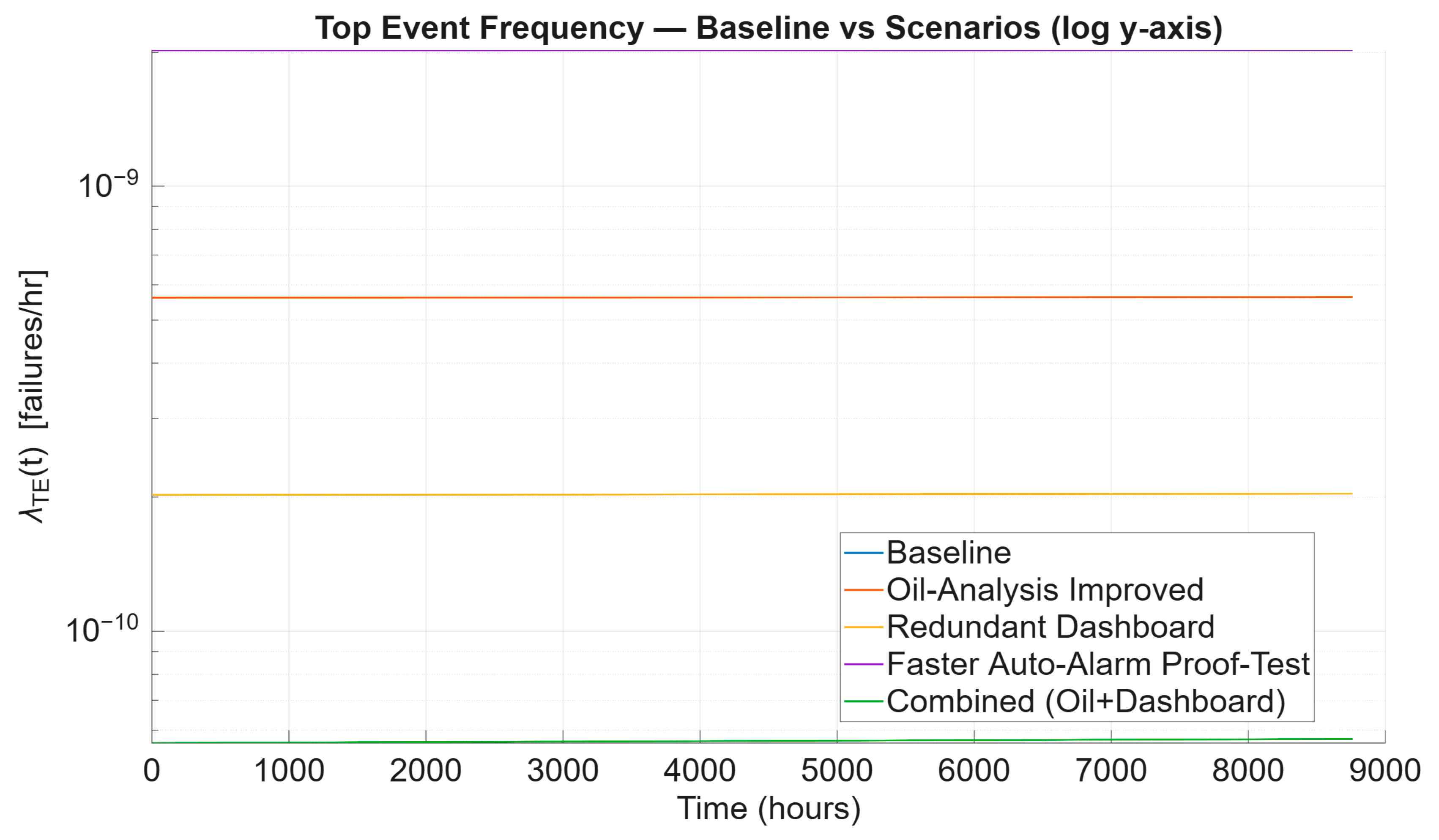
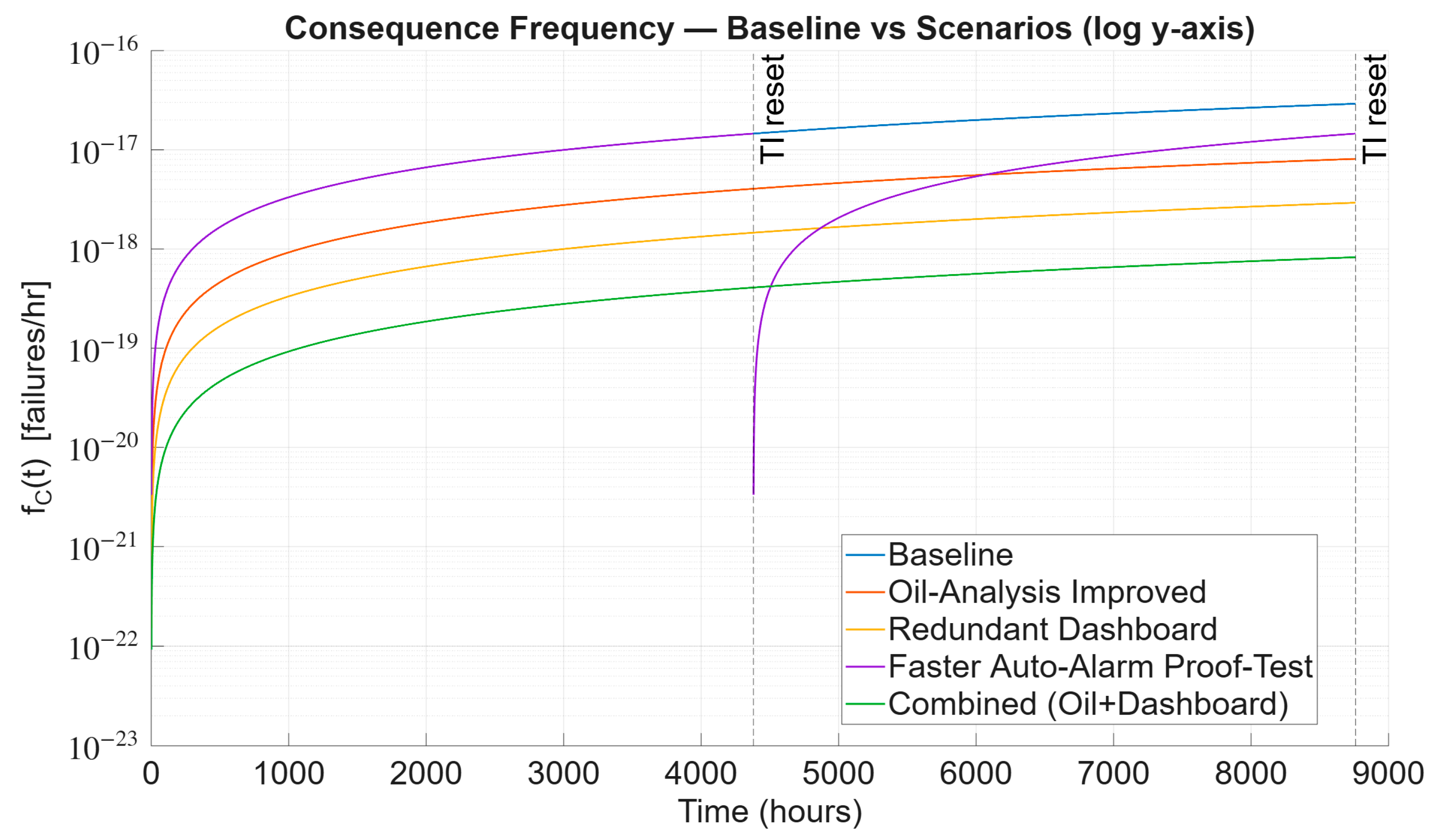
This section shows the trends of ${\lambda }_{\mathrm{T}\mathrm{E}}\left(t\right)$ and ${\mathrm{f}}_C\left(t\right)$ over mission time, T. The goal is to observe how barrier systems behave along with their threats and consequences as time progresses. Figure 10 and Figure 11 display the ${\lambda }_{\mathrm{T}\mathrm{E}}\left(t\right)$ and ${\mathrm{f}}_C\left(t\right)$ over a year, or 8760 h. As explained in Section 2.5, in all cases, barriers parameterised by PFD_avg (over $T=8760$ h) or PFH are mapped to an equivalent constant rate ${\lambda }_b$, and their time-varying failure probability is computed using Equation (4). This gradual increase in ${\mathrm{P}}_{\mathrm{f}\mathrm{a}\mathrm{i}\mathrm{l}}\left(t\right)$ over $t$ explains the near-linear growth of ${\lambda }_{\mathrm{T}\mathrm{E}}\left(t\right)$ under constant ${\lambda }_{\mathrm{t}\mathrm{h}\mathrm{r}\mathrm{e}\mathrm{a}\mathrm{t}}$ and ${\lambda }_b$ from approximately 2.02 × 10⁻⁹ to 2.023 × 10⁻⁹ failures per hour during the mission, as shown in Figure 10. Although the increase is monotonic, the change remains minimal, indicating that barrier degradation is slow and the preventive configuration sustains a consistently low top-event rate across the operating horizon.

Figure 10. The ${\lambda }_{\mathrm{T}\mathrm{E}}\left(t\right)$ pattern over mission time, T.

Figure 11. The ${\mathrm{f}}_{\mathrm{C}}\left(t\right)$ pattern over mission time, T.

Figure 11 illustrates how ${\mathrm{f}}_C\left(t\right)$ evolves over time, showing a rapid increase from 0 to 2000 h during the early mission phase. After this period, it gradually stabilises around 10⁻¹⁸ failures per hour. This effectively prevents the escalation of TE into serious consequences. The data suggest that, within a defence-in-depth framework, the occurrence of severe outcomes remains very low.

The combined reliability analysis shows that although ${\lambda }_{\mathrm{T}\mathrm{E}}\left(t\right)$ continues to rise over time because of barrier wear-out, the mitigation measures keep the impact of TE very low (≤10⁻¹⁷/h). This indicates the long-term effectiveness of the defence-in-depth strategy.

4.4. Scenario-Based Sensitivity Analysis Outcomes

Section 4.4 assesses the impact of barrier modifications on system reliability using a series of what-if scenarios outlined in Section 3.4. The findings are presented in tabular format in Table 16 and graphically in Figure 12 and Figure 13 to enable a quantitative and visual evaluation of barrier performance.

Table 16. The outcomes of scenario-based sensitivity analysis outcomes.

Scenario	${\mathbf{\lambda }}_{\mathbf{T}\mathbf{E}}\left(\mathbf{t}\right)$	${\mathbf{f}}_{\mathit{C}}\left(\mathbf{t}\right)$	% Reduction vs. Baseline	Notes
Baseline	2.023 × 10−09	2.912 × 10−17	−	Reference inputs
Oil -Analysis Improved	5.628 × 10−10	8.101 × 10−18	72.18	Oil Pfail 0.72 → 0.20
Redundant Dashboard	2.034 × 10−10	2.034 × 10−18	89.95	Dashboard Pfail 0.10 → 0.01
Faster Auto-Alarm Proof-Test	2.022 × 10−09	2.911 × 10−17	0.03	PFDavg halved
Combined (Oil + Dashboard)	5.736 × 10−11	8.257 × 10−19	97.16	Both improvements applied

Figure 12. The baseline vs. scenarios of ${\lambda }_{\mathrm{T}\mathrm{E}}\left(\mathrm{t}\right)$.

Figure 13. The baseline vs. scenarios of ${\mathrm{f}}_{\mathrm{C}}\left(\mathrm{t}\right)$.

Table 16 shows that the baseline case results for both ${\lambda }_{\mathrm{T}\mathrm{E}}\left(t\right)$ and ${\mathrm{f}}_C\left(t\right)$ are 2.023 × 10⁻⁹ failures per hour and 2.912 × 10⁻¹⁷ failures per hour, which serve as the reference point for comparison. Both tabular and graphical results display this as the highest frequency, emphasising the system’s vulnerability under the current barrier effectiveness.

In the initial alternate scenario, the failure probability of the oil analysis barrier decreases from 0.72 to 0.20. As a result, ${\mathrm{f}}_C\left(t\right)$ drops sharply to 8.101 × 10⁻¹⁸ failures per hour, marking a 72.18% reduction. This notable decline is clearly shown in Figure 12 and Figure 13, where the curve for this scenario diverges significantly from the original baseline.

Focusing on the redundant dashboard scenario, it significantly benefits by reducing 89.95% of ${\mathrm{f}}_C\left(t\right)$, equating to 2.034 × 10⁻¹⁸ failures per hour. Figure 12 and Figure 13 show these findings, with the dashboard curve positioned well below the baseline and oil-analysis curves, highlighting the substantial impact of redundancy in operator interface barriers.

In contrast, cutting the proof-test interval of the auto-alarm in half did not influence ${\lambda }_{\mathrm{T}\mathrm{E}}\left(t\right)$ because the proof-test modification applies to a mitigation-side barrier, which affects the ${\mathrm{f}}_C\left(t\right)$. Therefore, no distinct curve appears in Figure 12. However, this approach slightly reduced failures, ${\mathrm{f}}_C\left(t\right),$ to approximately 2.911 × 10⁻¹⁷ per hour, or roughly 0.03%. The results are consistent with the plots in Figure 13, where the new curve overlaps with the baseline, indicating that this scenario does not contribute significantly to overall risk reduction. This behaviour can be explained by the fact that halving ${\mathrm{PFD}}_{\mathrm{avg}}$ would reduce the proof-test interval by half. When both parameters are halved, the underlying dangerous failure rate ${\lambda }_b$ remains unchanged. Consequently, the function ${\mathrm{f}}_C\left(t\right)$ remains unaffected by this change, affecting only the time profile (which resets at each proof test) rather than the entire one-year outcome.

Lastly, the combined improvement between oil analysis and dashboard redundancy achieved the most significant outcome by lowering the ${\mathrm{f}}_C\left(t\right)$ to 8.257 × 10⁻¹⁹ failures per hour, approximately 97.16% reduction. Figure 12 and Figure 13 display this curve positioned at the lowest point across the mission time, T.

Table 16 and plotted curves, Figure 12 and Figure 13, consistently show the most effective scenarios for oil analysis and dashboard barriers. Additionally, cutting the proof test period in half does not significantly reduce the auto-alarm proof test interval and has a limited impact. Using multiple approaches together can provide the most significant benefit, with a reduction of nearly two orders of magnitude.

4.5. Model Performance Comparison

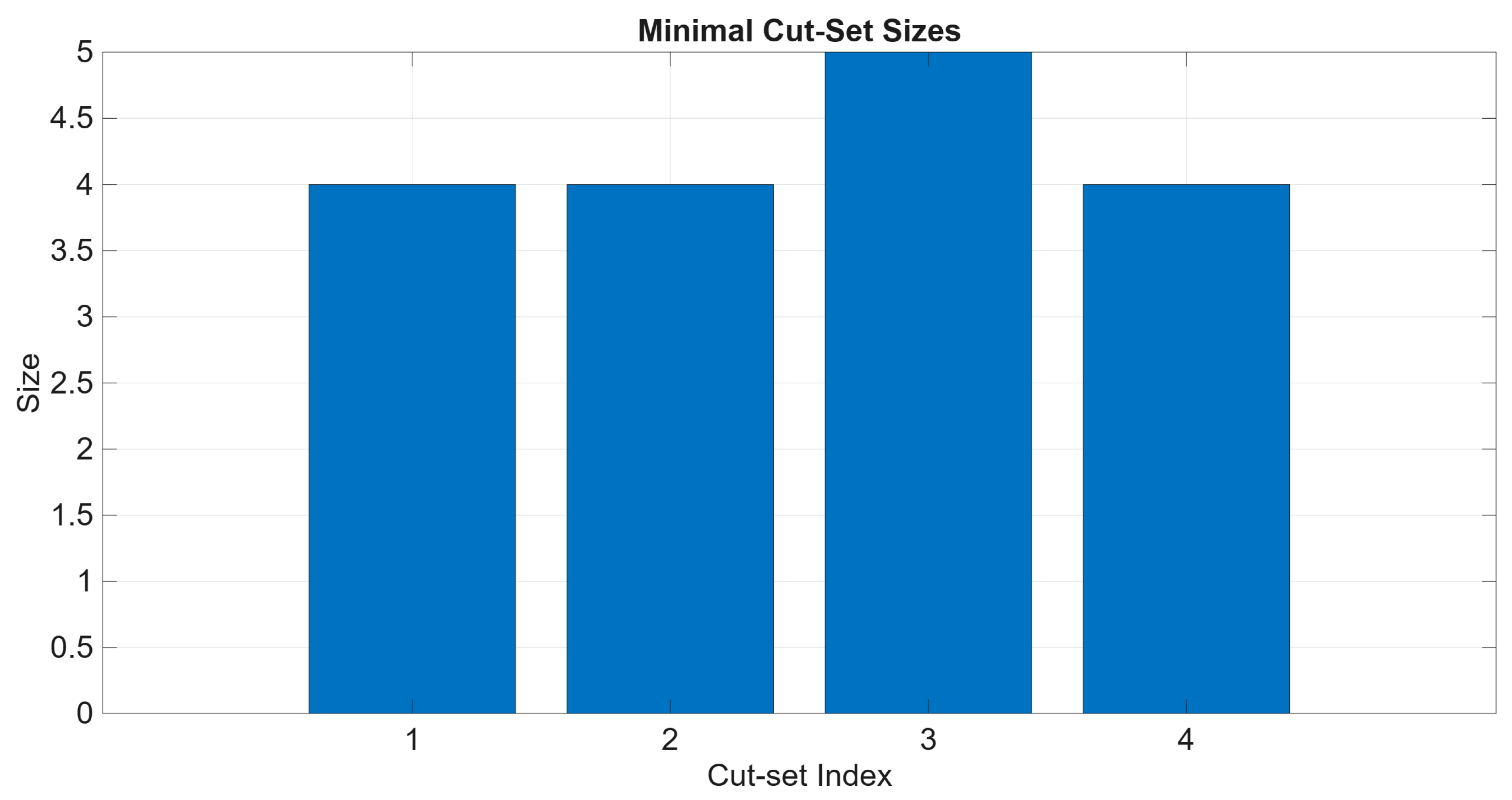
This section assesses the effectiveness of the proposed BowTie model, as outlined in Section 2.6.3. It examines this assessment through minimal cut sets, runtime performance, and model compactness. The traditional FTA yields four first-order minimal cut sets, as derived in Equation (24). This equation suggests that these single basic events alone could potentially trigger TE, indicating that their presence makes the system highly fragile. Conversely, the proposed BowTie-based analysis expands the FTA model beyond Boolean logic. It captures the interaction of barriers across both pathways. In this case study, the proposed model identifies four dominant cut-sets of order four or higher, which are 4, 4, 5, and 4, as displayed in Figure 14. This chart illustrates that multiple barriers must fail together for TE to propagate, reflecting more realistically the defence-in-depth principles embedded in engineered systems. While this illustrates the usefulness of BowTie in demonstrating resilience, this study acknowledges that the observed difference is specific to this case, and outcomes may differ for other subsystems or system architectures.

Figure 14. The number and size of the cut-set of the BowTie model.

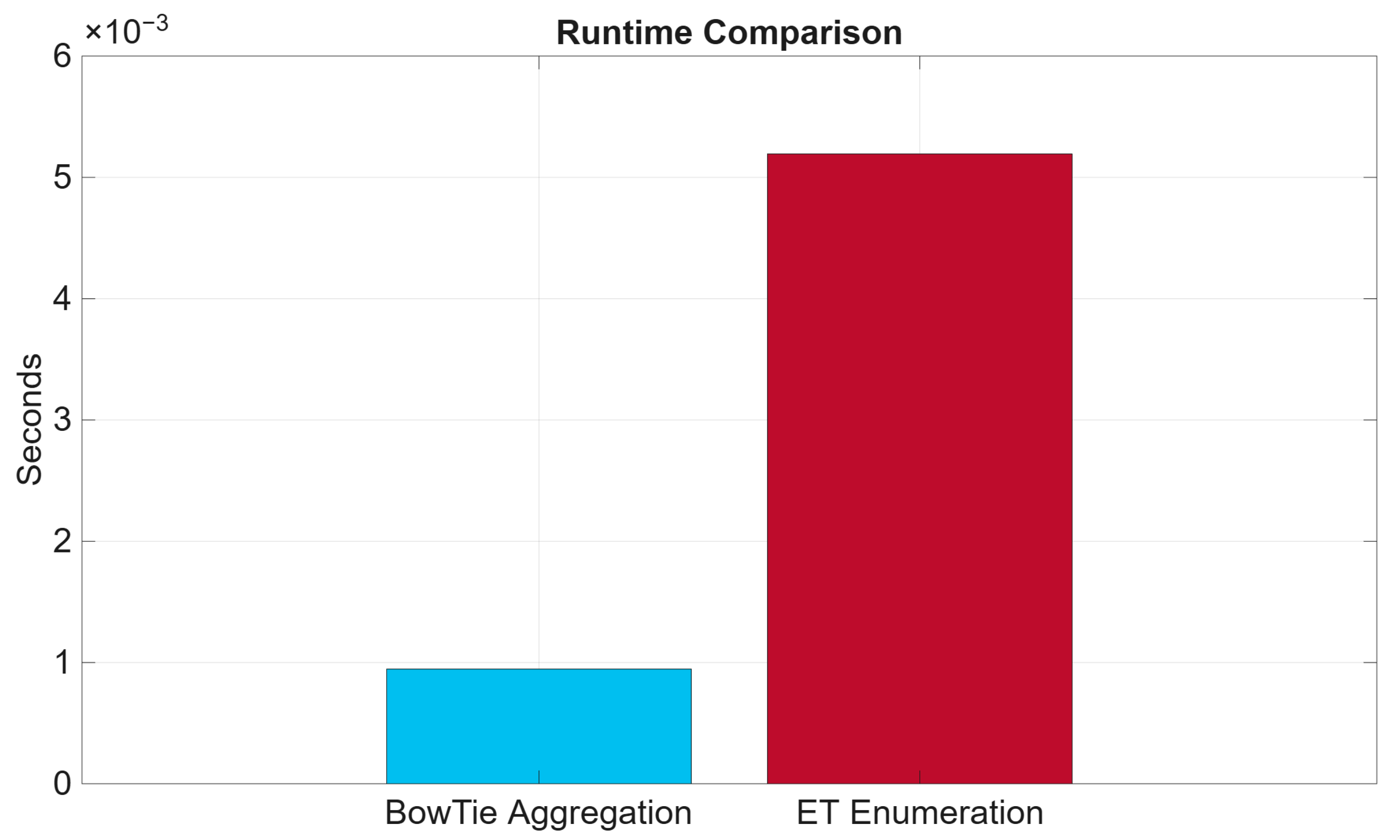
Another key feature of the BowTie model is its computational advantage, which is clear when comparing runtimes. Figure 15 shows that the BowTie aggregation method completes the task in around 0.0009 s, whereas full ETA enumeration takes 0.0729 s. This demonstrates that the framework can achieve efficiency gains while retaining analytical rigour. Although this case study involves a single subsystem, the results highlight the model’s potential for scaling to more complex systems where state-space growth poses a challenge.

Figure 15. A runtime comparison between the BowTie model and ETA.

Ultimately, the proposed BowTie model showcases its capability through its compact representation. As per Equations (18) and (19), the explicit ETA requires 64 distinct states to capture event sequences. In contrast, the BowTie model achieves the same analytical outcome using just 21 states, thereby eliminating 43 redundant states, as illustrated in Figure 16. This simplification of the BowTie model does not compromise analytical rigour, as evidenced by the value of Δ_f = 0.0000. While the state reduction achieved here is a clear advantage, the study notes that efficiency gains must always be balanced with the preservation of critical dependencies. In this case, the framework successfully maintained accuracy while improving compactness, underscoring its potential as a reliable yet efficient alternative to exhaustive enumeration.

Figure 16. Compactness comparison between BowTie and the ETA model.

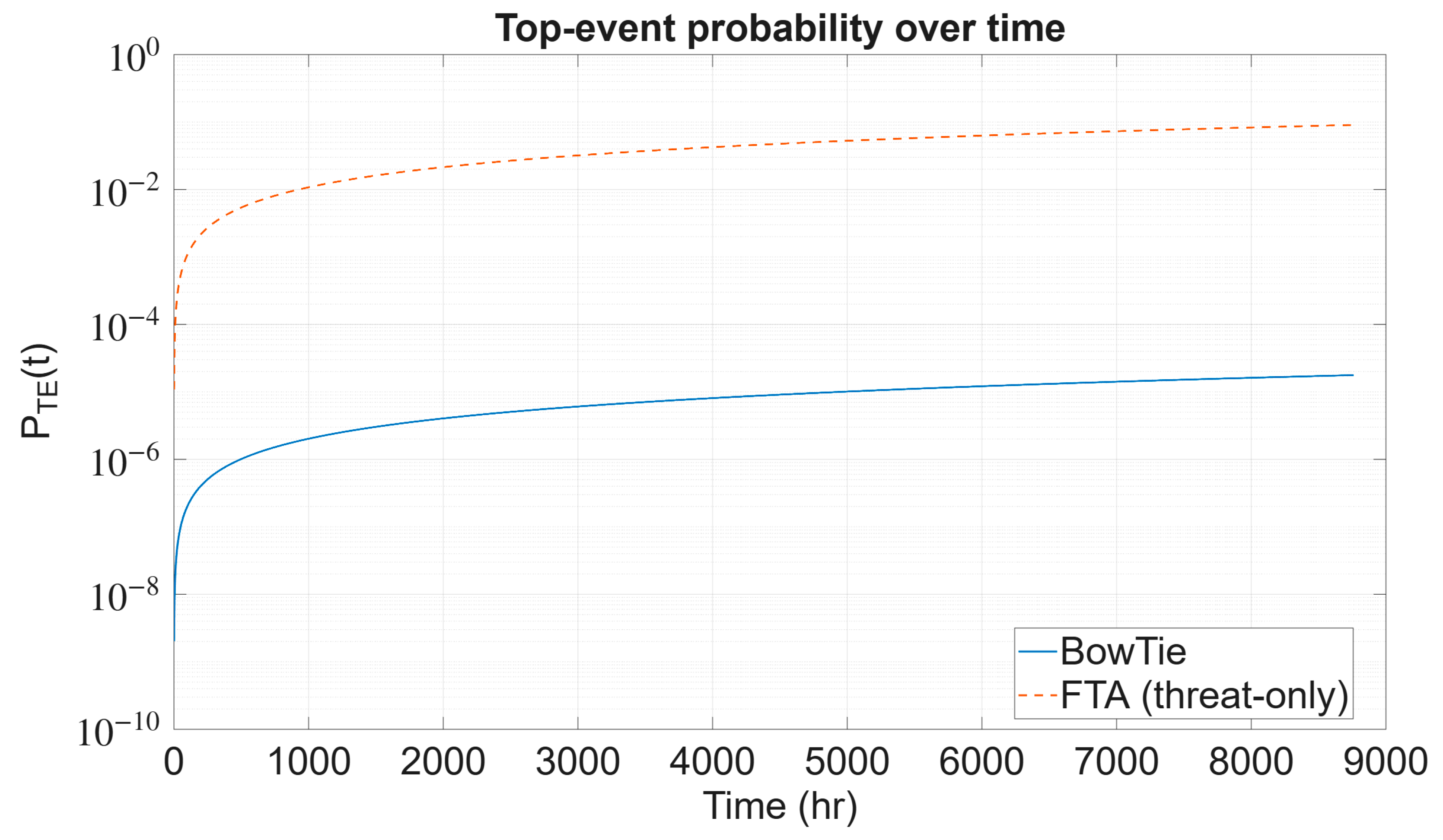
Another aspect of model comparison is the performance difference between the TE probability, ${\mathrm{P}}_{\mathrm{T}\mathrm{E}}\left(\mathrm{t}\right)$ estimated using the proposed BowTie framework with the conventional FTA (threat-only) approach. Figure shows the FTA curve (orange, dashed) rises sharply during the initial phase and quickly stabilises around 10⁻², reflecting the fragility implied when threats are modelled as direct precursors to the top event. In contrast, the BowTie curve (blue, solid) remains several orders of magnitude lower, stabilising in the range of 10⁻⁶–10⁻⁷ over the mission time. This outcome demonstrates the defence-in-depth effect: a top event occurs only when all associated preventive barriers fail, resulting in significantly reduced probabilities compared to the threat-only representation.

5. Discussions

The study answer the research question via four measurable outcomes: (i) risk contribution ranking using RAW and BIF (Figure 8 and Figure 9), (ii) quantified reliability improvements from scenario redesigns (Table 13; Figure 12 and Figure 13), (iii) quantitative evidence of barrier sufficiency over mission time (Figure 10 and Figure 11), and (iv) streamlined analysis relative to ETA/FTA (Figure 14, Figure 15 and Figure 16). The discussions presented in this section aim to interpret the main findings related to the research question in Section 1 and highlight their implications for system reliability and asset management.

5.1. Criticality of Barriers and Risk Contributions

The RAW findings in Section 4.1 emphasise significant variability in how individual barriers contribute to ${\lambda }_{\mathrm{T}\mathrm{E}}\left(\mathrm{t}\right)$. This inconsistency is clearly evident in key system components, such as sync-check relays and automatic trip triggers, which serve as single points of defence; their failure can directly cause system breakdown. Conversely, barriers like CBM dashboards and routine operator checks show a relatively low risk contribution to ${\lambda }_{\mathrm{T}\mathrm{E}}\left(\mathrm{t}\right)$. This suggests that removing these barriers would not significantly increase the ${\lambda }_{\mathrm{T}\mathrm{E}}\left(\mathrm{t}\right)$. Therefore, high-RAW barriers require strict routine maintenance, regular proof testing, and consideration of redundancy, while low-RAW barriers are optimised or rationalised depending on circumstances, such as operational costs.

Another important aspect of barrier contributions is the findings from BIF. It is essential to highlight that BIF analysis assumes barriers can either be perfected or improved. This implies that the probability of failure is negligible. According to BIF’s findings, all barriers at threat level L₀₇ could significantly lower ${\lambda }_{\mathrm{T}\mathrm{E}}\left(\mathrm{t}\right)$, contradicting the conclusions reached by RAW. There are several fundamental differences between the BIF and RAW analyses. BIF focuses on the advantages of enhancing a barrier, while RAW evaluates the potential damage that would occur if the barrier fails. A barrier that performs well (with a low P_fail) may have a low BIF (indicating limited room for improvement) but a high RAW (suggesting severe consequences if compromised), and the reverse can also be true. In practice, maintenance managers can use RAW to identify which barriers need maximum protection, while BIF helps justify investments by estimating the return on risk reduction [36]. For example, improving the oil analysis programme reduces the probability of failure from 0.72 to 0.20 and lowers ${\lambda }_{\mathrm{T}\mathrm{E}}\left(\mathrm{t}\right)$ by more than 70%, providing a clear business case for enhanced monitoring. By contrast, halving the proof-test interval for the automatic trip barrier has a negligible impact on risk, suggesting that resources would be better spent elsewhere.

These insights bridge the gap between technical analysis and financial decision-making. High-priority barriers (those with a high RAW) should be allocated greater inspection and testing budgets, as their failure would lead to prolonged outages and expensive repairs. In contrast, low-priority barriers may be grouped or de-scoped to save costs. BIF-driven improvements, such as upgrading vibration alarms or adopting more advanced oil-analysis sensors, can be compared against their implementation costs to evaluate the return on investment. This aligns with the broader reliability engineering literature, where risk-based inspection (RBI) and reliability-centred maintenance (RCM) frameworks are utilised to allocate maintenance resources based on both risk and cost considerations [36].

5.2. Reliability Improvements Through Barrier Redesign

The scenario-based sensitivity analysis in Section 4.4 reveals that not all preventive or mitigation strategies yield proportional gains. While redundancy and lowering barrier failure rates lead to significant reductions in system risk, as shown in Table 13, simply increasing proof-test frequency yields minimal additional benefit. In this case study, halving the auto-alarm proof-test interval reduced ${\mathrm{f}}_C\left(\mathrm{t}\right)$ by ≈0.03% (Table 13), indicating minimal marginal benefit versus redundancy or P_fail reduction. This outcome is consistent with modern reliability engineering and barrier management principles, which emphasise targeting the most influential safeguards rather than applying uniform maintenance escalation. For example, Yuan et al. [37] present a dynamic risk-informed safety barrier management approach where barrier interventions are prioritised based on current performance and risk contribution rather than scheduled intensification. Their method demonstrates that optimising high-leverage barriers yields more risk reduction per unit cost than blanket increases in inspection or testing intervals. Likewise, in the risk-based maintenance literature, Leoni et al. [38] compare various RBM methods and show that prioritisation based on probability × consequence offers more efficient resource allocation than across-the-board maintenance increases. Hence, the results of this study, where proof testing offers little marginal gain while barrier redesign and redundancy deliver considerable benefits, align with the principle of maintenance prioritisation by risk importance, reinforcing that strategic intervention wins over intensification. This prioritise-by-influence result mirrors risk-based barrier management and RCM guidance, which favour targeting high-leverage safeguards over blanket escalation of proof-testing or inspection intervals [39,40,41,42].

5.3. BowTie Modelling and Scalability

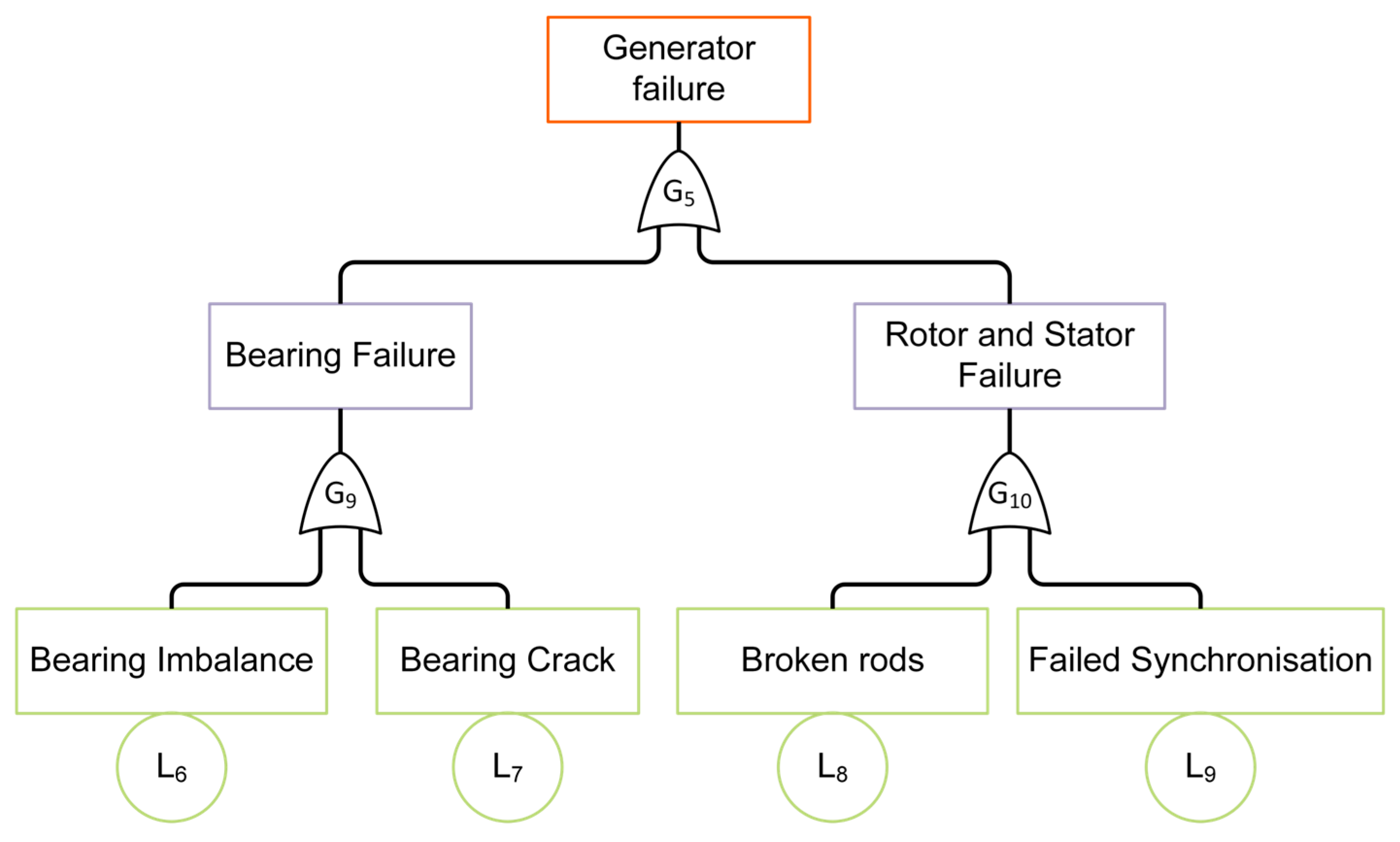
One of the key benefits of the proposed BowTie framework is its ability to simplify reliability modelling without compromising accuracy. This can be seen through the minimal cut set analysis, where the BowTie model can produce higher-order cut sets (size 4–5), requiring multiple barriers to fail to escalate the TE. In contrast, conventional FTA in Figure 5 generates first-order cut sets, suggesting that a single failure of basic events is enough to cause a catastrophic event. This difference indicates that the BowTie framework better reflects the defence-in-depth strategies used in practice, which capture the system’s resilience rather than exposing single-point vulnerabilities. Additionally, the BowTie model can reduce computational states compared to ETA enumeration without losing crucial detail. This means the proposed model has a high potential for scalability, making it suitable for larger or more complex systems where combinatorial explosion is a significant concern. This pattern is consistent with defence-in-depth guidance, where layered safeguards raise the minimum failure-combination order required for escalation.

5.4. Barrier Sufficiency over Mission Time

Investigating barrier sufficiency quantitatively shows that ${\lambda }_{\mathrm{T}\mathrm{E}}\left(\mathrm{t}\right)$, increases linearly but remains nearly constant over the mission period due to its small slope effect. The consequence frequency, ${\mathrm{f}}_{\mathrm{C}}\left(\mathrm{t}\right)$, on the other hand, remains at negligible levels, approximately 10⁻¹⁷/h. These findings provide strong evidence that the barrier configuration in the case study is sufficient to maintain reliability over the operating horizon. In practice, the defence-in-depth strategy ensures that even with gradual wear-out and ageing effects, the probability of escalation to severe consequences is effectively controlled and minimised, strengthening confidence in current operational practice.

5.5. Practical Implications and Generalisability

From an asset management perspective, this study highlights the benefits of a risk-informed approach to barrier design and maintenance prioritisation. The comparison in Figure 17 reinforces this point, as relying solely on FTA tends to overstate system fragility by overlooking the role of barriers. Incorporating preventive and mitigative defences through the BowTie framework demonstrates that the likelihood of generator failure is drastically reduced by several orders of magnitude over the mission duration. For example, the combined oil-analysis + dashboard scenario reduces ${\mathrm{f}}_{\mathrm{C}}\left(t\right)$ by 97.16% to 8.257 × 10⁻¹⁹ h⁻¹ (Table 16), illustrating the material impact of diagnostic upgrades on consequence frequency. For asset managers, this distinction is crucial because it clearly shows the value of barrier design and maintenance investments. Measures like trip relays, dashboards, and oil analysis directly lead to lower top-event risks. This approach thus supports risk-informed decisions, helping identify where resources should be focused and illustrating how defence-in-depth strategies offer meaningful improvements in reliability.

Figure 17. The performance difference of ${\mathrm{P}}_{\mathrm{T}\mathrm{E}}\left(t\right)$ estimated using the proposed model and FTA.

The proposed BowTie model thus offers decision-makers a structured approach to effectively balance safety and reliability by quantitatively ranking barriers, assessing the impacts of redesign, and verifying sufficiency. This approach aligns with risk-based inspection (RBI) by focusing maintenance resources on critical equipment while optimising inspection schedules to reduce operational costs without compromising safety [39,40]. Concerning the WT paradigm, the findings of this study indicate the importance of emphasising diagnostic redundancy and hybridisation, which lead to the most significant decrease in failure rates. Regarding the importance of barriers, critical protective relays, and automatic trip triggers significantly enhance overall system reliability when properly maintained. On the other hand, barriers that have a minimal impact can be optimised or streamlined to prevent unnecessary waste of resources. This viewpoint aligns closely with the principles of reliability engineering, which emphasise the importance of achieving the optimal level of system reliability by balancing risk reduction with economic practicality throughout the asset’s lifecycle [41].

Aside from the WT domain, the suggested BowTie methodology can also be applied to various critical infrastructures where a defence-in-depth approach is necessary to prevent a major incident. Yang et al. [42] showcase this approach by combining BowTie analysis with a Bayesian network to improve risk management in oil storage facilities. This enhances emergency response strategies and supports operational decision-making.

5.6. Limitations and Future Research

Several limitations of this study should be noted. First, the case study is limited to the generator subsystem of a WT, which constrains the generalisability of the findings; applying the framework to other subsystems or different infrastructures would provide broader validation. Second, the analysis relies on the assumption of constant failure rates for threats and barriers, without accounting for repair, degradation, or ageing effects. Similarly, HEPs and conditional probabilities are treated as fixed values, overlooking potential variability due to factors such as operator experience, fatigue, or context. Third, the data sources span multiple years and industries, including technical reports and cross-sector studies, which may introduce inconsistencies and reduce direct transferability to wind energy systems. Fourth, barrier independence is assumed, with dependencies and common-cause failures not explicitly considered. Fifth, the framework is presented deterministically, without quantifying uncertainty or providing error bounds for the reported results. Finally, efficiency gains over ETA are demonstrated for a single subsystem only; additional benchmarking on larger and more complex systems is required to substantiate scalability. In this paper, these assumptions are partially probed via scenario-based sensitivity, as explained in Section 3.4 and Section 4.4, to observe directional robustness of ${\lambda }_{\mathrm{T}\mathrm{E}}\left(\mathrm{t}\right)$ and ${\mathrm{f}}_C\left(\mathrm{t}\right)$ under barrier redesign.

Future research should build on this work by extending the framework to multiple subsystems and other critical infrastructures, incorporating non-constant failure behaviours such as repair and ageing, and refining the treatment of human and conditional probabilities to capture contextual variability. Explicit modelling of barrier dependencies and common-cause failures, together with validation against field data, would further enhance robustness. In addition, integrating uncertainty propagation techniques, such as Monte Carlo simulation or Bayesian inference, would enable the reporting of confidence intervals or error ranges, thereby strengthening interpretability. Finally, systematic benchmarking across larger case studies is needed to evaluate trade-offs between efficiency and accuracy, and to confirm the framework’s scalability for complex engineered systems.

6. Conclusions

This research has illustrated the BowTie framework based on reliability, which delivers a practical and effective method for quantifying system reliability, ranking barriers, and validating the adequacy of defence-in-depth measures. The framework provides a transparent and computationally efficient alternative to traditional reliability models, such as FTA, ETA, and RBD, by incorporating key metrics, including RAW and BIF, alongside cut-set analysis and scenario-based sensitivity evaluations. The findings indicate that high-risk barriers, such as protective relays and automation triggers, play a significant role in escalation pathways. In contrast, low-impact barriers exert only a marginal influence on overall system reliability. Furthermore, the higher-order cut sets generated by the proposed BowTie model provide a more realistic representation of the resilience of WT systems compared to the single-point vulnerabilities identified by conventional FTA.

The study also demonstrates significant efficiency gains: the BowTie model reduces runtime by approximately 40 times compared to ETA enumeration (0.0009 s vs. 0.0729 s) and compresses state requirements from 64 to 21 without loss of fidelity. These improvements highlight its potential for a scalable application. Nevertheless, several limitations remain. The current analysis is restricted to a single subsystem, assumes constant failure rates and barrier independence, and does not explicitly address common-cause failures or repair processes.

Future research should address these limitations by validating the framework across multiple WT subsystems and other infrastructures, incorporating non-constant failure behaviours (repair, ageing, degradation), and explicitly modelling dependencies between barriers. Large-scale benchmarking against conventional reliability techniques is also needed to assess scalability, computational trade-offs, and accuracy in complex engineered systems.