AI-Enhanced Virus Detection in Biopharmaceutical Production Processes

Abstract

Ensuring viral safety is a fundamental requirement in the production of biopharmaceutical products. Transmission Electron Microscopy (TEM) has long been recognized as a critical tool for detecting viral particles in unprocessed bulk (UPB) samples, yet manual counting remains labor-intensive, time-consuming, and prone to errors. To address these limitations, we propose an enhanced virus strain detection approach using the YOLOv11 deep learning framework, optimized with C3K2, SPPF, and C2PSA modules in the backbone, PANet in the neck, and Depthiwise Convolution (DWConv) in the head. To further improve feature fusion and detection of single-class virus particles, we integrated BiFPN and C3K2_IDWC modules. The resulting model (YOLOv11n + BiFPN + IDWC) achieves an mAP@0.5 of 0.995 with 33.6% fewer parameters compared to YOLOv11n, while increasing accuracy by 1.3%. Compared to YOLOv8n and YOLOv10n, our approach shows superior performance in both detection accuracy and computational efficiency. These results demonstrate that the model offers a robust and scalable solution for real-time virus detection and downstream process monitoring in the pharmaceutical industry.

1. Introduction

The detection and control of viral contaminants in biopharmaceutical processes are critical for ensuring product quality and patient safety [1,2]. Retroviruses such as murine leukemia virus (MLV) or xenotropic murine leukemia virus (X-MuLV) can contaminate mammalian cell substrates used for vaccines and therapeutic proteins, posing substantial biosafety risks [3]. Among current detection methods, Transmission Electron Microscopy (TEM) remains one of the most reliable tools for identifying viral contaminants, as it allows for direct visualization of viral particles without prior knowledge of the pathogen or specific reagents [4].

TEM is widely used to detect both known and emerging viral agents in unprocessed bulk (UPB) materials, making it an essential component of quality control during biologics manufacturing [5,6]. For example, TEM analysis of cell lines and viral harvests has proven effective in identifying retrovirus-like particles that may be invisible to infectivity assays. However, manual TEM analysis is time-consuming, requiring skilled operators and often taking hours to process a single batch of images, with a high risk of undercounting due to human fatigue [1,7].

Artificial intelligence (AI), particularly deep learning approaches, has recently shown great promise in automating virus detection from microscopy images [8,9]. The YOLO (You Only Look Once) object detection family is well known for ensuring real-time detection with high accuracy, making it an attractive choice for virus detection applications [10]. Studies have successfully applied CNN-based methods for detecting viral particles in TEM images, achieving near-perfect detection metrics [11]. Furthermore, the availability of benchmark TEM datasets and advancements in network architectures such as DenseNet201, ViResNet, and transformer-based models (e.g., VISN) have paved the way for more accurate and efficient virus detection pipelines [12,13,14].

In this work, we developed a YOLOv11-based virus detection system, enhanced by integrating BiFPN (Bidirectional Feature Pyramid Network) for multi-scale feature fusion and C3K2_IDWC for lightweight, morphology-adaptive detection. Our model was specifically designed for detecting retrovirus particles in UPB samples. We demonstrate that the proposed model significantly improves detection performance, reduces computational overhead, and provides reliable results for downstream virus safety testing in biopharmaceutical production.

2. Data Processing

2.1. Sample Collection and Preparation

The samples to be tested were first clarified by medium-low speed centrifugation and filtration, followed by ultra-high-speed centrifugation. The precipitate was resuspended in a fixed-volume solution, mixed with an equal volume of agar, then subjected to pre-fixation with glutaraldehyde and paraformaldehyde, post-fixation with tannic acid, and staining with uranyl acetate. The fixed samples underwent gradient dehydration and infiltration and were subsequently embedded in resin to form sample blocks after polymerization. The ultrathin sectioning technique was applied to section the samples, which were then fished onto copper grids, stained, and dried. Finally, the samples were examined and photographed under a transmission electron microscope.

2.2. Data Collection and Preprocessing

In the image processing stage, raw images were first screened to remove blurred ones and those without UPB virus strain cells, resulting in a total of 195 valid images. The labelimg tool was employed to annotate the UPB virus strain samples. During annotation, precise marking was conducted, targeting the morphological characteristics of the virus strains (such as spherical, rod-shaped, and irregular forms) and their residing backgrounds (including single-cell backgrounds, multi-cell overlapping backgrounds, and complex backgrounds with tiny impurities). After annotation, 10% of total, 19 images were selected as the test set, and the remaining images were divided into the training set and validation set at a ratio of 8:1. The training set was used for training the detection model, the validation set for adjusting model parameters and optimizing the model, and the test set for evaluating the model’s detection performance. To ensure the representativeness of the test set, consideration was given to virus strains with different morphologies and backgrounds when selecting the test set images, aiming to enhance the reliability of the detection results. Additionally, the image input size of the YOLOv11 network is 640 × 640, while the cell images obtained by computer scanning are 1095 × 866, which is larger than the network’s input size. Given that each image contains almost only one target and the YOLO network automatically resizes the input image to 640 × 640, no separate cropping was performed on the images in this study. In object detection, the production of training labels directly affects the quality of the final detection results. Therefore, it is necessary to create labels for UPB virus strain cells for each image. Figure 1 shows the process of preparation, electron microscopy imaging of UPB virus strain samples, and the training and validation of the detection model based on YOLOv11.

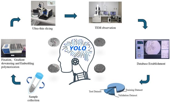
Figure 1. Process of preparation, transmission electron microscopy imaging of UPB virus strain samples and training and validation of detection model based on YOLOv11. This figure completely presents the entire process of UPB virus strain from sample preparation to label preparation. Firstly, in the sample preparation stage, a series of operations such as centrifugation, filtration, resuspension, fixation, staining, dehydration, embedding and sectioning are carried out to obtain samples that can be observed through a transmission electron microscope and complete the shooting. Then, in the image processing stage, 195 valid images are first screened out, and the labelimg tool is used to annotate them in combination with the morphological and background characteristics of the virus strains. After that, the images are divided into training set, validation set and test set according to the ratio of 8:1:1. Among them, the test set takes into account virus strains with different morphologies and backgrounds to ensure representativeness. Considering the input size of the YOLOv11 network and the target situation of the images, no cropping is performed on the images. Finally, the label preparation is completed, laying a foundation for subsequent work such as model training.

2.3. Sturcture of YOLOv11 Algorithm

The YOLO algorithm is a one-stage object detection algorithm that has become a well-known detection algorithm after multiple iterations. It is characterized by fast detection speed and high detection accuracy. This paper employs the YOLOv11 network to automatically detect viruses in UPB. The YOLOv11 model is a relatively new addition to the YOLO series. After receiving input, this model extracts image features through a convolutional neural network and detects targets by performing regression operations on the images. Its overall structure is shown in Figure 2.

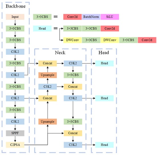
Figure 2. Overall structure diagram of YOLOv11. The YOLOv11 model, upon receiving input, extracts image features via a convolutional neural network and detects targets through regression operations on the image.

The YOLOv11 is consisted of section Backbone, section Neck and section Head. In the section Backbone, YOLOv11 uses the C3K2 module instead of the C2f module in YOLOv10. As shown in Figure 3, the C3K2 module is composed of multiple C3K modules. Through the superposition of multiple modules, information at different depths is extracted. The C3K module, in turn, contains multiple BottleNeck modules. Residuals can be optionally added to the BottleNeck modules. The residual adds the input and output of the BottleNeck, allowing the combination of shallow and deep information while increasing only a small amount of computational effort. This enhances the network’s feature extraction capabilities.

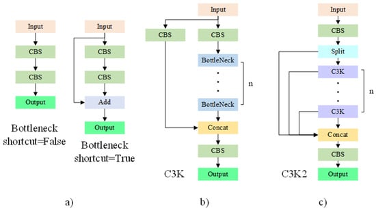
Figure 3. C3K2 Structure Diagram. The C3K2 module is composed of multiple C3K modules. It extracts information at different depths through the superposition of these modules. In turn, each C3K module contains multiple BottleNeck modules. It is optional to add residuals to the BottleNeck module, and the residuals will sum the input and output of the BottleNeck. (a) Bottleneck module, (b) C3k module, (c) C3K2 module.

In addition, YOLOv11 incorporates the SPPF module in the second-to-last layer of its backbone. This module is crucial for extracting multi-scale feature information. By stacking three max-pooling operations, it achieves feature fusion from local to global, further enhancing the information representation of feature maps and improving detection accuracy. The structure of the SPPF module is shown in Figure 4, where the kernel size of each max-pooling operation is 5 × 5.

Figure 4. SPPF structure diagram. YOLO11 incorporates the SPPF module in the second-to-last layer of its backbone. This module is crucial for extracting multi-scale feature information. It achieves feature fusion from local to global through the stacking of three maximum pooling operations, further enhancing the information expression of feature maps while improving detection accuracy. The kernel size of each maximum pooling operation is 5 × 5.

In the last layer of the backbone, YOLOv11 uses the C2PSA module. This module further enhances the model’s spatial attention capability through the stacking of multiple PSA modules, facilitating feature extraction by the network. The Attention module in the PSA module, inspired by Vision Transformer, introduces the attention mechanism from it to strengthen the network’s feature extraction. The structure diagram of C2PSA is shown in Figure 5.

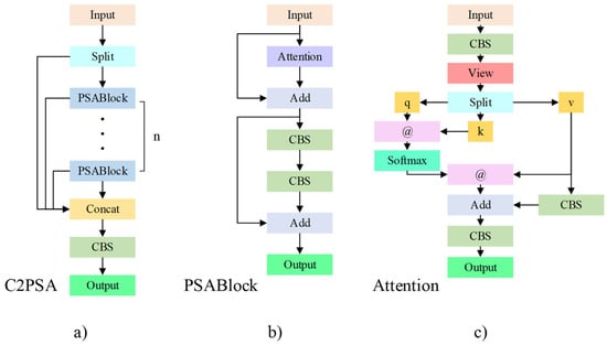
Figure 5. C2PSA structure diagram. The C2PSA module further enhances the model’s spatial attention capability through the stacking of multiple PSA modules, facilitating feature extraction by the network. (a) C2PSA module, (b) PSABlock module, (c) Attention module.

In the section Neck, YOLOv11 employs a Path Aggregation Network (PANet) to enhance feature extraction. During up sampling, the spatial dimensions of the feature maps are increased by interpolating between the pixels of the original feature maps. Here, nearest-neighbor interpolation is used to double the height and width of the feature maps before stacking them with the feature maps from the previous layer in the backbone. This enables communication between deep-layer and shallow-layer information and facilitates the transfer of deep-layer information to the shallow layers. After two rounds of up sampling and stacking, YOLOv11 performs down sampling. Down sampling reduces the height and width of the feature maps to half their original size through convolution. After reducing the feature maps, they are stacked with the feature maps from before the up sampling, further promoting the fusion of deep-layer and shallow-layer information.

In the section Head, compared to YOLOv10, YOLOv11 replaces the two CBS modules in the detection category loss with DWConv modules. DWConv is a depthwise separable convolution module that uses grouped convolution during convolution, with the number of groups being the greatest common divisor of the input and output channel numbers. This convolution effectively reduces redundant parameters and increases training efficiency.

2.4. The Improved YOLOv11

Given that traditional YOLOv11 is designed for multi-object detection, its application to a single category, such as retrovirus particles in UPB, leads to redundant parameters and computations. To address this, we simplified the YOLOv11 network while maintaining training accuracy, thus reducing the number of training parameters and improving efficiency.

We propose replacing the original PANet with BiFPN to significantly reduce network parameters. This modification optimizes feature fusion by enhancing cross-scale connections, akin to improvements in YOLOv5 where key modules such as feature fusion paths were optimized to reduce redundant computations while preserving feature representation [15]. BiFPN achieves efficient fusion by increasing node inputs and introducing bidirectional paths, thereby avoiding excessive feature extraction and aligning well with the single-class UPB virus dataset.

While PANet improves accuracy through down sampling, it demands more parameters and computational effort. For this study, given the relatively simple dataset structure, PANet would introduce unnecessary computational load. Therefore, we introduced the Weighted Bi-directional Feature Pyramid Network (BiFPN), which optimizes cross-scale feature fusion in traditional FPN. BiFPN allows each node to have multiple inputs, enhancing fusion efficiency. Additionally, for nodes with matching input-output layers, BiFPN adds an additional input from the backbone, enabling feature fusion without incurring significant cost. Unlike PANet, BiFPN’s bidirectional paths, treated as identical feature layers, are repeated multiple times to strengthen fusion. The BiFPN structure, shown in Figure 6, includes the Node_mode and Fusion modules. The Node_mode is composed of three C3K2 modules, each of which extracts features by stacking multiple C3K2 modules. The Fusion module generates trainable fusion weights, which are normalized and multiplied by the input feature maps to produce the final fused feature.

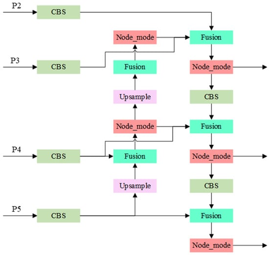
Figure 6. BiFPN module structure diagram. Each node in BiFPN has multiple inputs, which can improve the efficiency of feature fusion. Secondly, for nodes where the original input and output are at the same layer, BiFPN adds an additional input from the backbone part to fuse more features without incurring significant costs.

The irregular shapes of viruses and viral particles in the UPB dataset present challenges for traditional square convolution kernels. Conventional convolution fails to capture the complete target information, especially when the target occupies a small portion of the image, reducing model accuracy. Furthermore, redundant computations arise from processing a large number of similar channels. To mitigate this, we introduce the C3K2_IDWC module, which replaces some C3K2 modules to perform multi-scale convolution and reduce computational load. This approach, inspired by applications in agricultural disease detection [16], uses 3 × 3, 1 × 11, and 11 × 1 convolutions to adapt to irregular virus morphologies. The grouped convolution, with the number of groups set to 1/8 of the input channels, reduces redundant computations while enhancing the network’s ability to capture virus-specific features. The C3K2_IDWC structure, shown in Figure 7, includes two InceptionDWConv2d operations that divide input channels into four parts, with each part undergoing different convolutions to improve feature extraction. The final architecture replaces the last two C3K2 modules with C3K2_IDWC modules and replaces the PANet network with BiFPN. These improvements achieve a balance between lightweight design and high precision, consistent with the logic of optimizing YOLO for specific tasks [17]. The structure of the improved YOLOv11 network is shown in Figure 8.

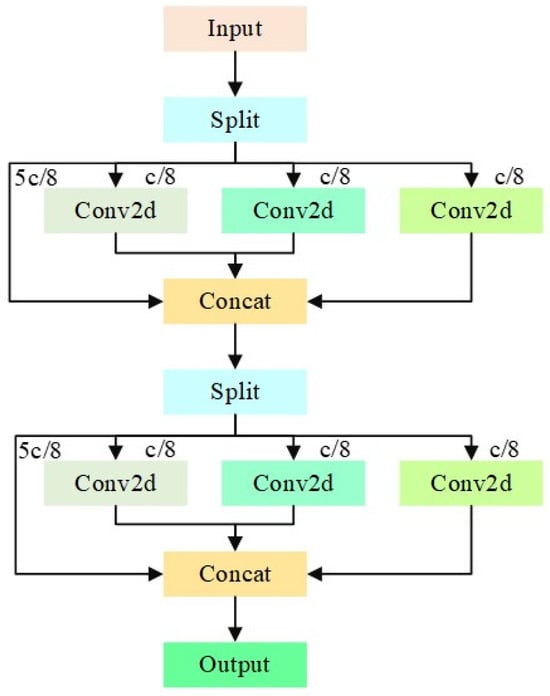
Figure 7. IDWC structure diagram. The input feature map consists of two InceptionDWConv2d operations. Each InceptionDWConv2d first divides the number of input channels into four parts: five-eighths of the channels remain unprocessed, while the remaining three groups of one-eighth channels undergo 3 × 3 convolution, 1 × 11 convolution, and 11 × 1 convolution, respectively. The number of groups for these convolutions is all set to one-eighth of the input channels. Finally, these results are stacked together.

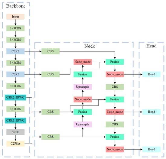
Figure 8. Improved YOLOv11. In the improved YOLOv11, PANet is replaced with BiFPN, which significantly reduces the number of network parameters. Additionally, the IDWC structure is introduced, which extracts features in different directions through multi-scale convolution and grouped convolution. This not only reduces the number of parameters but also enhances the feature extraction capability of the network.

3. Model Selection

Training Parameter Settings for YOLOv11, it was conducted using the Python 3.9 programming environment and the PyTorch 2.3.1 framework running on an NVIDIA GeForce RTX 3090 GPU (Wuxi, China). In the experiment, the SGD optimizer was used to facilitate the optimization of network parameters for the model. The momentum value was set to 0.937, the batch size was set to 4, and the number of training epochs was set to 100. Early stopping was triggered if the composite metric (calculated as 0.9 × mAP@0.5 + 0.1 × mAP@0.95) showed no improvement over 50 consecutive epochs.

In the YOLO object detection algorithm, detection accuracy is evaluated using the standard of mean Average Precision (mAP). Similarly to other machine learning models, the predicted results can be categorized into four scenarios: True Positives (TP), True Negatives (TN), False Positives (FP), and False Negatives (FN).

To calculate mAP, it is necessary to first compute Recall (R) and Precision (P). Recall is the ratio of the number of true positives to the total number of positive samples, which reflects the rate of missed detections of UPB virus strains. The formula for calculating Recall is as follows:

$$Recall={\displaystyle \frac{TP}{TP+FN}}$$

Precision is the ratio of true positives to all detected samples, which reflects the false detection situation of UPB virus strains. Its calculation formula is as follows:

$$Precision={\displaystyle \frac{TP}{TP+FP}}$$

Object detection algorithms typically use average precision (AP) and mean average precision (mAP) to assess the accuracy of model detection results. The AP measures the detection accuracy for a single target class by evaluating the trade-off between precision and recall. The MAP represents the meaning of all class AP values and is used to evaluate multiclass detection accuracy. It offers insight into the model’s performance across all classes. The calculation formula for MAP is as follows.

$$AP={\int }_0^{1}PRdR$$

$$MAP={\displaystyle \frac{1}{C}}\sum _{C_i\in C}A{P}_{\left(C_i\right)}$$

4. Results

The dataset was split into an 80% training set and a 10% validation set. The training set was used for model training, while the validation set was employed for parameter tuning.

4.1. Results of YOLOv11

As shown in Table 1, the proposed model achieves a 32.6% reduction in parameters compared to YOLOv11n, with a 1.3% improvement in accuracy, demonstrating optimal detection performance. To provide a comprehensive evaluation, the model was com-pared with YOLOv8 and YOLOv10. The results indicate that our model reduces the number of parameters by 42.2% and 35.3%, respectively, and decreases GFLOPs by approximately 25%, making it more suitable for deployment on resource-constrained devices. When compared with YOLOv11s, the proposed model matches its accuracy while requiring only 18.5% of the parameters, offering a more efficient solution without sacrificing performance. The model also demonstrates real-time inference capability, with each 640 × 640 image processed in less than 1 s on standard GPU hardware (NVIDIA RTX 3090), far exceeding the speed of manual TEM analysis.

Table 1. Model training results.

	GFLOPs	Parameter	Recall	Precision	mAP@0.5
YOLOv11n + BiFPN + IDWC	6.0	1.74M	1	0.954	0.995
YOLOv8n	8.1	3.01M	0.955	0.996	0.972
YOLOv10n	8.2	2.69M	0.981	0.915	0.983
YOLOv11n	6.3	2.58M	0.955	0.993	0.982
YOLOv11s	21.3	9.41M	1	0.952	0.991

4.2. Ablation Study and Impact of Individual Enhancements

Ablation experiments were performed to evaluate the contribution of each individual enhancement, as shown in Table 2. Integrating the BiFPN module alone reduced the parameter count by 25.6% while improving mAP@0.5 from 0.982 to 0.992. When the C3K2_IDWC module was introduced independently, parameters decreased by 8.4%, though the accuracy slightly fluctuated. Importantly, combining BiFPN and C3K2_IDWC led to a 32.6% total reduction in parameters while maintaining a high mAP@0.5 of 0.995, with precision reaching 0.954 and recall of 1.

Table 2. Ablation experiment results.

	GFLOPs	Parameter	Recall	Precision	mAP@0.5
YOLOv11n	6.3	2.58M	0.955	0.993	0.982
YOLOv11n + BiFPN	6.3	1.92M	0.946	1	0.992
YOLOv11n + IDWC	6.1	2.40M	0.948	1	0.986
YOLOv11n + BiFPN + IDWC	6.0	1.74M	1	0.954	0.995

These results clearly demonstrate that BiFPN effectively optimizes cross-scale feature fusion, while C3K2_IDWC enhances the extraction of irregular viral features. The synergy of these two enhancements not only compresses redundant parameters but also boosts detection precision. Representative detection outputs are illustrated in Figure 9, confirming the robustness and superior performance of the proposed model.

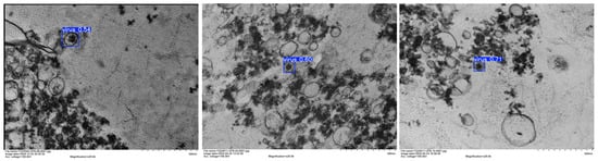
Figure 9. Detection result diagram. The improved YOLOv11 model performs excellently in detecting UPB virus strains, with mAP@0.5 reaching 0.995, a recall rate of 1, and a precision rate of 0.954. It has 1.74M parameters, a 32.6% reduction compared to YOLOv11n, and 6.0 GFLOPs, making it easy to deploy. Ablation experiments have verified the effectiveness of the improvements.

4.3. Noise Robustness Validation

To evaluate the model’s adaptability to suboptimal TEM images (a common scenario in biopharmaceutical QC, e.g., mild focus deviation, uneven staining), we conducted a dedicated robustness test using the experimental system established in this study, and referenced the annotations from Section 2.2 to count Total True Positives (TP), Total False Positives (FP, misdetections), and Total False Negatives (FN, undetected targets).

4.3.1. Experimental Process

To ensure the experiment’s reproducibility, we standardized the following key elements of the experimental process:

Test Data: We used the original 19-image test set (curated to cover diverse viral morphologies and backgrounds, Section 2.2) to avoid data leakage. Each image contains representative retrovirus-like particles, ensuring results accurately reflect real-world detection performance.

Disturbance Parameters: We selected Gaussian blur intensities that match common minor artifacts in industrial TEM sample preparation (e.g., slight focus deviation, thin-section thickness variation):

Convolution kernels: 3 × 3, 5 × 5, and 7 × 7. These sizes represent “mild to slightly obvious but still common” preparation errors—9 × 9 and larger kernels were excluded as they correspond to severe operational mistakes (e.g., extreme sectioning defects) that rarely occur in standardized QC workflows.

Experimental Protocol:

• Generated blurred images using OpenCV (v4.9.0), clipped to avoid image distortion (ensuring consistency with original TEM image format).
• Reused the final improved model (YOLOv11n + BiFPN + IDWC) with fixed inference parameters consistent with the original performance evaluation settings to eliminate parameter-induced metric biases.
• Conducted manual verification of all detection results: Each model output was cross-checked against the actual viral distribution in the test set (labeled via LabelImg in Section 2.2) to count true positives, false positives, and false negatives.

4.3.2. Quantitative Results

Key performance metrics under different Gaussian blur conditions are summarized in Table 3. All data reflect total statistics of the 19-image test set, aligning with batch detection scenarios in biopharmaceutical production.

Table 3. Noise robustness experiment results (Gaussian blur).

Disturbance Type	Disturbance Parameter	mAP@0.5 (Original: 0.995)	Recall (Original: 1.0)	Precision (Original: 0.954)	True Positives (TP)	False Positives (FP, Misdetected)	False Negatives (FN, Undetected)
Gaussian Blur	3 × 3 kernel	Cannot be calculated (Note 1)	1.0	0.864	19	3	0
Gaussian Blur	5 × 5 kernel	Cannot be calculated (Note 1)	1.0	0.864	19	3	0
Gaussian Blur	7 × 7 kernel	Cannot be calculated (Note 1)	1.0	0.864	19	3	0

Note 1: Reason for uncalculable mAP@0.5.

mAP@0.5 relies on the area under the Precision-Recall (P-R) curve, and generating a complete P-R curve requires multiple pairs of Precision-Recall values (typically obtained by adjusting the model’s confidence threshold). However, in this experiment:

• Under all Gaussian blur conditions (3 × 3, 5 × 5, 7 × 7 kernels), the model maintained a fixed Recall of 1.0 (all 19 true viral targets in the 19-image test set detected, FN = 0) and 3 false positives (FP = 3). This meant only one valid Precision value (19/(19 + 3) = 0.864) could be obtained, even with confidence threshold adjustments.
• Without sufficient pairs of Precision-Recall data to support P-R curve construction, traditional calculation of mAP@0.5 is not feasible.

4.3.3. Result Interpretation

Under all tested Gaussian blur conditions (3 × 3, 5 × 5, 7 × 7 kernels) on the 19-image test set, the model showed consistent performance characteristics:

Zero undetected batches: Total Recall remained 1.0 (all 19 true viral targets across the 19 images were detected), indicating the model’s strong ability to recognize viral features even when images are slightly blurred—fully meeting the biopharmaceutical QC requirement of “no missed contaminant detections in batch samples.”

Stable misdetection count: Total FP was consistently 3 (3 non-viral artifacts misdetected across the 19 images), leading to a Precision of 0.864 (down from the original 0.954). This stability suggests the model’s tolerance to blur (no increased misdetections with stronger blur) but also highlights a limitation: it cannot fully distinguish non-viral impurities from viruses under blurred conditions, which we have identified as a key direction for further optimization (e.g., adding an impurity classification branch).

5. Discussion

Viral safety is of paramount importance in biopharmaceutical production, particularly for biologics derived from mammalian cells. Retroviruses such as murine leukemia virus (MLV) and xenotropic murine leukemia virus (X-MuLV) can contaminate cell substrates, posing significant biosafety risks [4]. Transmission Electron Microscopy (TEM) serves as a key tool for detecting viruses in unprocessed bulk (UPB) samples, enabling direct visualization of viral particles without requiring prior knowledge of the pathogen [3]. Nevertheless, manual TEM analysis is time-consuming, taking 2–4 h to complete, and human fatigue may lead to undercounting or misjudgment issues that could delay production or result in missed contamination [7,18].

The improved YOLOv11 model (YOLOv11n + BiFPN + IDWC) presents a viable solution to these challenges. Boasting high accuracy with a mean Average Precision (mAP@0.5) of 0.995, it ensures reliable virus identification, thereby meeting regulatory requirements. With 1.74M parameters and 6.0 GFLOPs, it is compatible with standard laboratory equipment, striking a balance between detection accuracy and practical feasibility. For example, reducing TEM analysis from 2 to 4 h to <5 min per batch (with each image detected in <1 s) could shorten QC release timelines.

From a biological perspective, the model is well-adapted to the characteristics of viral particles in TEM images. The BiFPN module enhances cross-scale feature fusion, making it effective for identifying viruses of varying sizes within complex backgrounds. Meanwhile, the C3K2_IDWC module captures irregular viral morphologies through multi-scale convolutions, which contributes to its high precision (0.954) and recall (1). Notably, the noise robustness experiment (Section 4.3) further validates the model’s adaptability to the actual characteristics of TEM images. Under the conditions of 3 × 3, 5 × 5, and 7 × 7 Gaussian blurring (simulating common issues in industrial scenarios such as slight defocusing and uneven section thickness), the model’s Recall remained consistently at 1.0 (all 19 real viral particles were detected). This demonstrates that the cross-scale feature fusion capability of BiFPN can accurately anchor the core morphological features of viruses even when the viral edges are weakened due to blurring. Additionally, the multi-scale convolution (3 × 3, 1 × 11, 11 × 1) design of C3K2_IDWC effectively counteracts the interference of blurring on the morphological recognition of irregular viruses. This complements the detection performance under ideal conditions (Section 4.1), highlighting the model’s biological adaptability in non-ideal TEM workflows.

In practical applications, the model enables automated detection, processing image data within seconds and providing real—time results. This not only shortens quality control cycles but also allows for dynamic adjustments to downstream purification processes, minimizing production losses caused by detection delays. For a company producing 100 batches annually, the model saves 235 min per batch (240 min vs. 5 min), totaling 391.7 h (≈49 working days) of labor time each year. This reduction directly cuts manual TEM analysis costs and enables dynamic adjustments to purification processes, minimizing production delays. More crucially, accelerating QC cycles can expedite drug development: each month shortened in the time-to-market timeline for biopharmaceuticals can yield millions in revenue. By eliminating weeks of testing delays, the model has the potential to advance regulatory approval and earlier commercial launch by 3–6 months, delivering substantial competitive and financial advantages. As highlighted in recent industry analyses [19], early viral detection can avoid facility downtime and production delays, with the biomanufacturing viral detection market projected to grow at a CAGR of 8.2–9.37% through 2033 [2,5].

However, the study has certain limitations. The dataset, consisting of 195 images, covers a relatively narrow range of viral morphologies. In real-world scenarios, viruses may develop new morphological features due to changes in culture conditions or mutations, and the model’s ability to recognize such “unseen” morphologies remains untested. To address this, future work could expand the dataset by integrating TEM images of UPB samples containing viruses with diverse morphological variations—including those induced by controlled culture condition adjustments (e.g., temperature, nutrient concentration) and laboratory-simulated mutation models. Additionally, U-Net (a mainstream segmentation model) was not compared here as it targets semantic segmentation (evaluated via Dice coefficient), whereas our study focuses on object detection (evaluated via mAP); segmentation-based benchmarks will be included in future work if extending to virus quantification.

Additionally, the samples used are limited to monoclonal antibody intermediates derived from CHO cells; its adaptability to other cell lines or production processes requires further verification. This limitation may be mitigated by validating the model on UPB samples from a broader spectrum of biopharmaceutical production systems, such as those using HEK293 cells (for recombinant protein production) or Vero cells (for vaccine development), and across different manufacturing processes (e.g., batch, fed-batch, and continuous production).

Furthermore, Previously, the robustness of the model against actual TEM preparation artifacts had not been systematically evaluated. Although the newly added noise robustness experiment in this study (Section 4.3) has filled some gaps—verification through Gaussian blur on 19 test set images confirmed that the model is tolerant to minor disturbances (3 × 3~7 × 7 kernel) (Recall = 1.0). The experiment still has three limitations: first, the type of disturbance is single, only covering Gaussian blur, and does not involve more common artifacts in industrial scenarios such as uneven staining (e.g., uranyl acetate staining spots), copper mesh impurities (e.g., grid line interference), etc.; second, extreme disturbance scenarios (e.g., blur larger than 9 × 9, Gaussian noise with σ > 0.03) were not tested. Although such situations are rare in standardized QC, occasional preparation errors (e.g., overly thick ultra-thin sections) may still lead to a sudden drop in image quality; third, the fixed false detection problem found in the experiment (3 non-viral impurities were misjudged as viruses, Precision = 0.864) has not been resolved. This is because the C3K2_IDWC module is only designed for viral morphology and lacks targeted extraction of features of impurities such as cell debris and staining residues, which may trigger misjudged re-inspection of qualified batches in practical applications and increase production costs. To improve noise resilience, researchers could generate a dedicated noisy image subset by simulating common sample preparation artifacts (e.g., staining irregularities, debris accumulation, and sectioning defects) and fine-tune the model using this subset. Based on the results of this experiment, future optimizations can further focus on the following aspects: To address the issue of false detections, add a lightweight impurity classification branch in the model section Head. Train this branch using a small number of TEM impurity samples (such as CHO cell debris, tannic acid staining residues) to achieve accurate distinction between viral and non-viral features; at the same time, expand the interference type dataset, include uneven staining, copper mesh impurities, etc., in the robustness test, and integrate an adaptive wavelet denoising module to improve the model’s tolerance to extreme noise without adding excessive parameters (controlled within 2M). Alternatively, integrating a preprocessing module (e.g., adaptive median filtering or wavelet denoising) before the YOLOv11 detection pipeline could reduce the impact of extreme noise on detection performance.

6. Conclusions

This study developed an automatic detection scheme for UPB virus strain TEM images based on YOLOv11. Overall, 195 valid images were selected, annotated, and divided into test (19) and training/validation (176, 8:1) sets. Preprocessing was simplified via the model’s automatic size adjustment. With BiFPN replacing PANet for better feature fusion and C3K2_IDWC modules replacing backbone C3K2 to fit virus morphology and reduce computation, the improved model achieved 1.74M parameters (32.6% less than YOLOv11n), 6.0 GFLOPs, 0.995 mAP@0.5, 1 recall, and 0.954 precision. Matching YOLOv11s/YOLOv8n in accuracy but being more lightweight, it cuts detection time from 2 to 4 h to minutes with per-image inference under 1 s, enabling real-time QC in biopharmaceutical production. Future work will expand datasets and optimize noise resistance.

References

- Bullock, H.A.; Goldsmith, C.S.; Miller, S.E. Best practices for correctly identifying coronavirus by transmission electron microscopy. Kidney Int. 2021, 99, 824–827. [Google Scholar] [CrossRef] [PubMed]
- Guo, F. Application of electron microscopy in virus diagnosis and advanced therapeutic approaches. Viruses J. Histotechnol. 2024, 47, 1–4. [Google Scholar] [CrossRef] [PubMed]
- Roingeard, P.; Raynal, P.-I.; Eymieux, S.; Blanchard, E. Virus detection by transmission electron microscopy: Still useful for diagnosis and a plus for biosafety. Rev. Med. Virol. 2019, 29, e2019. [Google Scholar] [CrossRef] [PubMed]
- Nims, R.W. Detection of adventitious viruses in biologics—A rara occurrence. Dev. Biol. 2006, 123, 153–164. [Google Scholar]
- Roingeard, P. Viral detection using electron microscopy: 50 years of progress. Virus Res. 2018, 245, 3–9. [Google Scholar]
- De Sá Magalhães, S.; De Santis, E.; Hussein-Gore, S.; Colomb-Delsuc, M.; Keshavarz-Moore, E. Quality assessment of virus-like particle: A new transmission electron microscopy approach. Front. Mol. Biosci. 2022, 9, 975054. [Google Scholar] [CrossRef] [PubMed]
- Petkidis, A.; Andriasyan, V.; Yakimovich, A.; Georgi, F.; Witte, R.; Puntener, D.; Greber, F. Microscopy and deep learning approaches to study virus infections. iScience 2022, 25, 103812. [Google Scholar]
- Shiaelis, N.; Tometzki, A.; Peto, L.; McMahon, A.; Hepp, C.; Bickerton, E.; Favard, C.; Muriaux, D.; Andersson, M.; Oakley, S.; et al. Virus detection and identification in minutes using single-particle imaging and deep learning. ACS Nano 2023, 17, 697–710. [Google Scholar] [CrossRef] [PubMed]
- Andriasyan, V.; Yakimovich, A.; Petkidis, A.; Georgi, F.; Witte, R.; Puntener, D.; Greber, U.F. Microscopy deep learning predicts virus infections and reveals mechanics of lytic-infected cells. iScience 2021, 24, 102543. [Google Scholar] [CrossRef] [PubMed]
- Redmon, J.; Divvala, S.; Girshick, R.; Farhadi, A. You only look once: Unified, real-time object detection. In Proceedings of the 2016 IEEE Conference on Computer Vision and Pattern Recognition (CVPR), Las Vegas, NV, USA, 27–30 June 2016; pp. 779–788. [Google Scholar]
- Ito, E.; Sato, T.; Sano, D.; Utagawa, E.; Kato, T. Virus particle detection by convolutional neural network in transmission electron microscopy images. Food Environ. Virol. 2018, 10, 201–208. [Google Scholar] [CrossRef] [PubMed]
- Matuszewski, D.J.; Sintorn, I.-M. TEM virus images: Benchmark dataset and deep learning classification. Comput. Methods Programs Biomed. 2021, 209, 106318. [Google Scholar] [CrossRef]
- Kaphle, A.; Jayarathna, S.; Moktan, H.; Aliru, M.; Raghuram, S.; Krishnan, S.; Cho, S.H. Deep learning-based TEM image analysis for fully automated detection of gold nanoparticles internalized within tumor cell. Microsc. Microanal. 2023, 29, 1474–1487. [Google Scholar] [CrossRef] [PubMed]
- Xiao, C.; Wang, J.; Yang, S.; Heng, M.; Su, J.; Xiao, H.; Song, J.; Li, W. VISN: Virus instance segmentation network for TEM images using deep attention transformer. Brief. Bioinform. 2023, 24, bbad373. [Google Scholar] [CrossRef] [PubMed]
- Zhang, X.; Min, C.; Luo, J.; Li, Z. YOLOv5-FF: Detecting Floating Objects on the Surface of Fresh Water Environments. Appl. Sci. 2023, 13, 7367. [Google Scholar] [CrossRef]
- Liu, J.; Wang, X. Improved YOLOv3 for tomato pest detection using multi-scale feature fusion. Comput. Electron. Agric. 2020, 175, 105–113. [Google Scholar]
- Sharma, J.; Kumar, M.; Pradhan, S.; Chattopadhay, S.; Kukreja, V.; Verma, A.A. YOLO-Based Framework for Accurate Identification of Wheat Mosaic Virus Disease. Comput. Biol. Chem. 2024, 83, 107424. [Google Scholar]
- Goldsmith, C.S.; Miller, S.E. Modern uses of electron microscopy for detection of viruses. Clin. Microbiol. Rev. 2009, 22, 552–563. [Google Scholar] [CrossRef] [PubMed]
- Kouassi, M.-A. Genedata. Faster, Safer, More Comprehensive Viral Detection in Biologics Manufacturing. 2022. Available online: https://www.genedata.com/news/details/comprehensive-viral-detection-in-biologics-manufacturing (accessed on 15 May 2025).
Disclaimer/Publisher’s Note: The statements, opinions and data contained in all publications are solely those of the individual author(s) and contributor(s) and not of MDPI and/or the editor(s). MDPI and/or the editor(s) disclaim responsibility for any injury to people or property resulting from any ideas, methods, instructions or products referred to in the content. |
© 2025 by the authors. Licensee MDPI, Basel, Switzerland. This article is an open access article distributed under the terms and conditions of the Creative Commons Attribution (CC BY) license (https://creativecommons.org/licenses/by/4.0/).