Internal Force Analysis of Circular Shaft Structures Considering Spatial Arching and Interlayer Shear Effects

Abstract

To accurately investigate the stress and deformation behavior of support structures during mechanical shaft construction, this study proposes an analytical method for active earth pressure calculation based on limit equilibrium theory, incorporating both the radial variation of the circumferential stress coefficient and the spatial arching effect. Considering the entire sliding soil mass behind the shaft wall as the analytical object, the inclination angle of the sliding surface under active limit conditions is derived. Subsequently, by incorporating interlayer shear forces, a horizontal layer analysis is employed to establish the vertical and radial force equilibrium equations, leading to the formulation of an active earth pressure model for circular shafts. Furthermore, based on elastic mechanics theory, a corresponding method is developed to calculate the internal forces of the shaft structure. The theoretical predictions show good agreement with existing model test results and field monitoring data, demonstrating the accuracy and reliability of the proposed approach. The findings provide a theoretical basis for optimizing the design of circular shafts and assessing the structural stability of shaft walls.

1. Introduction

As an emerging shaft construction technique, the mechanized shaft method integrates undrained excavation, overall suspended sinking, mechanical cutting using a milling drum, and prefabricated shaft assembly. This method exhibits strong adaptability to weak, disturbed, or otherwise unstable ground conditions. It significantly mitigates the impact of shaft construction on the surrounding strata, while reducing construction time and overall cost. Owing to these advantages, it has been increasingly adopted in modern shaft engineering practice.

Similar to other underground structures, mechanized shafts are inevitably subjected to earth and rock pressures from the surrounding strata, resulting in stress and deformation of the support system. Therefore, accurate estimation of the earth pressure acting on the support structure is essential in the structural design process. The classical Rankine and Coulomb earth pressure theories are widely applied in engineering practice due to their simplicity. However, their assumption of a linear earth pressure distribution often deviates from actual field conditions, leading to discrepancies between the theoretical and measured resultant earth pressures. Numerous laboratory tests have demonstrated that the active earth pressure behind plane retaining walls exhibits a nonlinear distribution [1,2]. Model tests on circular shafts have further confirmed this nonlinearity, revealing significant deviations from the classical Rankine earth pressure predictions [3].

In recent years, extensive research has been carried out by both domestic and international scholars on the distribution of earth pressure behind retaining walls. Current analytical approaches for evaluating earth pressure on plane retaining walls primarily include the limit equilibrium method, slip-line theory, and limit analysis. Among these, the limit equilibrium method based on horizontal layer analysis has been widely adopted and has yielded numerous valuable results. For example, Handy [4], Paik and Salgado [5], as well as Goel and Patra [6], incorporated the soil arching effect in the backfill and, based on the horizontal layer analysis method, derived the nonlinear distribution of active earth pressure in sandy soils. Since then, the earth pressure calculation method combining horizontal layer analysis with the soil arching effect has been further extended to various conditions, including seismic loading, limited-width backfills, seepage effects, and curved failure surfaces [7,8,9,10,11,12]. These developments have significantly advanced the understanding of earth pressure on plane retaining walls. Compared with the extensive research on plane retaining walls, studies on the calculation of earth pressure acting on curved retaining structures (e.g., circular shafts) remain relatively limited. Terzaghi [13] was among the first to consider the effects of soil friction angle and the height-to-diameter ratio. Following an approach similar to Coulomb’s earth pressure theory, he derived an expression for the earth pressure on circular shafts based on the overall static equilibrium of the sliding soil mass. However, numerous studies have shown that under limit equilibrium conditions, stress redistribution in the soil behind the shaft gives rise to a vertical arching effect, similar to that observed in plane retaining walls. Additionally, a horizontal circular arching effect also develops. These two mechanisms, collectively referred to as the spatial arching effect, significantly influence both the magnitude and distribution of earth pressure [14,15].

To account for the influence of the circumferential arching effect, Berezantzev [16] adopted the Haar–Karman assumption, which assumes that the circumferential stress ${\sigma }_{\theta }$ is always equal to the major principal stress ${\sigma }_1$, and applied slip-line theory to derive the active earth pressure acting on circular shafts. However, subsequent studies [17,18,19] have shown that the Haar–Karman assumption tends to overestimate the contribution of circumferential stress, as confirmed through extensive analytical and experimental investigations. For example, Prater [17] introduced the concept of a circumferential stress coefficient $\lambda$, defined as the ratio of circumferential stress to the major principal stress, and proposed that it should be taken as the static earth pressure coefficient K₀. Using the limit equilibrium method, he derived a formula for calculating the active earth pressure while accounting for the circumferential arching effect. The calculated results showed good agreement with experimental data in shallow soils but deviated significantly at greater depths. Furthermore, some researchers have considered both vertical and circumferential arching effects simultaneously. For instance, Chen and Zhou [20] and Lu et al. [21] incorporated the spatial arching effect and developed active earth pressure formulations for circular retaining walls based on the limit equilibrium approach. Zhang et al. [22,23] developed a calculation model for active earth pressure under various shaft wall displacement modes based on the horizontal layer analysis method, incorporating the influence of the spatial arching effect. Jia et al. [24] adopted the Coulomb failure mechanism and derived a formulation for active earth pressure in circular shafts using the energy method, accounting for energy dissipation induced by circumferential stress. Recognizing that shaft wall displacement in practical applications is often insufficient to mobilize the active limit state, Pedro [25] proposed a non-limit active earth pressure model that explicitly considers shaft wall displacement effects.

Most of the aforementioned studies assume that the circumferential stress coefficient $\lambda$ remains constant. However, its magnitude is, in fact, strongly dependent on the spatial location of the soil element [26,27]. Based on discrete element simulations, Chen and Zhou [28] observed that the circumferential arching effect diminishes progressively with increasing distance from the wall, leading to a corresponding decrease in the circumferential stress coefficient $\lambda$. Similarly, Xiong et al. [29,30] analytically derived the circumferential stress under axisymmetric active limit conditions and concluded that the influence of the circumferential arching effect decreases with radial distance. Therefore, assuming a constant circumferential stress coefficient inevitably introduces significant discrepancies between calculated and actual earth pressure distributions [31]. In addition, due to the presence of soil arching in the vertical plane, the principal stress direction undergoes rotation, which induces horizontal shear stresses. These shear stresses significantly affect both the magnitude of the active earth pressure and the location of its resultant force [32,33]. However, this effect has not been adequately addressed in existing studies on shaft earth pressure.

Based on the above analysis, this study investigates the sliding soil mass behind the shaft wall, taking into account the radial variation of the circumferential stress coefficient. An analytical expression for the inclination angle of the sliding surface under active limit state conditions is derived. Incorporating the effects of spatial soil arching and interlayer shear, a calculation method for active earth pressure is established using a horizontal layer analysis approach combined with vertical and radial static equilibrium conditions. The proposed equation is validated through comparison with existing theoretical models and experimental results. Furthermore, an internal force calculation method for the shaft lining is developed based on elastic theory, considering the spatial effects of soil arching and interlayer shear. The proposed method is verified against field monitoring data, demonstrating its accuracy and practical applicability.

2. Analysis and Derivation of the Inclination Angle of the Sliding Surface Behind the Shaft Wall

2.1. Analytical Model and Basic Assumptions

Figure 1 presents the analytical model of soil sliding behind the circular shaft wall, where the shaft has a radius r₀ and a depth H. The fundamental assumptions employed in the calculations are as follows:

(1) Although numerous experimental studies have demonstrated that the sliding surface of soil at the active limit state is curved, existing research indicates that the theoretical earth pressure values calculated using a curved sliding surface and those based on the Coulomb planar sliding surface differ only slightly (approximately 6%). Moreover, the results obtained with the Coulomb planar sliding surface are generally more conservative [12]. Considering computational complexity and practical engineering applicability, this study assumes that the sliding surface is planar; specifically, the slip line is taken as a straight line passing through the heel of the wall, with an inclination angle of $\beta$.

(2) The shaft wall is assumed to be rough, the backfill behind the shaft wall consists of clay, the backfill surface is horizontal, and the external load is uniformly distributed. Additionally, the influence of interlayer shear stress within the soil is considered.

(3) The displacement mode of the shaft wall is assumed to be translational.

2.2. Establishment of the Equilibrium Equation and Determination of the Sliding Surface Inclination Angle

The entire sliding soil mass behind the shaft wall is taken as the research object (see Figure 1), and its vertical and horizontal force components are illustrated in Figure 2. In the figure, $F_{\phi }$ denotes the force exerted by the soil outside the sliding surface on the sliding soil mass, with an angle $\phi$ relative to the normal of the sliding surface (i.e., the internal friction angle of the soil), and the radial coordinate at the point of action is $r_1$. $F_{\delta }$ represents the force applied by the shaft wall to the sliding soil mass, forming an angle $\delta$ with the horizontal plane (i.e., the wall-soil friction angle). $F_{c_{\mathrm{w}}}$ and $F_c$ are the resultant cohesive forces at the wall–soil interface and along the sliding surface, respectively. $F_q$ is the resultant force generated by the uniformly distributed load on the backfill surface, $G$ represents the self-weight of the sliding soil mass, and $F_{\theta }$ is the resultant force of the circumferential stress acting on the sliding soil mass.

Based on the analysis of Figure 2, the static equilibrium equations for the sliding soil mass in the vertical and horizontal directions can be expressed as:

$$2\pi \left[F_{\delta }\sin \delta \cdot r_0+F_{\phi }\cos (\beta -\phi )\cdot r_1\right]+F_c\sin \beta +F_{c_{\mathrm{w}}}=G+F_q$$

(1)

$$F_{\delta }\cos \delta \cdot r_0\mathrm{d}\theta +2F_{\theta }\sin \left({\displaystyle \frac{\mathrm{d}\theta }{2}}\right)+F_c\cos \beta \cdot {\displaystyle \frac{\mathrm{d}\theta }{2\pi }}=F_{\phi }\sin (\beta -\phi )\cdot r_1\mathrm{d}\theta$$

(2)

Since the value of $\mathrm{d}\theta$ is relatively small, it can be reasonably approximated as $\sin \left({\displaystyle \frac{\mathrm{d}\theta }{2}}\right)\approx {\displaystyle \frac{\mathrm{d}\theta }{2}}$. By further combining Equations (1) and (2), the following expression can be obtained:

$$F_{\delta }={\displaystyle \frac{\sin (\beta -\phi )}{2\pi r_0\cos (\beta -\phi -\delta )}}\left\{G-\left[2\pi \cot (\beta -\phi )\right]F_{\theta }-\left[\sin \beta +\cos \beta \cot (\beta -\phi )\right]F_c-F_{c_{\mathrm{w}}}+F_q\right\}$$

(3)

Since the Haar–Karman assumption tends to overestimate the influence of circumferential stress, Prater [17] introduced the circumferential stress coefficient $\lambda$ (i.e., ${\sigma }_{\theta }=\lambda {\sigma }_1$), suggesting that its value should range between 1 and K₀. From the perspective of engineering safety, Prater recommended adopting K₀ (where K₀ denotes the coefficient of static earth pressure). However, existing studies have demonstrated that as the radial distance from the shaft wall increases, the influence of the circumferential arching effect progressively diminishes, leading to a corresponding decrease in circumferential stress. The magnitude of the circumferential stress coefficient $\lambda$ is strongly dependent on the radial distance: near the shaft wall, the coefficient approaches 1, whereas near the sliding surface, it tends toward K₀ [28,30].

For computational convenience, it is assumed that the circumferential stress decreases linearly along the radial direction, meaning that the circumferential stress coefficient $\lambda$ varies linearly with the radial coordinate r:

$$\lambda =1-(1-K_0)\left({\displaystyle \frac{r-r_0}{r_{\beta }-r_0}}\right)$$

(4)

where K₀ is the static earth pressure coefficient, and $K_0=1-\sin \phi$; $r_{\beta }$ represents the radial coordinates at the sliding surface.

The average circumferential stress coefficient $\overline{\lambda }$ of the horizontal differential element at any height under the active limit state can be determined using Equation (4):

$$\overline{\lambda }={\displaystyle \frac{1+K_0}{2}}$$

(5)

Further, the average circumferential stress coefficient ${\sigma }_{\mathrm{a}\theta }$ of the horizontal differential unit can be expressed as:

$${\sigma }_{a\theta }=\overline{\lambda }{\sigma }_1=\left({\displaystyle \frac{1+K_0}{2}}\right)(\gamma z+q)$$

(6)

The circumferential force $F_{\theta }$ can ultimately be obtained from Equation (6):

$$F_{\theta }={\displaystyle {\int }_0^H{\sigma }_{\mathrm{a}\theta }\left(\frac{H-z}{\tan \beta }\right)} \mathrm{d}z={\displaystyle \frac{(1+K_0)(\gamma H+3q)H^2}{12\tan \beta }}$$

(7)

The self-weight G of the sliding soil mass behind the shaft wall is given by:

$$G=\gamma V=\gamma {\displaystyle {\int }_0^H\pi }\left[{\left(r_0+{\displaystyle \frac{H-z}{\tan \beta }}\right)}^2-{r_0}^2\right]\mathrm{d}z={\displaystyle \frac{\pi \gamma H^2}{\tan \beta }}\left(r_0+{\displaystyle \frac{H}{3\tan \beta }}\right)$$

(8)

In addition, the values of the other pertinent parameters are summarized as follows:

$$\left\{\begin{array}{l}{F}_{c_{\mathrm{w}}}=c_{\mathrm{w}}{S}_{c_{\mathrm{w}}}=2\pi c_{\mathrm{w}}{r}_{0}H\hfill \\ F_c=c{S}_c={\displaystyle \frac{\pi cH(2r_0+H\cot \beta )}{\sin \beta }}\hfill \\ F_q=q{S}_q=\pi qH\cot \beta (2r_0+H\cot \beta )\hfill \end{array}\right.$$

(9)

where $c_{\mathrm{w}}$ and $c$ represent the cohesion at the wall–soil interface and the cohesion of the soil, respectively $c_{\mathrm{w}}=c(\tan \delta /\tan \phi )$; $q$ represent the uniformly distributed load acting on the fill surface; $S_{c_{\mathrm{w}}}$, $S_c$, and $S_q$ denote the action areas corresponding to the forces mentioned above.

Based on Coulomb’s earth pressure theory, Equations (7)–(9) are substituted into Equation (3), and the extremum (i.e., parameter $\mathrm{d}{F}_{\delta }/\mathrm{d}\beta =0$) is determined, which can be readily solved using MATLAB (R2023b, The MathWorks, Inc., Natick, MA, USA). Details are omitted here for brevity.

Accordingly, the inclination angle of the soil sliding surface under the active limit state is obtained. This angle is influenced by multiple factors, including the internal friction angle of the soil, the wall–soil friction angle, the soil cohesion, the uniformly distributed load on the fill surface, and the shaft radius-to-height ratio.

$$\beta =f\left(\phi , \delta , c, q, {\displaystyle \frac{r_0}{H}}\right)$$

(10)

Unlike the traditional planar earth pressure theory, Equation (10) more precisely captures the effect of the radius-to-height ratio on the inclination angle of the sliding surface.

2.3. Comparative Validation and Analysis of Influencing Factors

Figure 3a illustrates the variation of the sliding surface inclination angle with the radius-to-height ratio under the given conditions and compares the calculation results of this study with the Coulomb theory values and the results reported by Lu et al. [21].

As shown in the figure, compared with the plane retaining wall, the sliding surface inclination angle in the circular shaft is significantly influenced by the radius-to-height ratio. When the radius-to-height ratio is less than 15, the sliding surface inclination angle in the circular shaft is greater than that predicted by Coulomb’s theory, and the smaller the radius-to-height ratio, the more pronounced the difference between the two. In addition, the sliding surface inclination angle decreases as the radius-to-height ratio increases and gradually approaches the Coulomb solution. Furthermore, a larger wall–soil friction angle results in a smaller sliding surface inclination angle for the same radius-to-height ratio. Finally, the calculation results of this study show good agreement with the values reported by Lu et al. [21], thereby verifying the rationality of the proposed calculation method.

Figure 3b further illustrates the relationship between the sliding surface inclination angle and soil cohesion. As shown in the figure, with an increase in soil cohesion, the sliding surface inclination angle also increases, but the rate of increase gradually slows down. Moreover, the smaller the internal friction angle of the soil, the more significant the effect of soil cohesion. This is because, as soil cohesion increases, it becomes necessary to generate sufficient shear stress in the soil with higher cohesion to satisfy the limit equilibrium condition, thereby initiating active failure. This, in turn, leads to an increase in the sliding surface inclination angle.

3. Analysis of Active Earth Pressure in Circular Shafts

This study simultaneously considers the vertical arching effect and circumferential arching effect (i.e., the spatial arching effect) generated by the soil behind the shaft wall during deformation and incorporates the shear stress between horizontal soil layers to determine the active earth pressure distribution behind the circular shaft wall using the horizontal layer analysis method.

3.1. Vertical Arching Effect

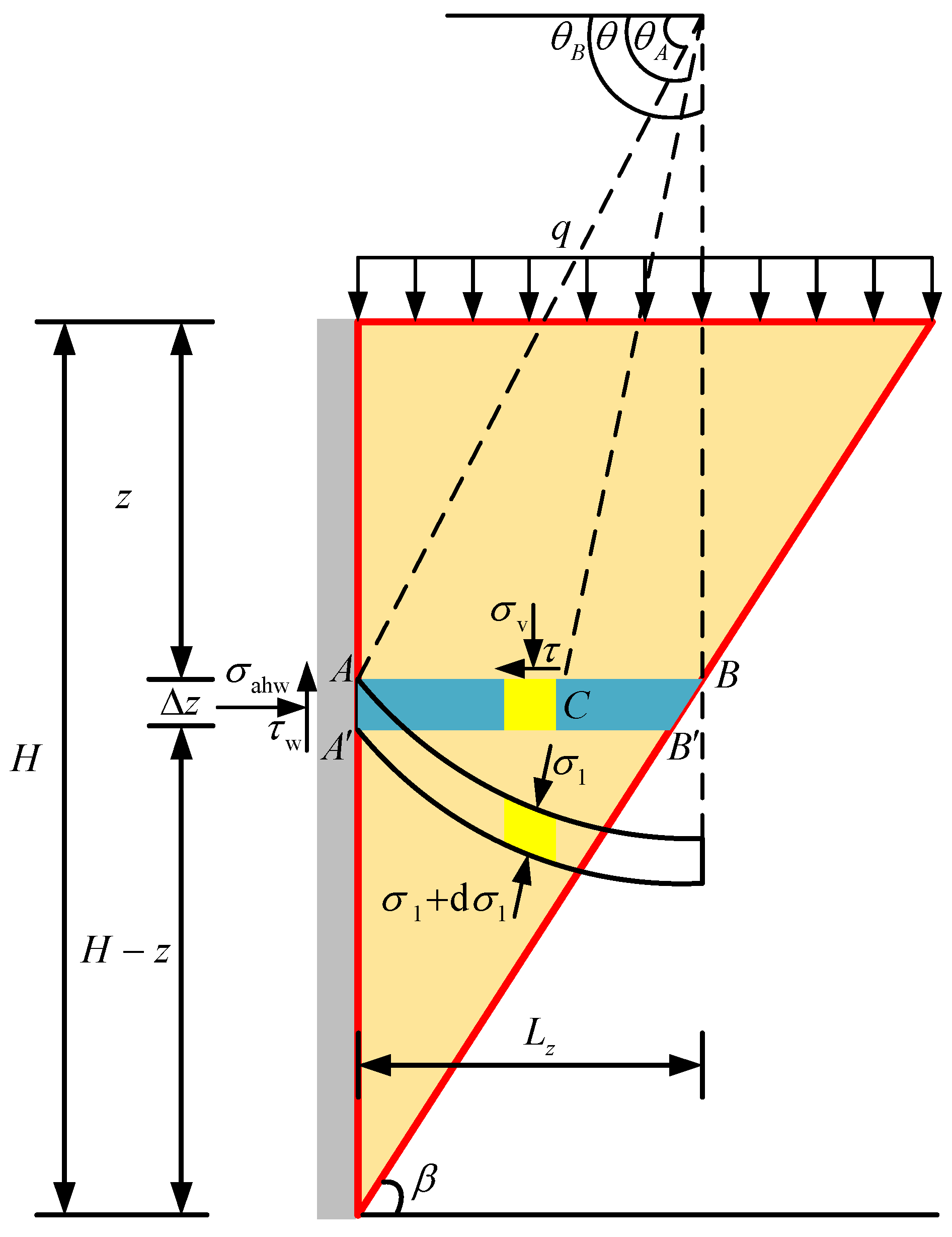
Due to the presence of the vertical arching effect (i.e., the soil arch effect in the vertical plane), the direction of the minor principal stress in the soil is no longer horizontal but deflects to a certain extent. The trace of the minor principal stress within a soil element on the same horizontal layer forms a curve, as shown in Figure 4, which can typically be approximated as an arc [4].

According to the limit equilibrium condition, the deflection angles of the major principal stress at the wall–soil contact surface (point A) and at the sliding surface (point B) are given as follows:

$$\left\{\begin{array}{l}{\theta }_A={\displaystyle \frac{1}{2}}\left[\pi +\delta -\arcsin \left({\displaystyle \frac{\sin \delta }{\sin \phi }}\right)\right]\hfill \\ {\theta }_B={\displaystyle \frac{1}{2}}\left({\displaystyle \frac{\pi }{2}}-\phi \right)+\beta \hfill \end{array}\right.$$

(11)

The stress Mohr circle of the soil behind the shaft wall is translated leftward by ${\sigma }_0$ (i.e., $c\cot \phi$) units, as shown in Figure 5. The stress coordinates of any point in the equivalent coordinate system satisfy the following relationship:

$$\left\{\begin{array}{l}{\sigma }^{\prime }=\sigma +c\cot \phi \hfill \\ {\tau }^{\prime }=\tau \hfill \end{array}\right.$$

(12)

Furthermore, as shown in Figure 4, for the horizontal differential element $AB{B}^{\prime }{A}^{\prime }$ at depth z under the active limit equilibrium state, assuming that the angle between the major principal stress direction at any point C and the horizontal plane is $\theta$, the horizontal stress ${\sigma }_{\mathrm{h}C}^{\prime }$, vertical stress ${\sigma }_{\mathrm{v}C}^{\prime }$, and interlaminar shear stress ${\tau }_C^{\prime }$ at this point are given as follows:

$$\left\{\begin{array}{l}{\sigma }_{\mathrm{h}C}^{\prime }={\sigma }_1^{\prime }\left[{\displaystyle \frac{1+\sin \phi \cos (2\theta )}{1+\sin \phi }}\right]\hfill \\ {\sigma }_{\mathrm{v}C}^{\prime }={\sigma }_1^{\prime }\left[{\displaystyle \frac{1-\sin \phi \cos (2\theta )}{1+\sin \phi }}\right]\hfill \\ {\tau }_C^{\prime }={\sigma }_1^{\prime }\left[{\displaystyle \frac{\sin \phi \sin (2\theta )}{1+\sin \phi }}\right]\hfill \end{array}\right.$$

(13)

By substituting Equation (11) into Equation (13), the horizontal stress (i.e., the horizontal active earth pressure) at point A on the wall–soil contact surface can be obtained as follows:

$${\sigma }_{\mathrm{ahw}}^{\prime }={\sigma }_1^{\prime }\left[{\displaystyle \frac{1+\sin \phi \cos (2{\theta }_A)}{1+\sin \phi }}\right]$$

(14)

Furthermore, the average vertical stress ${\overline{\sigma }}_{\mathrm{v}}^{\prime }$ on the horizontal differential element $AB{B}^{\prime }{A}^{\prime }$ can be expressed as follows:

$${\overline{\sigma }}_{\mathrm{v}}^{\prime }={\displaystyle \frac{{\displaystyle {\int }_{{\theta }_A}^{{\theta }_B}{\sigma }_{\mathrm{v}C}^{\prime }R\sin \theta \mathrm{d}\theta }}{L_z}}={\sigma }_1^{\prime }\left[1-{\displaystyle \frac{2\sin \phi ({\cos }^3{\theta }_A-{\cos }^3{\theta }_B)}{3(1+\sin \phi )(\cos {\theta }_A-\cos {\theta }_B)}}\right]$$

(15)

where $L_z$ is the width of the upper surface of the horizontal differential element $AB{B}^{\prime }{A}^{\prime }$, and $R={\displaystyle \frac{L_z}{\cos {\theta }_A-\cos {\theta }_B}}$;

Similarly, the average shear stress ${\overline{\tau }}^{\prime }$ on the horizontal differential element $AB{B}^{\prime }{A}^{\prime }$ can be obtained as follows:

$${\overline{\tau }}^{\prime }={\displaystyle \frac{{\displaystyle {\int }_{{\theta }_A}^{{\theta }_B}{\tau }_C^{\prime }R\sin \theta \mathrm{d}\theta }}{L_z}}={\sigma }_1^{\prime }\left[{\displaystyle \frac{2\sin \phi ({\sin }^3{\theta }_B-{\sin }^3{\theta }_A)}{3(1+\sin \phi )(\cos {\theta }_A-\cos {\theta }_B)}}\right]$$

(16)

By combining Equations (14) and (15), the lateral active earth pressure coefficient $K_{\mathrm{ahw}}$ can be derived as follows:

$$K_{\mathrm{ahw}}={\displaystyle \frac{{\sigma }_{\mathrm{ahw}}}{{\overline{\sigma }}_{\mathrm{v}}}}={\displaystyle \frac{{\sigma }_{\mathrm{ahw}}^{\prime }-{\sigma }_0}{{\overline{\sigma }}_{\mathrm{v}}^{\prime }-{\sigma }_0}}={\displaystyle \frac{1+\sin \phi \cos (2{\theta }_A)-K_{{\sigma }_0}}{1+\sin \phi \left[1-\frac{2}{3}({\cos }^2{\theta }_A+\cos {\theta }_A\cos {\theta }_B+{\cos }^2{\theta }_B)\right]-K_{{\sigma }_0}}}$$

(17)

where $K_{{\sigma }_0}={\displaystyle \frac{(1+\sin \phi )c}{(\gamma z+q)\tan \phi +c}}$;

Similarly, by combining Equations (15) and (16), the average shear stress coefficient $K_{\tau }$ can be derived as follows:

$$K_{\tau }={\displaystyle \frac{\overline{\tau }}{{\overline{\sigma }}_{\mathrm{v}}}}={\displaystyle \frac{{\overline{\tau }}^{\prime }}{{\overline{\sigma }}_{\mathrm{v}}^{\prime }-{\sigma }_0}}={\displaystyle \frac{2\sin \phi ({\sin }^3{\theta }_B-{\sin }^3{\theta }_A)/3(\cos {\theta }_A-\cos {\theta }_B)}{1+\sin \phi \left[1-\frac{2}{3}({\cos }^2{\theta }_A+\cos {\theta }_A\cos {\theta }_B+{\cos }^2{\theta }_B)\right]-K_{{\sigma }_0}}}$$

(18)

3.2. Circumferential Arching Effect

When the soil behind the shaft wall reaches the active limit state, it is typically accompanied by centripetal displacement, generating a circumferential compression effect that increases the circumferential stress and enhances the stability of the soil. This phenomenon is referred to as the circumferential arching effect. The effect is unevenly distributed within the same horizontal soil layer and gradually weakens with an increase in radial distance, causing the circumferential stress to decrease progressively along the radial direction.

For the horizontal differential element $AB{B}^{\prime }{A}^{\prime }$, the average circumferential stress ${\sigma }_{\mathrm{a}\theta }^{\prime }$ can be obtained using Equation (6) as follows:

$${\sigma }_{a\theta }^{\prime }=\overline{\lambda }{\sigma }_1^{\prime }=\left(1-{\displaystyle \frac{1}{2}}\sin \phi \right){\sigma }_1^{\prime }$$

(19)

Furthermore, by combining Equations (15) and (19), the average circumferential stress coefficient $K_{\theta }$ can be obtained as follows:

$$K_{\theta }={\displaystyle \frac{{\sigma }_{\mathrm{a}\theta }}{{\overline{\sigma }}_{\mathrm{v}}}}={\displaystyle \frac{{\sigma }_{\mathrm{a}\theta }^{\prime }-{\sigma }_0}{{\overline{\sigma }}_{\mathrm{v}}^{\prime }-{\sigma }_0}}={\displaystyle \frac{(1+\sin \phi )(2-\sin \phi )/2-K_{{\sigma }_0}}{1+\sin \phi \left[1-\frac{2}{3}({\cos }^2{\theta }_A+\cos {\theta }_A\cos {\theta }_B+{\cos }^2{\theta }_B)\right]-K_{{\sigma }_0}}}$$

(20)

In summary, considering the influence of the spatial arching effect, the relationships among the horizontal active earth pressure ${\sigma }_{\mathrm{ahw}}^{\prime }$, the average shear stress ${\overline{\tau }}^{\prime }$ between horizontal soil layers, the average circumferential stress ${\sigma }_{\mathrm{a}\theta }^{\prime }$, and the average vertical stress ${\overline{\sigma }}_{\mathrm{v}}^{\prime }$ on the horizontal differential soil element $AB{B}^{\prime }{A}^{\prime }$ have been established.

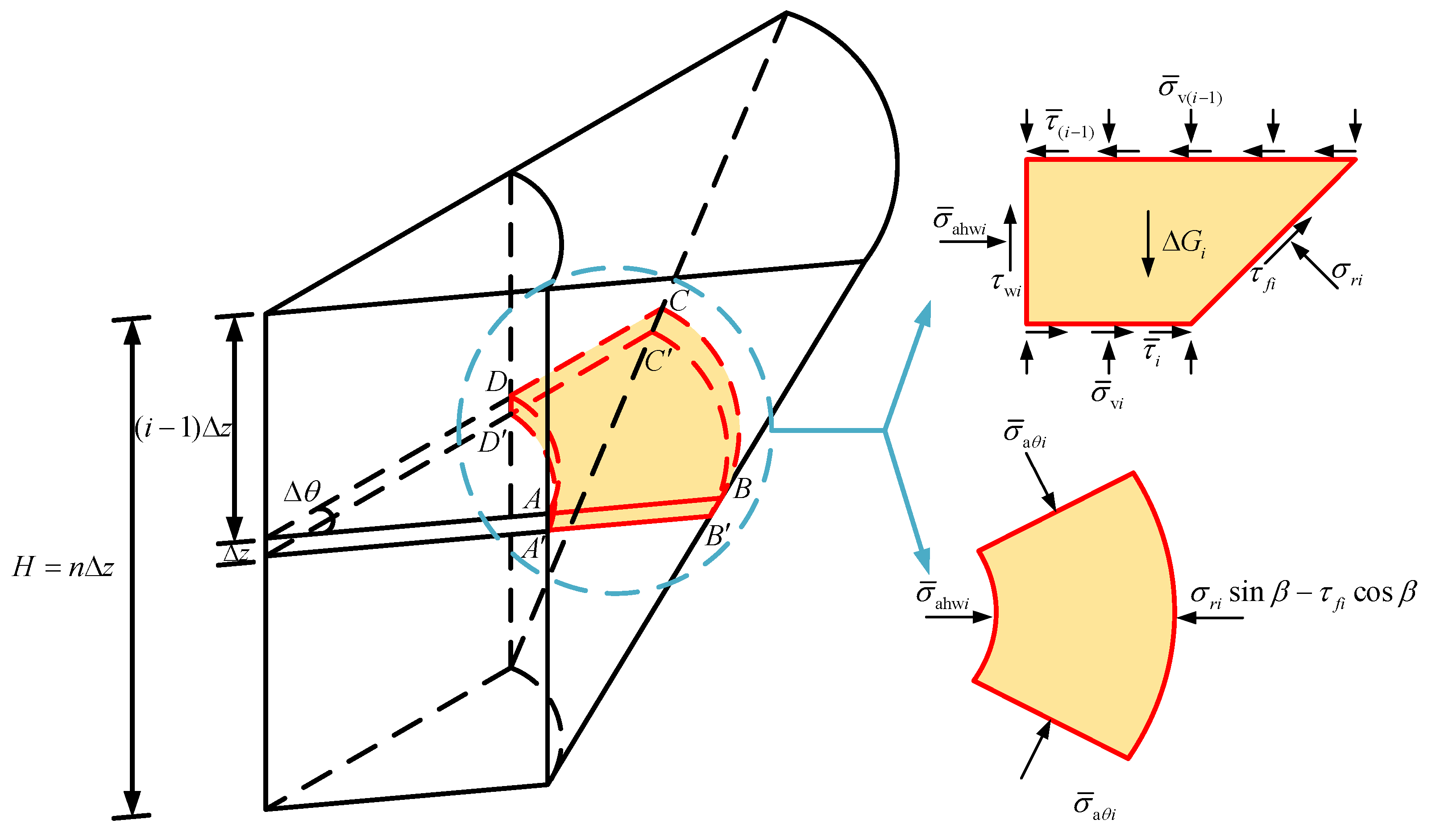
3.3. Numerical Iterative Solution for Active Earth Pressure

This study incorporates interlayer shear stress into the cohesive soil mechanics model. Due to the presence of $\mathrm{d}{\sigma }_0$, it is not possible to obtain an explicit solution for the active earth pressure through integration; therefore, a numerical solution must be employed to derive the active earth pressure. This numerical solution divides the soil into horizontal sections based on the step length $\mathrm{\Delta }z$, as shown in Figure 6. By analyzing the i-th layer of the horizontal differential soil element, the vertical and radial force equilibrium equations are derived as follows (in Figure 6, the shear stress is considered only in the vertical force analysis).

$${\overline{\sigma }}_{\mathrm{v}(i-1)}\cdot S_{ABCD}-{\overline{\sigma }}_{\mathrm{v}i}\cdot S_{A^{\prime }{B}^{\prime }{C}^{\prime }{D}^{\prime }}-{\tau }_{\mathrm{w}i}\cdot S_{AD{D}^{\prime }{A}^{\prime }}-({\sigma }_{ri}\cos \beta +{\tau }_{fi}\sin \beta )\cdot S_{BC{C}^{\prime }{B}^{\prime }}+\mathrm{\Delta }{G}_i=0$$

(21)

$${\overline{\sigma }}_{\mathrm{ahw}i}\cdot S_{AD{D}^{\prime }{A}^{\prime }}-{\overline{\tau }}_{(i-1)}\cdot S_{ABCD}+{\overline{\tau }}_i\cdot S_{A^{\prime }{B}^{\prime }{C}^{\prime }{D}^{\prime }}-({\sigma }_{ri}\sin \beta -{\tau }_{fi}\cos \beta )\cdot S_{BC{C}^{\prime }{B}^{\prime }}+2{\overline{\sigma }}_{\mathrm{a}\theta i}\sin \left({\displaystyle \frac{\mathrm{\Delta }\theta }{2}}\right)\cdot S_{AB{B}^{\prime }{A}^{\prime }}=0$$

(22)

where the action areas $S_{ABCD}$, $S_{A^{\prime }{B}^{\prime }{C}^{\prime }{D}^{\prime }}$, $S_{AD{D}^{\prime }{A}^{\prime }}$, $S_{BC{C}^{\prime }{B}^{\prime }}$, and $S_{AB{B}^{\prime }{A}^{\prime }}$ of each force can be obtained using Equation (23); $\mathrm{\Delta }{G}_i$ is the self-weight of the horizontal differential soil element of the i-th layer, determined by Equation (24). Given the small thickness of the horizontal differential soil element, it is assumed that within the thickness $\mathrm{\Delta }z$, the horizontal stress at the wall–soil contact surface and the circumferential stress of the soil element are approximately linearly distributed, which can be calculated using Equation (25). The remaining parameters can be determined using Equation (26), based on the stress relationships derived from the active limit equilibrium condition and the spatial arching effect.

$$\left\{\begin{array}{l}{S}_{ABCD}=\left[{\displaystyle \frac{H-(i-1)\mathrm{\Delta }z}{\tan \beta }}\right]\left[r_0+{\displaystyle \frac{H-(i-1)\mathrm{\Delta }z}{2\tan \beta }}\right]\mathrm{\Delta }\theta \hfill \\ S_{A^{\prime }{B}^{\prime }{C}^{\prime }{D}^{\prime }}=\left({\displaystyle \frac{H-i\mathrm{\Delta }z}{\tan \beta }}\right)\left(r_0+{\displaystyle \frac{H-i\mathrm{\Delta }z}{2\tan \beta }}\right)\mathrm{\Delta }\theta \hfill \\ S_{AD{D}^{\prime }{A}^{\prime }}=r_0\mathrm{\Delta }\theta \mathrm{\Delta }z\hfill \\ S_{BC{C}^{\prime }{B}^{\prime }}=\left[r_0+{\displaystyle \frac{H-(i-1)\mathrm{\Delta }z}{\tan \beta }}\right]{\displaystyle \frac{\mathrm{\Delta }\theta \mathrm{\Delta }z}{\sin \beta }} \hfill \\ S_{AB{B}^{\prime }{A}^{\prime }}=S_{CD{D}^{\prime }{C}^{\prime }}=\left[{\displaystyle \frac{2H-(2i-1)\mathrm{\Delta }z}{2\tan \beta }}\right]\mathrm{\Delta }z\hfill \end{array}\right.$$

(23)

$$\mathrm{\Delta }{G}_i=\gamma \left({\displaystyle \frac{S_{ABCD}+S_{A^{\prime }{B}^{\prime }{C}^{\prime }{D}^{\prime }}}{2}}\right)\mathrm{\Delta }z$$

(24)

$$\left\{\begin{array}{l}{\overline{\sigma }}_{\mathrm{ahw}i}={\displaystyle \frac{\left[K_{\mathrm{ahw}(i-1)}{\overline{\sigma }}_{\mathrm{v}(i-1)}+K_{\mathrm{ahw}i}{\overline{\sigma }}_{\mathrm{v}i}\right]}{2}}\hfill \\ {\overline{\sigma }}_{\mathrm{a}\theta i}={\displaystyle \frac{\left[K_{\theta (i-1)}{\overline{\sigma }}_{\mathrm{v}(i-1)}+K_{\theta i}{\overline{\sigma }}_{\mathrm{v}i}\right]}{2}}\hfill \end{array}\right.$$

(25)

$$\left\{\begin{array}{l}{\overline{\tau }}_i=K_{\tau i}{\overline{\sigma }}_{\mathrm{v}i}\hfill \\ {\tau }_{\mathrm{w}i}={\overline{\sigma }}_{\mathrm{ahw}i}\tan \delta +c_{\mathrm{w}}\hfill \\ {\tau }_{fi}={\sigma }_{ri}\tan \phi +c\hfill \end{array}\right.$$

(26)

By combining Equations (21)–(26), the iterative formula for a can be established:

$${\overline{\sigma }}_{\mathrm{v}i}={\displaystyle \frac{{\alpha }_{\sigma (i-1)}{\overline{\sigma }}_{\mathrm{v}(i-1)}-{\alpha }_{c}c-{\alpha }_{c_{\mathrm{w}}}{c}_{\mathrm{w}}+\mathrm{\Delta }{G}_i}{{\alpha }_{{\sigma }_i}}}$$

(27)

where

• ${\alpha }_{\sigma (i-1)}=\left[1+K{K}_{\tau (i-1)}\right]S_{ABCD}-\frac{1}{2}{K}_{\mathrm{ahw}(i-1)}(K+\tan \delta )S_{AD{D}^{\prime }{A}^{\prime }}-\frac{1}{2}K{K}_{\theta (i-1)}\mathrm{\Delta }\theta S_{AB{B}^{\prime }{A}^{\prime }}$;
• ${\alpha }_{\sigma i}=(1+K{K}_{\tau i})S_{A^{\prime }{B}^{\prime }{C}^{\prime }{D}^{\prime }}+\frac{1}{2}{K}_{\mathrm{ahw}i}(K+\tan \delta )S_{AD{D}^{\prime }{A}^{\prime }}+\frac{1}{2}K{K}_{\theta i}\mathrm{\Delta }\theta S_{AB{B}^{\prime }{A}^{\prime }}$;
• ${\alpha }_c=(\sin \beta +K\cos \beta )S_{BC{C}^{\prime }{B}^{\prime }}$; ${\alpha }_{c_{\mathrm{w}}}=S_{AD{D}^{\prime }{A}^{\prime }}$;$K={\displaystyle \frac{1+\tan \phi \tan \beta }{\tan \beta -\tan \phi }}$;

The active earth pressure of the horizontal differential soil elements below the critical depth and above the critical stress is summed to obtain the resultant active earth pressure:

$$P_a={\displaystyle \sum _{i=i_a}^{i_b}\sqrt{{(K_{\mathrm{ahw}i}{\overline{\sigma }}_{\mathrm{v}i})}^2+{(K_{\mathrm{ahw}i}{\overline{\sigma }}_{\mathrm{v}i}\tan \delta +c_{\mathrm{w}})}^2}}\mathrm{\Delta }z$$

(28)

where $i_a$ is the i value at the critical depth, which can be determined using Equation (29); $i_b$ is the i value at the critical stress at the bottom of the shaft; that is, the i value corresponding to the point when Equation (27) is iterated to 0.

$$i_a={\displaystyle \frac{1}{\gamma \mathrm{\Delta }z}}\left\{{\displaystyle \frac{c\cot \phi \left[1-\cos (2{\theta }_A)\right]}{1+\sin \phi \cos (2{\theta }_A)}}-q\right\}$$

(29)

The total overturning moment caused by the active earth pressure on the wall heel is given by:

$$M_a={\displaystyle \sum _{i=i_a}^{i_b}{K}_{\mathrm{ahw}i}{\overline{\sigma }}_{\mathrm{v}i}}\mathrm{\Delta }z\left[H-\left({\displaystyle \frac{2i-1}{2}}\right)\mathrm{\Delta }z\right]$$

(30)

From Equation (30), the position of the active earth pressure resultant force can be finally obtained as:

$$h_a={\displaystyle \frac{M_a}{{\displaystyle \sum _{i=i_a}^{i_b}{K}_{\mathrm{ahw}i}{\overline{\sigma }}_{\mathrm{v}i}\mathrm{\Delta }z}}}+(H-i_b\mathrm{\Delta }z)$$

(31)

3.4. Validation and Comparison with Other Theoretical and Experimental Results

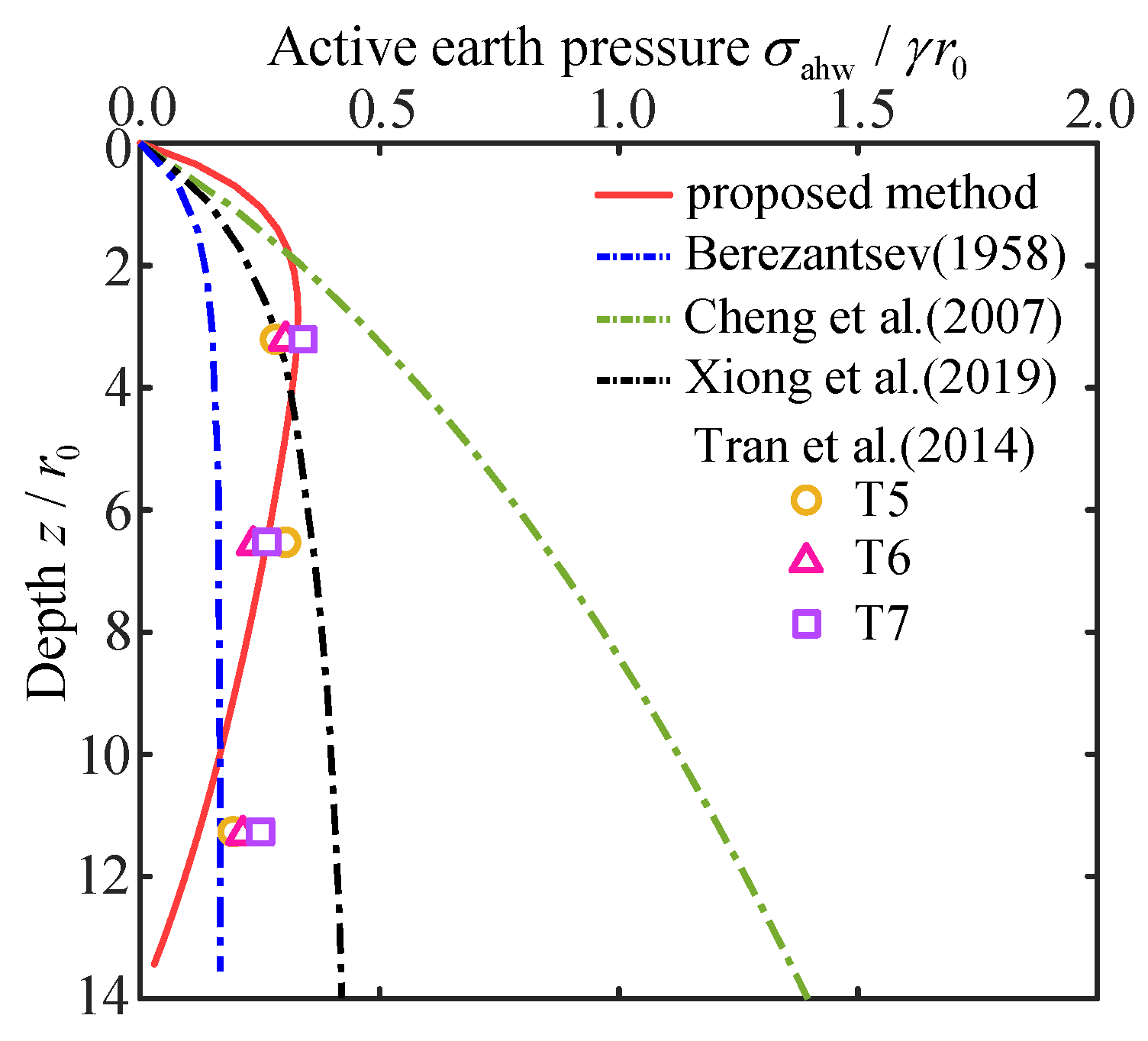
Tran et al. [34] employed a circular shaft model with a uniformly decreasing diameter to investigate the distribution of active earth pressure on the shaft wall. The relevant parameters of the model test are: $\phi =41°,\delta =0, c=0,$ $\gamma =14.7 \mathrm{kN}/{\mathrm{m}}^3, r_0/H=0.075$. Figure 7 compares the calculation results obtained in this study with the experimental results of Tran et al. [34], and further compares and analyzes them alongside the theoretical predictions of Berezantsev [16], Cheng et al. [19], and Xiong et al. [29].

As shown in Figure 7, the calculated values from this study and those of Xiong et al. [29] are generally consistent with the model test results. It is noteworthy that this study incorporates the spatial arching effect of the soil in the calculation, which allows for a more accurate representation of the trend where the soil pressure intensity first increases and then decreases with depth. In contrast, the calculation results of Berezantsev [16] and Cheng et al. [19] show significant deviations from the experimental values. The primary reason is that both studies assume the circumferential stress coefficient $\lambda$ to be constant (1 and K₀, respectively), neglecting the fact that the circumferential stress continuously varies with position. By comparison, this study accounts for the variation of the circumferential stress coefficient $\lambda$ along the radial coordinate, resulting in calculated values that are closer to the experimental results and thereby verifying the rationality and effectiveness of the proposed calculation method.

To further analyze the influence of the radius-to-height ratio and wall–soil friction angle on the distribution of active earth pressure intensity, Figure 8 presents the distribution curves of active earth pressure intensity under different radius-to-height ratios and wall–soil friction angles. Additionally, to investigate the role of the interlayer shear effect of the soil, the calculation results of this study are compared with the values reported by Lu et al. [21]. For ease of analysis, both the horizontal and vertical axes in the figure are normalized.

As shown in the figure, the active earth pressure intensity obtained in this study exhibits a curved distribution. The smaller the radius-to-height ratio and the larger the wall–soil friction angle, the more pronounced the influence of the soil arching effect on the distribution of active earth pressure intensity, and the more evident the curved distribution characteristics. In addition, when the radius-to-height ratio is less than 1, the calculated active earth pressure intensity in the middle and lower portions of the shaft is significantly lower than the theoretical value predicted by Rankine’s earth pressure theory. As the radius-to-height ratio increases, the circumferential arching effect gradually weakens, and the active earth pressure intensity at the same depth progressively increases; however, the rate of increase gradually diminishes.

Further comparative analysis of the calculation results of Lu et al. [21] reveals that the shear stress between soil layers has a substantial impact on the distribution of active earth pressure along the depth direction. This effect is primarily reflected in the reduction of active earth pressure in the middle and upper portions of the shaft and the increase of active earth pressure at the shaft bottom. Moreover, the larger the radius-to-height ratio and the larger the wall–soil friction angle, the more pronounced the influence of interlayer shear on the active earth pressure distribution.

However, it should be noted that the assumption of a linear sliding surface extending to the bottom of the shaft results in a sudden drop in the calculated earth pressure to 0 at the base. As this discontinuity is distinctly localized and has a minimal effect on the overall distribution, a practical adjustment can be adopted in engineering applications by extrapolating the earth pressure value computed at 95% of the shaft depth to the bottom 5%.

4. Analysis of Internal Forces and Deformations in Circular Shaft Structures

4.1. Model Formulation and Assumptions

The circular shaft is shown in Figure 9a. The inner and outer diameters of the shaft support structure are denoted as r and R, respectively. It is subjected to internal pressure p₁ and external pressure p₂. To determine the distribution of internal forces and deformations, the following assumptions are made:

(1) Cracking of the structure is ignored, and the stress and deformation of the supporting structure are assumed to be elastic.

(2) Three-dimensional effects are ignored, and the support structure is modeled as a thick-walled cylinder.

Under the above assumptions, the stress and deformation problem in the shaft support structure is analyzed in the polar coordinate system using elasticity theory. The analytical model is shown in Figure 9b, with boundary conditions satisfying Equation (32).

$$\left\{\begin{array}{c}{\sigma }_{\rho }{|}_{\rho =r}=-q_1\hfill \\ {\sigma }_{\rho }{|}_{\rho =R}=-q_2\hfill \\ {\tau }_{\rho \phi }{|}_{\rho =r}=0\hfill \\ {\tau }_{\rho \phi }{|}_{\rho =R}=0\hfill \end{array}\right.$$

(32)

where σ_ρ is the radial stress; σ_φ is the circumferential stress; τ_ρφ is the shear stress; q₁ and q₂ are the internal and external pressures, respectively.

4.2. Analytical for Internal Forces and Deformations

The problem is treated as axisymmetric, where the stress and strain components depend only on ρ, not φ, and the shear stress τ_ρφ is zero.

Since Equation (32) defines the stress boundary conditions, the solution can be obtained using the stress function method. The stress function is a scalar function of ρ and is expressed as Equation (33):

$$\mathrm{\Phi }=\mathrm{\Phi }\left(\rho \right)$$

(33)

where Φ is the stress function, while ρ and φ represent the radial and circumferential coordinates in the polar coordinate system, respectively.

In elasticity theory, the stress function in Equation (33) must satisfy the compatibility equation, given in Equation (34), and the general solution is given by Equation (35):

$${\mathrm{\Delta }}^2\mathrm{\Phi }=0$$

(34)

$$\mathrm{\Phi }=A\ln \rho +B{\rho }^2\ln \rho +C{\rho }^2+D$$

(35)

where Δ is the Laplace operator; A, B, C, and D are constants to be determined.

The general stress solution is derived from Equation (35) and given in Equation (36):

$$\left\{\begin{array}{l}{\sigma }_{\rho }={\displaystyle \frac{A}{{\rho }^2}}+B\left(1+2\ln \rho \right)+2C\\ {\sigma }_{\phi }=-{\displaystyle \frac{A}{{\rho }^2}}+B\left(3+2\ln \rho \right)+2C\\ {\tau }_{\rho \phi }=0\end{array}\right.$$

(36)

Substituting Equation (36) into the physical equation and combining it with the geometric equation yields the deformation solution to this problem, as shown in Equation (37):

$$\left\{\begin{array}{l}{u}_{\rho }={\displaystyle \frac{1}{E}}\left[-\left(1+v\right){\displaystyle \frac{A}{\rho }}+2\left(1-v\right)B\rho \left(\ln \rho -1\right)+\left(1-3v\right)B\rho +2\left(1-v\right)C\rho \right]\\ u_{\phi }={\displaystyle \frac{4B\rho \phi }{E}}\end{array}\right.$$

(37)

where E is the elastic modulus; v is the Poisson’s ratio; u_ρ is the radial deformation; u_φ is the radial deformation.

4.3. Analysis of Internal Forces and Deformations

By combining Equations (32) and (36) together with the single-valued condition for circumferential displacement, the parameters are determined as shown in Equation (38):

$$\left\{\begin{array}{l}A={\displaystyle \frac{r^2{R}^2\left(p_2-p_1\right)}{R^2-r^2}}\\ B=0\\ C={\displaystyle \frac{p_1{r}^2-p_2{R}^2}{2\left(R^2-r^2\right)}}\end{array}\right.$$

(38)

Combining Equations (36) and (38), the stress distribution is obtained as Equation (39):

$$\left\{\begin{array}{l}{\sigma }_{\rho }={\displaystyle \frac{r^2{R}^2\left(p_2-p_1\right)}{R^2-r^2}}{\displaystyle \frac{1}{{\rho }^2}}+{\displaystyle \frac{p_1{r}^2-p_2{R}^2}{R^2-r^2}}\\ {\sigma }_{\phi }=-{\displaystyle \frac{r^2{R}^2\left(p_2-p_1\right)}{R^2-r^2}}{\displaystyle \frac{1}{{\rho }^2}}+{\displaystyle \frac{p_1{r}^2-p_2{R}^2}{R^2-r^2}}\\ {\tau }_{\rho \phi }=0\end{array}\right.$$

(39)

By substituting Equation (38) into Equation (37), the deformation distribution is given by Equation (40):

$$\left\{\begin{array}{l}{u}_{\rho }={\displaystyle \frac{1}{E}}\left[-{\displaystyle \frac{r^2{R}^2\left(p_2-p_1\right)}{R^2-r^2}}{\displaystyle \frac{1+v}{\rho }}+{\displaystyle \frac{p_1{r}^2-p_2{R}^2}{R^2-r^2}}\left(1-v\right)\rho \right]\\ u_{\phi }=0\end{array}\right.$$

(40)

5. A Case Study

To further validate the proposed calculation method, this study conducted a comparative analysis between the computed results and the field monitoring data.

5.1. Project Overview

The Mingyuan Forest Urban Green Underground Smart Garage Project is located at the southeast corner of Guangyan Road and Yonghe Road in Jingan District, Shanghai. The project comprised two circular shafts with an inner diameter of 21.0 m, constructed by mechanical excavation. In mechanical shaft construction, the segmental lining was installed by a top-down, ring-by-ring assembly synchronized with the shaft’s progressive sinking. The first ring was pre-assembled on the ground or in a shallow shaft. As excavation proceeded in stages and the shaft subsided, subsequent rings were installed sequentially within the sinking space. Each ring was bolted and sealed to ensure structural integrity and watertightness. Each shaft support structure consisted of three components: a 2.0 m thick cast-in-place bladed footing at the base, 22 rings of precast segmental linings totaling 44.0 m in height, and a 4.2 m high cast-in-place top section. For convenience in the following analysis, the blade foot was designated as Ring 0, and the precast segments were consecutively numbered from Ring 1 to Ring 22 in ascending order from bottom to top. The shaft excavation diameter was 23.0 m, with a segment thickness of 1.0 m. Each ring comprised 10 segments. The total excavation depth was approximately 50.2 m. The relevant geological parameters are listed in

Table 1. Geological parameters.

Soil	Thickness/(m)	Unit Weight/(kN·m−3)	Internal Friction Angle/(°)	Cohesion/(kPa)
Clayey silt	3.5	18.7	25	10
Soft plastic silty clay	10.3	17.8	14	14
Plastic silty clay	6.1	18.1	16	17
Hard plastic silty clay	3.2	19.9	18	18
Silty clay interbedded with sandy silt	6.6	19	19	24
Hard plastic silty clay	16.3	18.3	18	19
Silty clay interbedded with sandy silt	7.3	18.5	23	14

Since the physical and mechanical parameters of each soil layer varied slightly, the subsequent earth pressure analysis used the weighted average method based on soil layer thickness, treating the multi-layer soil as a single homogeneous layer.

.

The circular shaft case study aligns well with the calculation model proposed herein, and the comparative validation based on this case is both appropriate and robust. In addition, to verify the reliability of the analytical results, vibrating wire earth pressure gauges and steel reinforcement bar axial force gauges were installed to monitor the earth pressure on the Ring 3 and Ring 6 segments, as well as the axial forces in the inner and outer reinforcement bars, respectively. The locations of the monitoring points are shown in Figure 10.

To facilitate subsequent analysis, based on the on-site construction plan and the stress characteristics of the support structure, the shaft construction process was divided into three stages.

Stage I: Excavation to the bottom under the condition that the outer wall was in contact with slurry and the inner wall was in contact with silty water. The unit weight of silty water on the inner wall was 12.5 kN/m³, and the unit weight of slurry on the outer wall was 11.0 kN/m³.

Stage II: Replacement of the slurry on the outer wall with plain concrete.

Stage III: Extraction of water from inside the shaft.

Since both the inner and outer sides of the segments were surrounded by fluid in Stage I, and therefore not subjected to earth pressure, the earth pressure analysis was conducted only for Stages II and III.

5.2. Analysis of the Internal and External Pressures on the Segment

Figure 11 compares the calculated active earth pressure, the theoretical value from Rankine’s earth pressure theory, and the monitoring data from Shaft No. 2 of the Jingan Garage. As shown in the figure, the theoretical values obtained from the method proposed in this study are in good agreement with the measured results. It can serve as a theoretical basis for the optimal design of circular shaft wall structures.

This is primarily attributed to the inclusion of soil arching effects in both the vertical and horizontal planes in the calculation. In particular, the consideration of the ring arching effect in the horizontal plane greatly improved the stability of the surrounding soil, thereby reducing the active earth pressure acting on the shaft wall. These results further validate the rationality and accuracy of the proposed calculation method.

For clarity and efficiency, Rings 3, 6, 10, 14, 18, and 22 were selected for analysis.

Table 2. Internal and external pressures on the segment at Stage I.

Ring	Depth/(m)	p1/kPa	p2/kPa	p2 Monitored/(kPa)
22	6	−72.00	−66.00	-
18	14	−168.00	−154.00	-
14	22	−264.00	−242.00	-
10	30	−360.00	−330.00	-
6	38	−456.00	−418.00	−390.00
3	44	−528.00	−484.00	−451.96

,

Table 3. Internal and external pressures on the segment at Stage II.

Ring	Depth/(m)	p1/kPa	p2 Proposed Method/kPa	p2 Rankine/kPa	p2 Monitored/(kPa)
22	6	−72.00	−45.31	−39.68	-
18	14	−168.00	−136.36	−127.38	-
14	22	−264.00	−179.85	−213.48	-
10	30	−360.00	−271.28	−300.28	-
6	38	−456.00	−318.97	−387.08	−272.65
3	44	−528.00	−310.08	−452.18	−339.67

and

Table 4. Internal and external pressures on the segment at Stage III.

Ring	Depth/(m)	p1/kPa	p2 Proposed Method/kPa	p2 Rankine/kPa	p2 Monitored/(kPa)
22	6	0.00	−38.65	−33.16	-
18	14	0.00	−129.92	−108.76	-
14	22	0.00	−179.85	−184.36	-
10	30	0.00	−217.28	−259.96	-
6	38	0.00	−237.32	−335.56	−190.33
3	44	0.00	−210.36	−392.26	−175.47

show the calculated internal and external pressures on the segments during the three construction stages.

5.3. Analysis of the Internal Forces and External Deformations

Figure 12 shows the contour plots of the analytical results for the radial internal forces, circumferential internal forces, and radial deformation of the Ring 3 segment during Stage I. As shown in the figure, the internal forces and deformations exhibited a clear symmetrical pattern, which is consistent with engineering practice.

Based on the assumptions of the plane section, linear elasticity, and uncracked concrete, the axial force in the steel bars and the circumferential stress at the section center, as obtained from monitoring, can be calculated using Equation (41):

$${\sigma }_{\phi }^{\prime }={\displaystyle \frac{N_{s1}+N_{s2}}{2E_s}}{E}_c$$

(41)

where σ′_φ is the circumferential internal stress; N_s1 and N_s2 are the monitored axial forces in the steel bars on the outer and inner sides of the segment, respectively; E_s is the elastic modulus of the steel bars; and E_c is the elastic modulus of the reinforced concrete.

Figure 13 presents a comparison between the theoretical calculations and the monitored values of the annular internal forces for Rings 3 and 6. As shown in the figure, the relative error between the results obtained from earth pressure theory and the measured values was within 10%, with a correlation coefficient of 0.98, indicating a strong correlation between the analytical and monitored values. The error falls within a reasonable range, verifying the reliability of the proposed analysis.

Figure 14 shows the analysis results of internal forces. As observed from Figure 13 and Figure 14, the internal forces were positively correlated with the burial depth. When the internal pressure exceeded the external pressure, the maximum radial stress occurred at the inner arc surface, while the maximum radial deformation and circumferential stress occurred at the outer arc surface. Conversely, when the external pressure was greater than the internal pressure, the pattern was reversed. A large pressure difference between the inside and outside can result in excessive forces on the segment, while excessive internal pressure may cause the segment to undergo tension. In practical engineering, it is important to avoid both large pressure differences and excessive internal pressure.

Figure 15 presents the internal forces and deformation along the depth direction, where the solid line corresponds to the outcomes derived from the calculation method proposed herein, while the dotted line represents the results based on the Rankine earth pressure theory.

① During the first stage, the internal forces and deformations of the segment increased approximately linearly with burial depth, consistent with the linear growth of soil and fluid pressures acting on the segment at this stage. In contrast, segments in the second and third stages exhibited distinct nonlinear variations in force and deformation along the depth. This discrepancy primarily resulted from the fact that, in the first stage, the segment’s inner and outer surfaces were subjected to silt and slurry pressures respectively, both varying linearly with depth. However, the earth pressure model developed in this study incorporates the soil arching effect, producing a nonlinear earth pressure distribution, which in turn induces nonlinear responses in segment forces and deformations.

② In the second stage, the segment experienced maximum annular internal force and radial deformation at a burial depth near 38.0 m, while in the third stage, these maxima occurred closer to 23.0 m depth. This phenomenon was mainly driven by the evolving differential pressure across the segment. As construction advanced and surrounding ground conditions changed, the distribution of pressure difference was altered, leading to stage-dependent shifts in the locations of peak force and deformation. These results reveal the complex temporal and spatial evolution of segment stress states during construction, providing valuable guidance for the rational design of segment structures and effective construction control strategies.

6. Conclusions

In this study, the stress and deformation behavior of circular shafts was analyzed by explicitly incorporating the radial distribution of circumferential stress induced by the spatial arching effect. An analytical expression for the inclination angle of the sliding surface under active limit conditions was derived based on the global force equilibrium of the sliding soil. A novel method for calculating the active earth pressure on circular shafts was proposed, which accounts for both the spatial arching effect and interlayer shear interactions. The validity of the proposed approach was confirmed through comparisons with theoretical solutions, model test results, and field measurements. Furthermore, an elastic mechanics-based model was developed to evaluate the stress and deformation response of pipe segments during mechanical shaft excavation. The main conclusions are summarized as follows:

(1) Under active limit conditions, the inclination angle of the sliding surface behind the circular shaft wall is generally larger than that of the Coulomb sliding surface. As the radius-to-height ratio increases, the spatial arching effect—particularly the circumferential arching effect—gradually diminishes, leading to a decrease in the sliding surface angle that asymptotically approaches the theoretical prediction. Additionally, higher soil cohesion increases the shear stress required to satisfy limit equilibrium, thereby resulting in a greater sliding surface angle. This effect is more pronounced in soils with lower internal friction angles.

(2) The active earth pressure of circular shafts is significantly influenced by the radius-to-height ratio and interlayer shear stress: a smaller radius-to-height ratio enhances the circumferential arching effect, improving soil stability and reducing active earth pressure, while a larger diameter-to-height ratio amplifies the impact of interlayer shear stress on the pressure distribution. By accounting for the radial variation of the circumferential stress coefficient and the spatial arching effect, the proposed calculation method shows good agreement with model test results and effectively captures the depth-dependent variation of active earth pressure under the translation mode.

(3) The stress and deformation behavior of the shaft structure is fundamentally governed by the combined action of internal and external water and soil pressures. Owing to the spatial arching effect of the surrounding soil mass, the distribution of stresses and deformations in Stages II and III demonstrates a distinct nonlinear variation with depth. The analytical predictions show excellent agreement with the measured data, thereby confirming the validity and reliability of the proposed earth pressure calculation framework and the structural stress–deformation analysis approach developed in this study.

(4) The stresses experienced by the shaft structure are strongly governed by the pressure differential between its inner and outer sides. An excessive pressure differential can induce elevated structural stresses, while overly high internal pressures may subject the structure to significant tensile forces. Therefore, in practical engineering applications, it is crucial to carefully control both the pressure differential and the internal pressure to ensure the structural integrity and long-term safety of the shaft system.

In summary, the proposed calculation framework provides a theoretical basis for the optimization and safety evaluation of circular shaft wall structures under translational mode conditions. Moreover, the underlying concepts offer potential reference value for investigating displacement behavior under rotational failure modes, with prospects for broader application and further development.

References

1. Tsagareli, Z.V. Experimental investigation of the pressure of a loose medium on retaining walls with a vertical back face and horizontal backfill surface. Soil Mech. Found. Eng. 1965, 2, 197–200. [Google Scholar] [CrossRef]
2. Neal, T.S.; Hagerty, D.J. Earth pressures in confined cohesionless backfill against tall rigid walls-a case history. Can. Geotech. J. 2011, 48, 1188–1197. [Google Scholar]
3. Tobar, T.; Meguid, M.A. Comparative evaluation of methods to determine the earth pressure distribution on cylindrical shafts: A review. Tunn. Undergr. Space Technol. 2010, 25, 188–197. [Google Scholar] [CrossRef]
4. Handy, R.L. The arch in soil arching. J. Geotech. Eng. 1985, 111, 302–318. [Google Scholar] [CrossRef]
5. Paik, K.H.; Salgado, R. Estimation of active earth pressure against rigid retaining walls considering arching effects. Géotechnique 2003, 53, 643–653. [Google Scholar] [CrossRef]
6. Goel, S.; Patra, N.R. Effect of arching on active earth pressure for rigid retaining walls considering translation mode. Int. J. Geomech. 2008, 8, 123–133. [Google Scholar] [CrossRef]
7. Liu, H.; Kong, D.; Gan, W.; Wang, B. Seismic active earth pressure of limited backfill with curved slip surface considering intermediate principal stress. Appl. Sci. 2021, 12, 169. [Google Scholar] [CrossRef]
8. Wang, X.; Dang, F.; Cao, X.; Zhang, L.; Gao, J.; Xue, H. Solution for Active and Passive Earth Pressure on Rigid Retaining Walls with Narrow Backfill. Appl. Sci. 2025, 15, 1750. [Google Scholar] [CrossRef]
9. Zhang, Z.L.; Zhu, J.Q.; Yang, X.L. Three-dimensional active earth pressures for unsaturated backfills with cracks considering steady seepage. Int. J. Geomech. 2023, 23, 04022270. [Google Scholar] [CrossRef]
10. He, Z.; Liu, Z.; Liu, X.; Bian, H. Improved method for determining active earth pressure considering arching effect and actual slip surface. J. Cent. South Univ. 2020, 27, 2032–2042. [Google Scholar] [CrossRef]
11. Khosravi, M.H.; Kargar, A.R.; Amini, M. Active earth pressures for non-planar to planar slip surfaces considering soil arching. Int. J. Geotech. Eng. 2020, 14, 730–739. [Google Scholar] [CrossRef]
12. Yu, P.; Liu, Y. Analysis of active earth pressure behind rigid retaining walls considering curved slip surface. Geotech. Geol. Eng. 2024, 42, 251–270. [Google Scholar] [CrossRef]
13. Terzaghi, K. Theoretical Soil Mechanics; John Wiley and Sons: New York, NY, USA, 1943; pp. 165–182. [Google Scholar]
14. Ma, Y.M. Theory and practice of ground pressure on shaft due to thick overburden. J. China Univ. Min. Technol. 1979, 1, 48–72. [Google Scholar]
15. Fujii, T.; Hagiwara, T.; Kusakabe, O. Active failure mechanism of a deep circular shaft in dry sand. In Proceedings of the Geotechnical Aspects of Underground Construction in Soft Ground, University of London, London, UK, 15 April 1996; pp. 137–142. [Google Scholar]
16. Berezantzev, V.G. Earth pressure on the cylindrical retaining walls. In Proceedings of the Brussels Conference on Earth Pressure Problems, II, Brussels, Belgium, 20 September 1958. [Google Scholar]
17. Prater, E.G. An examination of some theories of earth pressure on shaft linings. Can. Geotech. J. 1977, 14, 91–106. [Google Scholar] [CrossRef]
18. Cui, G.X. Loading of shaft lining for deep alluvium. Chin. J. Geotech. Eng. 2003, 25, 294–298. [Google Scholar]
19. Cheng, Y.M.; Hu, Y.Y.; Wei, W.B. General axisymmetric active earth pressure by method of characteristics—Theory and numerical formulation. Int. J. Geomech. 2007, 7, 1–15. [Google Scholar] [CrossRef]
20. Chen, G.Z.; Zhou, G.Q. Active earth pressure on cylindrical wall with consideration of soil arching effects. J. Jiangsu Univ. Nat. Sci. Ed. 2015, 36, 108–113. [Google Scholar]
21. Lu, K.L.; Zhou, G.G.; Yang, Y. Active earth pressure on a cylindrical retaining wall with considering the spatial arching effect. Arab. J. Geosci. 2022, 15, 1274. [Google Scholar] [CrossRef]
22. Zhang, J.; Li, M.; Ke, L.; Yi, J. Distributions of lateral earth pressure behind rock-socketed circular diaphragm walls considering radial deflection. Comput. Geotech. 2022, 143, 104604. [Google Scholar] [CrossRef]
23. Zhang, J.; Li, M.; Yi, J.; Wu, D.; Chai, X. Analytical Solution for Radial Displacement–Dependent Earth Pressure Acting on Underwater Rock-Socketed Circular Diaphragm Walls. Int. J. Geomech. 2024, 24, 4024083. [Google Scholar] [CrossRef]
24. Jia, S.; Zhou, G.; Qin, T.; Mei, Y.; Li, J.; Lu, K. Calculation of Active Earth Pressure on a Circular Retaining Wall Based on Energy Method. In Proceedings of Conference on Sustainable Traffic and Transportation Engineering; Springer Nature: Singapore, 2023. [Google Scholar]
25. Pedro, A.M. A Methodology to Evaluate the Horizontal Earth Pressure Acting on Circular Shafts Based on Its Lateral Displacements. Geotechnics 2024, 4, 952–965. [Google Scholar] [CrossRef]
26. Liu, F.Q.; Wang, J.H. A generalized slip line solution to the active earth pressure on circular retaining walls. Comput. Geotech. 2008, 35, 155–164. [Google Scholar] [CrossRef]
27. Liu, F.Q.; Wang, J.H.; Zhang, L.L. Analytical solution of general axisymmetric active earth pressure. Int. J. Numer. Anal. Methods Geomech. 2009, 33, 551–565. [Google Scholar] [CrossRef]
28. Chen, G.Z.; Zhou, G.Q. Discrete element analysis of active earth pressure against the cylindrical wall. Chin. J. Undergr. Space Eng. 2013, 9, 1848–1852. [Google Scholar]
29. Xiong, G.J.; Wang, J.H.; Chen, J.J. Theory and practical calculation method for axisymmetric active earth pressure based on the characteristics method considering the compatibility condition. Appl. Math. Model. 2019, 68, 563–582. [Google Scholar] [CrossRef]
30. Xiong, G.J.; Wang, J.H.; Chen, J.J. Analytical solution for axisymmetric active earth pressure based on the characteristics method considering orthoradial geometric condition. Int. J. Geomech. 2019, 19, 04019099. [Google Scholar] [CrossRef]
31. Yan, S.W.; Li, J.; Yan, Y. A solution for axisymmetric active earth pressure by slip line method. Rock Soil Mech. 2018, 39, 4133–4141. [Google Scholar]
32. Liu, Z.Y.; Chen, J. Active earth pressure against rigid retaining wall considering shear stress under translation mode. Chin. J. Geotech. Eng. 2016, 38, 2254–2261. [Google Scholar]
33. Chen, B.J.; Xiao, S.G. Static and seismic active earth pressure on rigid retaining walls based on horizontal slice method considering shear forces on interslice. Rock Soil Mech. 2022, 43, 2263–2276. [Google Scholar]
34. Tran, V.D.; Meguid, M.A.; Chouinard, L.E. Discrete element and experimental investigations of the earth pressure distribution on cylindrical shafts. Int. J. Geomech. 2014, 14, 80–91. [Google Scholar] [CrossRef]
Figure 1. Analytical model of the sliding surface behind the circular shaft wall.
Applsci 15 06820 g001
Figure 2. Stress analysis diagram of soil after shaft wall sliding. (a) Vertical direction; (b) horizontal direction.
Applsci 15 06820 g002
Figure 3. Comparison and validation of the sliding surface inclination angle and analysis of influencing factors. (a) Influence of radius-to-height ratio r 0 / H on the sliding surface inclination angle β [21]; (b) influence of soil cohesion c on the sliding surface inclination angle β .
Applsci 15 06820 g003
Figure 4. Analytical model of the vertical arching effect of soil behind the shaft wall.
Applsci 15 06820 g004
Figure 5. Schematic diagram of the coordinate translation method.
Applsci 15 06820 g005
Figure 6. Horizontal differential soil element and force analysis.
Applsci 15 06820 g006
Figure 7. Comparison of the calculated active earth pressure with the experimental results of Tran et al. [34] and other theoretical results [16,19,29].
Applsci 15 06820 g007
Figure 8. Parametric analysis. (a) Active earth pressure distributions corresponding to different radius-to-height ratios; (b) active earth pressure distributions corresponding to different wall–soil friction angle [21].
Applsci 15 06820 g008
Figure 9. Schematic and analytical model of the circular shaft. (a) Circular shaft schematic; (b) analytical model of the circular shaft. (Green arrows indicate inner pressure p1; blue arrows indicate outer pressure p2).
Applsci 15 06820 g009
Figure 10. Monitoring point layout. (a) Soil pressure monitoring point; (b) steel axial force. (A1–A5 and B1–B5 represent different regions; red marks indicate measurement points).
Applsci 15 06820 g010
Figure 11. Comparative analysis of calculated and monitored earth pressures. (a) Stage II; (b) Stage III.
Applsci 15 06820 g011
Figure 12. Analysis results of internal force and deformation for Ring 3 during Stage I. (a) Radial internal forces; (b) circumferential internal forces; (c) radial deformation.
Applsci 15 06820 g012
Figure 13. Comparison of analytical and monitored internal forces for Rings 3 and 6.
Applsci 15 06820 g013
Figure 14. Analysis results of internal force and deformation. (a) Radial internal forces; (b) circumferential internal forces; (c) radial deformation.
Applsci 15 06820 g014
Figure 15. Analysis results of internal force and deformation along depth direction. (a) Stage I; (b) Stage II; (c) Stage III.
Applsci 15 06820 g015