A Heuristic Algorithm for Locating Line-to-Line Faults in Photovoltaic Systems

Abstract

Photovoltaic (PV) systems have experienced rapid global deployment. However, line-to-line short-circuit faults pose serious safety risks and can lead to significant power losses or fire hazards. While existing fault detection methods can identify fault types, they cannot precisely locate fault positions, resulting in time-consuming and costly maintenance. This paper proposes a heuristic algorithm for accurately locating such faults in PV arrays based on module group voltage measurements. The algorithm employs a two-phase approach: fault candidate marking and fault location determination, capable of handling both intra-string and cross-string faults. Simulation tests on a 21 × 2 PV array configuration demonstrate a 97.56% fault location success rate, reducing the troubleshooting scope to within a single-module group. The proposed method offers a simple, fast, and cost-effective solution for PV system maintenance, potentially saving significant labor costs and reducing system downtime.

1. Introduction

Electric power is an essential element in modern human society, indispensable across both civilian and industrial sectors. Over the past few decades, to secure adequate electrical energy, humans have built numerous thermal power plants (including coal-, oil-, and gas-fired power plants) and nuclear power plants for electricity generation. However, in the past decade, as time and technology have progressed, environmental issues such as air pollution and global warming have gained increasing attention. Consequently, in pursuit of more environmentally friendly and clean energy sources, different renewable energy industries have emerged, including hydropower, wind power, and solar power generation.

Solar photovoltaic (PV) technology, known for being clean and pollution-free as well as being endlessly renewable has become one of the ideal renewable energy solutions. Statistics released by the International Renewable Energy Agency (IRENA) show that the global installed capacity for solar PV systems reached 716 GW by the end of 2020 [1]. Many large solar power plants are unstaffed and cover vast areas, making the effective management of tens of thousands of solar panels and their operational status a crucial issue that needs in-depth consideration. Equipment failures, if minor, may lead to reduced solar power output and economic losses; in more severe cases, they could cause power outages and even fires [2,3,4], potentially resulting in casualties. For those reasons, operation and maintenance (O&M) strategies [5,6] and fault diagnosis techniques [7,8,9,10,11,12,13] are critical for early fault detection and timely troubleshooting.

Recent advances in PV fault detection have increasingly leveraged artificial intelligence and machine learning techniques. Hong and Pula [14] comprehensively reviewed fault detection methods, categorizing them into electrical signal-based and visual/thermal imaging-based approaches. For line-to-line fault detection specifically, Jia et al. [15] proposed an incipient fault identification method for DC integration systems that can rapidly isolate affected branches. Machine learning approaches have shown particular promise, with Hasan et al. [16] achieving over 99.8% detection accuracy for line-to-line faults even under high fault resistance conditions. Suliman et al. [17] further demonstrated that optimized SVM and XGBoost classifiers could distinguish line-to-line faults from other fault types using minimal training samples. Recent studies also include Arunachalam et al. and Miao et al., who proposed advanced wavelet transform and voltage-based algorithms for accurate fault detection and location in PV systems [18,19].

However, of the commonly used fault diagnosis techniques, most can only identify the type of potential fault within a PV array, rather than precisely point to the fault’s location. The main limitations of existing line-to-line fault localization methods include:

• The computational complexity of AI-based approaches requiring extensive training datasets and high processing power [16,20]
• The inability to provide precise fault location within module groups, only identifying affected strings [15]
• The requirement for additional sensors or complex measurement systems [17]
• The lack of intuitive, interpretable fault localization processes that maintenance personnel can understand [21]

This study, therefore, focuses on investigating line-to-line short-circuit faults that may occur within PV arrays [2,22]. By utilizing an optimal sensor configuration combined with observational insights, this study aims to propose a heuristic line-to-line fault location algorithm that can narrow down the fault area from an entire array to a specific module group, thereby reducing troubleshooting time and saving human resource costs.

Moreover, temperature rise caused by line-to-line short circuits is a significant concern, as highlighted by Niu et al. (2024) in the context of wireless EV chargers, where thermal risks escalate due to spatial misalignment and short-circuit faults [23].

The structure of this paper is organized as follows. Section 2 describes the circuit model of PV modules and the array’s composition. Additionally, Section 2 outlines the characteristics of line-to-line short-circuit faults and this research methodology. Section 3 presents the proposed heuristic line-to-line fault location algorithm and explores six possible line-to-line short-circuit fault cases. In Section 4, MATLAB/Simulink 2023a simulation software is used to test the proposed method and evaluate its feasibility. Finally, Section 5 provides a summary of this research findings and concludes the study.

2. System Modeling

This study primarily uses MATLAB/Simulink simulation software to conduct research on PV systems through simulation. Therefore, a relatively accurate PV model is required. The following section introduces the model and array structure used in this study.

2.1. PV Model

In common simulation environments, the equivalent circuit of a photovoltaic (PV) module can be categorized as a single-diode model [1,24] or a dual-diode model [25]. This study primarily uses the single-diode model, with its equivalent circuit shown in Figure 1. Figure 1 shows the equivalent circuit of the single-diode model, which includes a diode with current I_d, series resistance R_s, and shunt resistance R_sh. The photocurrent I_ph is generated by the photovoltaic effect, while I_d represents the diode current. The model can be divided into ideal and practical models, distinguished in that the practical model takes into account the internal resistance of the module, which allows it to better reflect real-world conditions. As a result, most simulation systems adopt the practical model.

The output voltage-current relationship of a photovoltaic (PV) module using the single-diode model is expressed by Equation (1):

$$I=I_L-I_0\left[exp\left({\displaystyle \frac{q\left(V+I{R}_s\right)}{\alpha kT}}\right)-1\right]-{\displaystyle \frac{V+I{R}_s}{R_{sh}}}$$

(1)

where I is the output current of the PV module, V is the output voltage of the PV module, I_L is the photocurrent generated by solar energy, I₀ is the diode reverse saturation current, R_s is the equivalent series resistance, R_sh is the equivalent parallel resistance, α is the diode ideality factor, k is the Boltzmann constant, q is the charge of a carrier, and T is the temperature of the module in Kelvin.

The PV module model used in this study is the GTEC-305G6S6A, a monocrystalline silicon photovoltaic module. The detailed specifications are shown in

Table 1. Specifications of photovoltaic module used.

Item	Value
Number of Cells	60 (6 × 10)
Maximum Power (Pmax)	305 W
Open Circuit Voltage (Voc)	39.77 V
Short Circuit Current (Isc)	9.96 A
Maximum Power Voltage (Vmpp)	31.94 V
Maximum Power Current (Impp)	9.55 A
Maximum Power Temperature Coefficient	–0.4003%/K
Open Circuit Voltage Temperature Coefficient	–0.2906%/K
Short Circuit Current Temperature Coefficient	0.0530%/K
Nominal Operating Cell Temperature (NOCT)	45 ± 2 °C

, with a power output of approximately 305 W per module.

To validate the accuracy of the PV model implementation, this study compared the simulated I-V curves with the manufacturer’s datasheet values under various operating conditions. The maximum power point deviation was less than 2% across all test conditions, confirming the model’s reliability for fault analysis studies. This validation approach aligns with established practices in PV modeling research [24].

2.2. PV Array

In solar power plants, PV panels are typically connected in series or parallel to form a module array, with the array size represented by m × n. The array size in this study is 21 × 2, as shown in Figure 2. Specifically, 21 modules are connected in series to form a string, and two such strings are connected in parallel to create an array. Under Standard Test Conditions (STC), the array has a power output of approximately 12.81 kW, with an array voltage of around 670.74 V.

2.3. Line-to-Line Fault Characteristic

This study aims to investigate a method for locating line-to-line short-circuit faults in the PV array on the direct current (DC) side of a PV system. As mentioned in past studies, line-to-line short-circuit faults can be categorized into two types, intra-string and cross-string, as shown in Figure 3. An intra-string fault occurs within the same string, where one or more modules experience a short-circuit fault. In contrast, a cross-string fault spans across strings, with short-circuit faults occurring at the endpoints of different strings.

For the two different types of line-to-line short-circuit faults, P–V characteristic curves of the module array under fault conditions were plotted and compared with those under normal conditions. This is illustrated in Figure 4. It is observed that, whether in intra-string or cross-string fault conditions, the P–V characteristic curves exhibit a smooth arc shape. Unlike partial shading faults, there are no dips in the curve that create multiple local maximum power points [26]. However, the maximum output power generated is lower than under normal conditions, which is consistent with the results found in past studies [27].

In solar power plants, converters equipped with maximum power point trackers are generally installed to achieve maximum power output. Based on the characteristics of line-to-line short-circuit faults in PV arrays mentioned above, such faults do not cause dips in the P–V curve, as there remains only a single maximum power point. Therefore, in this study, line-to-line faults were analyzed by extracting the P–V characteristic curve of the array through a simulation system. This approach avoids the lengthy maximum power point tracking (MPPT) process, thus significantly reducing the time required to obtain simulation data. For practical applications, a similar effect can be achieved by simply averaging the measured electrical signals.

3. Proposed Method

This section presents a heuristic line-to-line fault location algorithm for identifying line-to-line faults within PV arrays. The proposed algorithm is designed to locate faults in PV arrays where line-to-line faults have already occurred. Fault locations are detected based on voltage measurements of module groups, combined with empirical rules derived from observation to identify the likely faulted module group, thereby reducing troubleshooting time.

3.1. Module Group Voltage

A module group voltage is defined by grouping r modules within the same string, where r must be a divisor of the total number of series-connected modules m, meaning m/r must be an integer. Based on the array size in this study, each module group is composed of three PV modules, resulting in 21/3 = 7 module group voltages per string. With two strings, there are a total of 14 module group voltages. These measurements are denoted as V_i,j, where i represents the string number and j represents the module group number within that string, numbered from 1 to 7 from high to low potential.

3.2. Heuristic Algorithm for Line-to-Line Fault Location

The heuristic algorithm for line-to-line fault location can be divided into two main phases: the fault candidate location marking process, and the fault location determination process. The following sections provide a detailed introduction and case analysis of these two parts.

3.2.1. Fault Candidate Location Marking

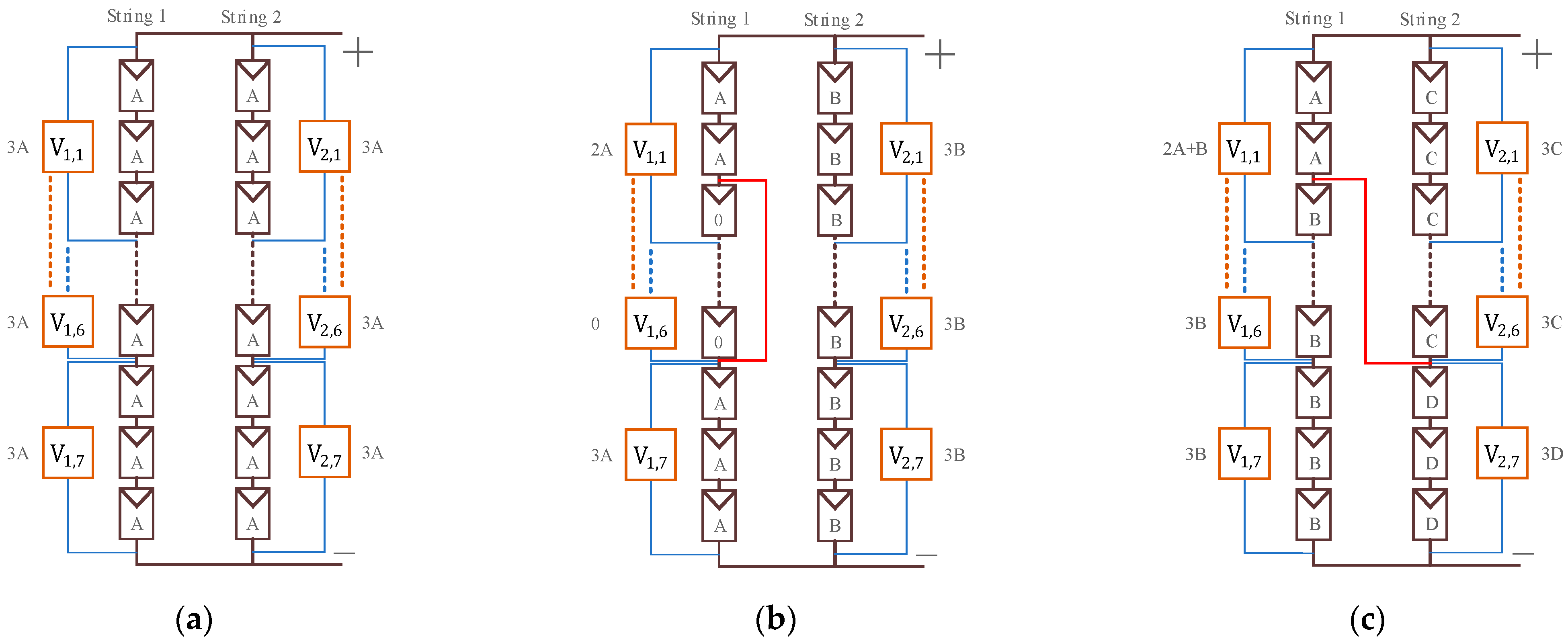
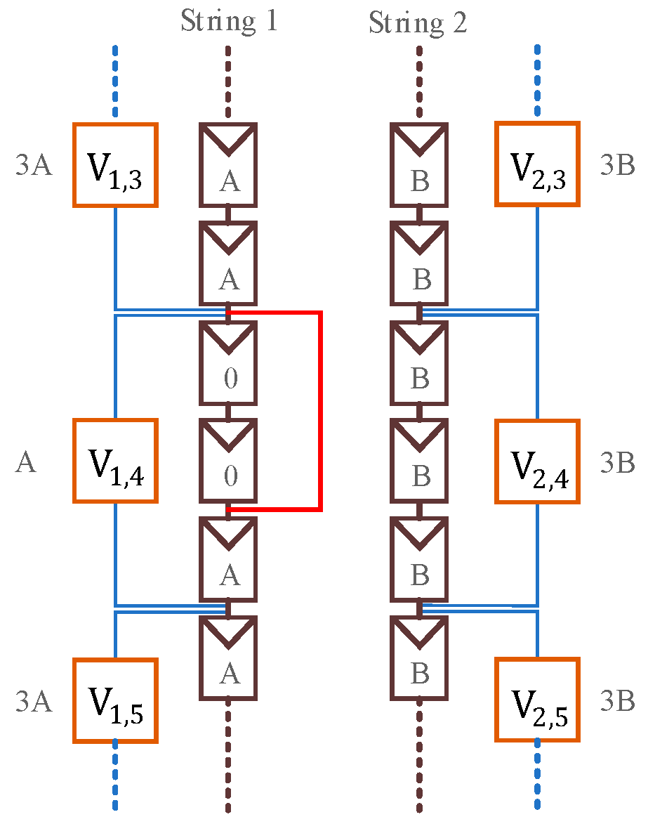
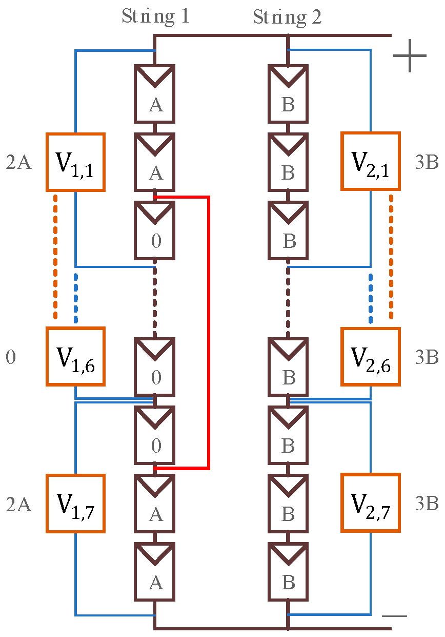
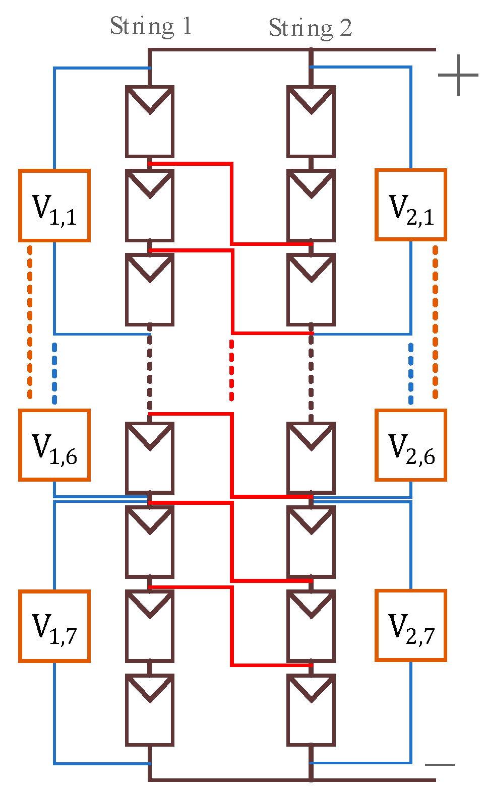
Assuming each module voltage is evenly distributed, each module group voltage will be identical during normal operation. This is shown in Figure 5a, with each group voltage at 3A. When a line-to-line short-circuit fault occurs, the voltages of each module group change differently. In Figure 5b, for an intra-string fault, the voltage of the affected module is 0 V. Therefore, in String 1, V_1,1 = 2A, V_1,2 − V_1,6 = 0, V_1,7 = 3A, while all module group voltages in String 2 remain at 3B. 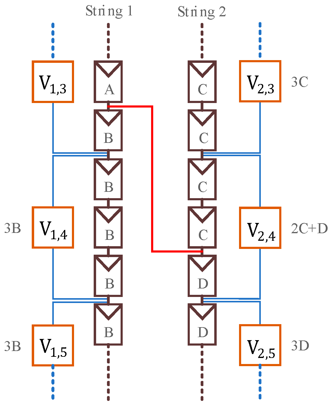In Figure 5c, for a cross-string fault, the array module voltages split into values A, B, C, and D, resulting in V_1,1 = 2A + B, V_1,2 − V_1,7 = 3B, V_2,1 − V_1,6 = 3C, and V_2,7 = 3D.

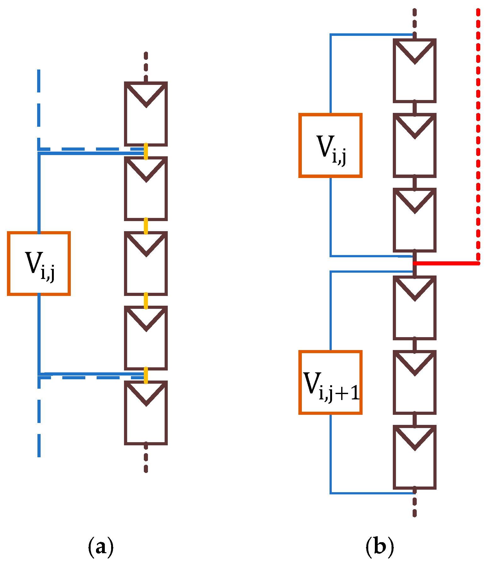
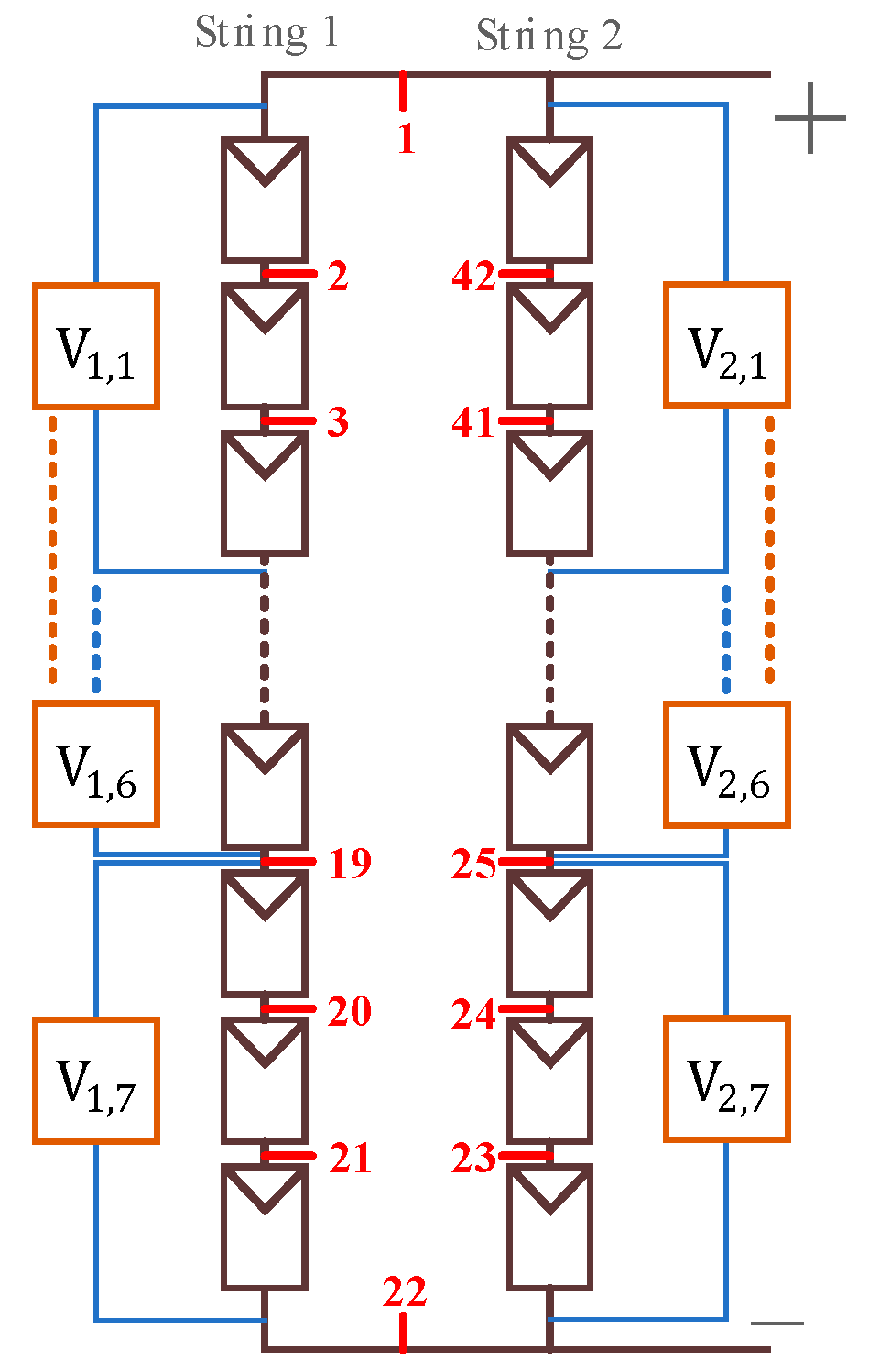
To identify all possible fault locations, a scanning method is used to compare the voltage of each module group with the voltage of the subsequent module group, calculating the rate of voltage change ∆V_i,j between them. This is shown in Equation (2).

$${∆V}_{i,j}={\displaystyle \frac{V_{i,j}-V_{i,j+1}}{V_{i,j}}}\times 100\%$$

(2)

When |∆V_i,j| exceeds the set threshold ∆V_threshold, this indicates that a line-to-line fault has occurred in one of the two module groups. Typically, the module voltage in the faulted group is lower than in normal modules, so the sign of ∆V_i,j must be determined. If ∆V_i,j is positive, this indicates that V_i,j+1 has a lower voltage, so the module with index j + 1 should be marked. Conversely, if ∆V_i,j is negative, this indicates that ∆V_i,j has a lower voltage, so the module with index j should be marked. This relationship is represented in Equation (3):

$$Marked index=\left\{\begin{array}{c} j+1 if {∆V}_{i,j}>0\\ j if {∆V}_{i,j}<0\end{array}\right.$$

(3)

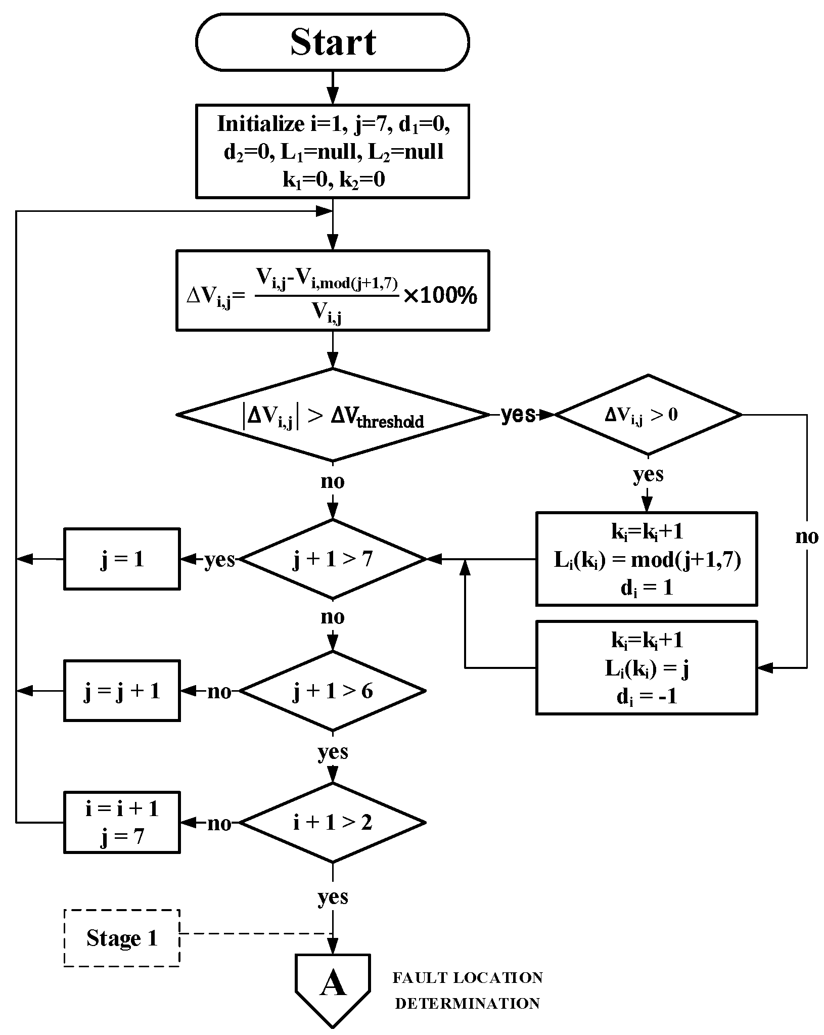
Using the 21 × 2 array configuration as an example, this study establishes a candidate location marking process for line-to-line short-circuit faults. This is shown in Figure 6. The scanning sequence starts from 7, followed by 7, 1, 2, …, 6. After calculating ∆V_i,j for the 6th module group, the process moves to the next row. The purpose of this sequence is to ensure that each module group undergoes calculation. To simplify the process, j + 1 is replaced with mod(j + 1).

In the candidate location marking process for line-to-line short-circuit faults shown in Figure 6, six additional variables are introduced: d₁, d₂, L₁, L₂, k₁, and k₂. Here, d₁ and d₂ represent the direction of module group voltages in the two strings. When a cross-string line-to-line short-circuit fault occurs, the module group voltages in the higher-potential string are ordered from high to low, whereas in the lower-potential string, the voltages are ordered from low to high. Thus, a direction value d of 1 for a string indicates that the fault point is the first recorded fault point in that string. Conversely, if d = −1, this indicates that the fault point is the last recorded fault point in that string, while a value of 0 indicates that no fault has occurred. Furthermore, L₁ and L₂ are sequences that record the fault candidate locations for each string. The remaining variables, k₁ and k₂, represent the number of fault candidate locations within each string.

3.2.2. Fault Location Determination

Through the previously described candidate location marking process for line-to-line short-circuit faults, this study obtains several pieces of information useful for determining the fault location: d₁, d₂, L₁, L₂, k₁, and k₂. Next, using the 21 × 2 array configuration as an example, this study presents the proposed fault location determination process for line-to-line short-circuit faults, as shown in Figure 7.

This process is derived from empirical observation and results in six cases, labeled Case 1 to Case 6. Cases 1 to 3 involve intra-string short-circuit faults, while Cases 4 to 6 involve cross-string short-circuit faults. Each of these six cases is explained in detail below.

Case 1: An intra-string short-circuit fault occurs within a single module group, as shown in Figure 8, with the fault occurring in module group V_1,4; two modules are short-circuited, resulting in a module group voltage of A. In the fault marking process, when i = 1, j = 3, a comparison between the third and fourth module groups reveals that |∆V_1,3| is greater than the threshold ∆V_threshold and is positive. Therefore, the fault position count k₁ is incremented by 1, the fault candidate array L₁ adds the index 4, and the voltage direction d₁ is set to 1. When j = 4, |∆V_1,4| also exceeds the threshold but is negative, so k₁ is incremented to 2, L₁ adds the index 4, and d₁ is set to −1. For i = 2, no anomalies are detected; therefore, the initial state is maintained. The results of the fault marking process are shown in

Table 2. Case 1 fault location process.

Stage 1
String #	ki	di	Li
i = 1	2	−1	4, 4
i = 2	0	0	null
Stage 2
String #	ki	di	Li
i = 1	1	−1	4
i = 2	0	0	null

, Stage 1.

Next, the process proceeds to the fault location determination step. Initially, duplicate fault points in the fault candidate array L_i are removed, and the remaining points are sorted. The fault point count k_i is then recalculated, with the results shown in Table 2, Stage 2. At this point, it has been determined that a fault point exists in the first string, so s is set at 1, with only one fault point present. Therefore, it is concluded that the fault is located in the fourth module group of the first string.

Case 2: An intra-string short-circuit fault occurs at the beginning and end module groups of the string, as shown in Figure 9. The fault is located between module groups V_1,1 and V_1,7. This type of fault is a more severe line-to-line short-circuit fault, as nearly the entire string is short-circuited, impacting the entire array’s power generation.

In the fault marking process, String 1 initially compares V_1,7 with V_1,1 and finds that both have the same voltage; therefore, no record is made. However, in the comparisons between V_1,1 and V_1,2, and between V_1,6 and V_1,7, it is observed that V_1,2 and V_1,6 have lower voltages, and these are recorded. Thus, a total of two module groups are marked as faulted, with the final recorded voltage direction as −1. No abnormalities are detected in String 2; therefore, it remains in its initial state. The marking results are shown in

Table 3. Case 2 fault location process.

Stage 1
String #	ki	di	Li
i = 1	2	−1	2, 6
i = 2	0	0	null
Stage 2
String #	ki	di	Li
i = 1	2	−1	2, 6
i = 2	0	0	null
Modified
String #	ki	di	Li
i = 1	2	−1	1, 7
i = 2	0	0	null

, Stage 1.

In the fault determination process, duplicate fault points in the fault candidate array L_i are first removed and sorted, and the fault point count k_i is recalculated, with the results shown in Table 3, Stage 2. At this stage, it has been found that there are two fault points in String 1, so s is set at 1. Directly identifying the fault in module groups 2 and 6 of String 1 would lead to an error. Therefore, whether the first marked point in L_s is less than or equal to 2 and the last marked point in L_s is greater than or equal to 6 will be checked first. If this condition is true, it is checked whether V_1,2 and V_1,6 are 0. If the condition is false, no further modifications are necessary. If the condition is true, this indicates that the fault is not in module groups 2 and 6, and the location results need to be adjusted by setting L_s(1) to 1 and L_s(k_s) to 7. This is shown in the “Modified” section of Table 3. Finally, it is determined that the fault location is in module groups 1 and 7 of String 1.

Case 3: Multiple module groups experience intra-string short-circuit faults, as shown in Figure 10. The fault occurs between module groups V_1,6 and V_1,7. In accordance with the fault marking process, in String 1, the initial comparison between V_1,7 and V_1,1 reveals that V_1,7 has a lower voltage; therefore, it is marked. The subsequently marked fault points are 6 and 7, resulting in a total of three fault points, with the final recorded voltage direction as 1. No abnormalities are detected in String 2. The results are shown in

Table 4. Case 3 fault location process.

Stage 1
String #	ki	di	Li
i = 1	3	1	7, 6, 7
i = 2	0	0	null
Stage 2
String #	ki	di	Li
i = 1	2	1	6, 7
i = 2	0	0	null

, Stage 1.

Next, in the fault determination process, duplicate fault points in the fault candidate array L_i are removed and sorted, and the fault point count k_i is recalculated. The results are shown in Table 4, Stage 2. At this stage, it is determined that there are two fault points in String 1, setting s to 1. However, the conditions L_s(1) <= 2 & L_s(k_s) >= 6 & V_s,2 = 0 & V_s,6 = 0 are not satisfied. Therefore, no modifications are needed, and the fault points are directly identified as being in module groups 6 and 7 of String 1.

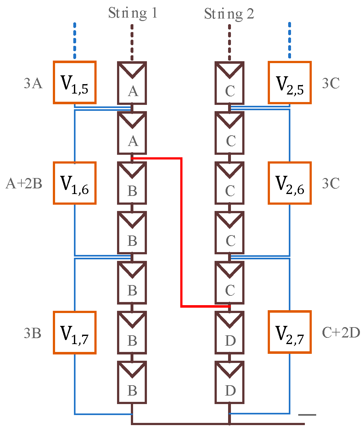
Case 4: A cross-string short-circuit fault occurs between two strings, with neither endpoint located in the first or last two module groups of each string, as shown in Figure 11. The fault occurs between module groups V_1,3 and V_2,4, so the voltages of all modules are divided into four values: A, B, C, and D.

In accordance with the fault marking process proposed in this paper, correctly marking the fault location requires knowledge of the relative magnitudes between A and B, as well as between C and D. This relationship can be determined through comparison. Using the fault structure in Figure 11 as an example, the array currents are labeled as shown in Figure 12.

In accordance with Kirchhoff’s Voltage Law, the sum of voltages in any closed loop is zero, resulting in the following equations:

$$\left\{\begin{array}{c} 8\times A=11\times C\\ 13\times B=10\times D\end{array}\right.$$

(4)

In accordance with the principle of proportionality, the following relationships are established:

$$\left\{\begin{array}{c} A>C\\ B<D\end{array}\right.$$

(5)

Based on the I–V characteristic curve of the PV module, it is understood that higher voltage corresponds to lower current, so:

$$\left\{\begin{array}{c} I_A<I_C\\ I_B>I_D\end{array}\right.$$

(6)

In accordance with Kirchhoff’s Current Law, the current flowing into any node is always equal to the current flowing out, implying that I_Fault must be greater than 0. Therefore:

$$\left\{\begin{array}{c} I_A<I_B\\ I_C>I_D\end{array}\right.$$

(7)

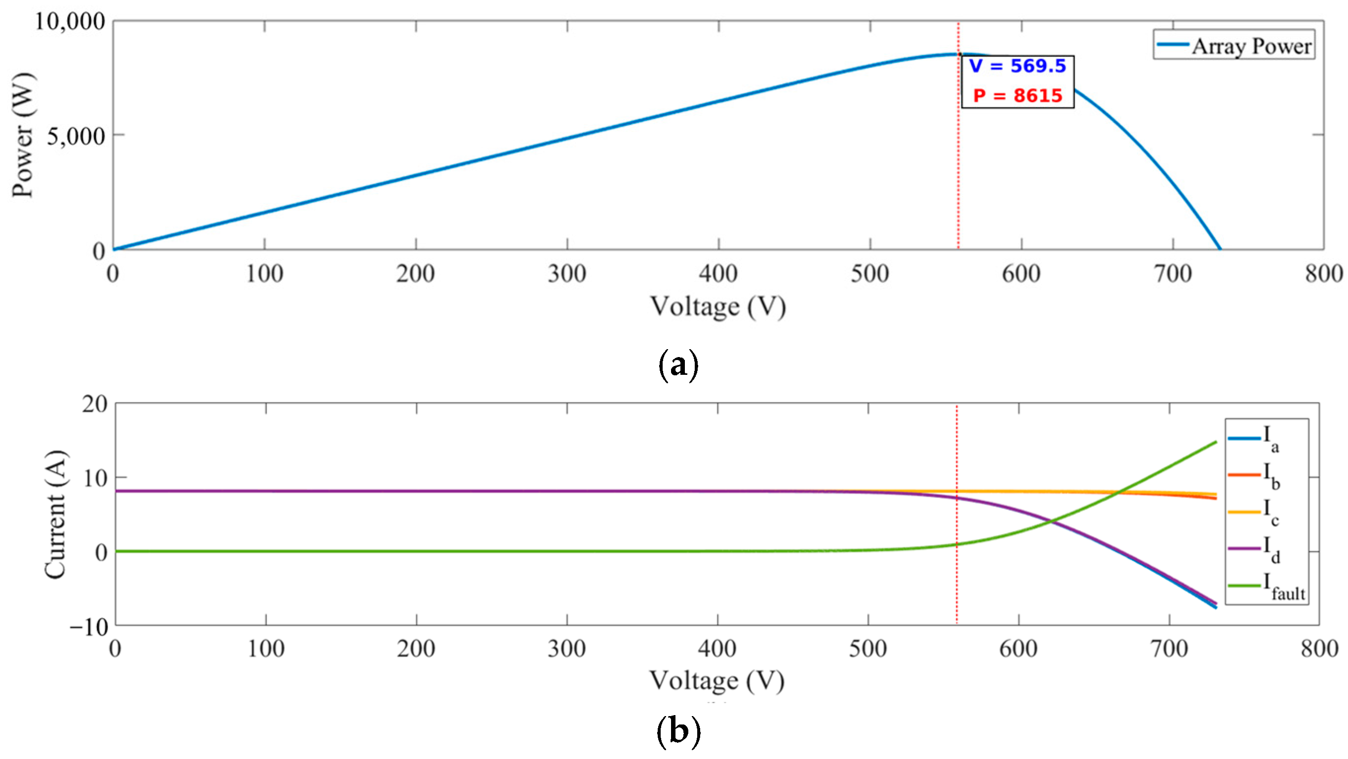
This inference is also confirmed by simulation, as shown in Figure 13. In Figure 13a, the simulation conditions are set to normal operating cell temperature (NOCT), with irradiance G at 800 W/m² and module temperature T at 45 °C. When the array reaches maximum power, the currents in Figure 13b exhibit the relationships described in Equations (6) and (7). Although I_Fault approaches 0 A at lower voltages, a closer inspection reveals that it remains greater than 0 A at all times.

Then, based on the I–V characteristic curve of the PV module, it can be concluded that:

$$\left\{\begin{array}{c} A>B\\ C<D\end{array}\right.$$

(8)

With the known voltage relationships between A and B, and C and D, the fault marking process is applied to the fault structure in Figure 11. In String 1, the fault points 7, 3, and 4 are sequentially marked, with the final recorded voltage direction as 1. In String 2, the fault points 1, 3, and 4 are marked in sequence, with the final recorded voltage direction as −1. The results are shown in

Table 5. Case 4 fault location process.

Stage 1
String #	ki	di	Li
i = 1	3	1	7, 3, 4
i = 2	3	−1	1, 3, 4
Stage 2
String #	ki	di	Li
i = 1	3	1	3, 4, 7
i = 2	3	−1	1, 3, 4

, Stage 1.

At the beginning of the fault determination process, the marked results are organized and sorted, as shown in Table 5, Stage 2. At this point, d₁ = 1 and d₂ = −1, so s is set to 1. Upon inspection, the last marked point in the low-potential string L₂ is not 6, and the first marked point in the high-potential string L₁ is not 2, indicating that the fault is located in the middle of both strings. Therefore, the fault location is identified as the first fault point in the high-potential string and the last fault point in the low-potential string. In this case, the fault is determined to be a short circuit between module group 3 in String 1 and module group 4 in String 2.

Case 5: A cross-string short-circuit fault occurs between two strings, with the low-potential end located in the last module group of the string, as shown in Figure 14. The fault occurs between module groups V_1,6 and V_2,7. The voltages of all modules are divided into four values, A, B, C, and D, with the same relative magnitudes as in Case 4.

Following the fault marking process, the results are shown in

Table 6. Case 5 fault location process.

Stage 1
String #	ki	di	Li
i = 1	3	1	7, 6, 7
i = 2	2	−1	1, 6
Stage 2
String #	ki	di	Li
i = 1	2	1	6, 7
i = 2	2	−1	1, 6
Modified
String #	ki	di	Li
i = 1	2	1	6, 7
i = 2	2	−1	1, 7

, Stage 1. In String 1, fault points 7, 6, and 7 are marked sequentially, with the final recorded voltage direction as 1. In String 2, fault points 1 and 6 are marked sequentially, with the final recorded voltage direction as −1.

The process then proceeds to fault marking, where duplicate fault points in the fault sequence L_i are removed and sorted, and the fault point count k_i is recalculated. The results are shown in Table 6, Stage 2, with d₁ = 1 and d₂ = −1, so s is set to 1. If the fault location is determined directly using the approach in Case 4, it will result in an error because the low-potential end fault point is located at the last fault point of that string. To accurately locate the fault, if the low-potential end is found in the second-to-last module group, it is necessary to first confirm whether the voltages of the second-to-last and third-to-last module groups are equal. In accordance with the premise of even voltage distribution, if the fault indeed occurs in the last module group, the voltages of the second-to-last and third-to-last module groups will be equal. Thus, when this condition is observed, the last fault point in the low-potential string should be adjusted to the last module group index to achieve an accurate fault location.

In Case 5, this condition is indeed confirmed, so the sequence L₂ is modified accordingly, as shown in Table 6, Modified. The fault location is then determined using the approach in Case 4, resulting in a short-circuit fault identified between module group 6 in String 1 and module group 7 in String 2.

Case 6: A cross-string short-circuit fault occurs between two strings, with the high-potential end located in the first module group of the string, as shown in Figure 15. The fault occurs between module groups V_1,1 and V_2,2. The voltages of all modules are divided into four values, A, B, C, and D, with the same relative magnitudes as in Case 4.

Following the fault marking process, the results are shown in

Table 7. Case 6 fault location process.

Stage 1
String #	ki	di	Li
i = 1	2	1	7, 2
i = 2	3	−1	1, 1, 2
Stage 2
String #	ki	di	Li
i = 1	2	1	2, 7
i = 2	2	−1	1, 2
Modified
String #	ki	di	Li
i = 1	2	1	1, 7
i = 2	2	−1	1, 2

, Stage 1. In String 1, fault points 7 and 2 are marked sequentially, with the final recorded voltage direction as 1. In String 2, fault points 1, 2, and 3 are marked sequentially, with the final recorded voltage direction as –1.

After entering the fault marking process, the marked results are organized as shown in Table 7, Stage 2; d₁ = 1 and d₂ = −1, so s is set to 1. When the high-potential end is located in the first module group of the string, the same issue as in Case 5 arises. However, in this case, the comparison is between the voltages of the second and third module groups in the high-potential string. If these two voltages are equal, this indicates that the fault is not in the first module group. Therefore, the first fault point in the high-potential string should be adjusted to the index of the first module group for accurate location. The modified results are shown in Table 7, Modified. The final fault location is determined to be a short circuit between module group 1 in String 1 and module group 2 in String 2.

In addition to the six PV array line-to-line short-circuit fault cases described above, Figure 7 (“Fault location determination process”) shows two situations in which fault location cannot be determined. The first case is when no fault location information is obtained during the fault marking process, making location impossible. This typically occurs when a short-circuit fault likely happens at both positive and negative endpoints of the array, causing all array voltages to read 0 V. The second case occurs when both d₁ and d₂ are either 1 or −1. This situation is unlikely under ideal conditions, as the relative magnitudes between the four voltage values (A, B, C, and D) in a cross-string fault are clearly defined, so this should not happen. Such a situation is more likely caused by multiple simultaneous faults; the heuristic fault location algorithm proposed in this paper cannot determine the fault location under these conditions.

3.2.3. Troubleshooting Scope

Having introduced the heuristic line-to-line fault location algorithm for six possible fault structures within a PV array, attention is turned to explaining the details to consider during line-to-line short-circuit troubleshooting. In the module group voltage measurement method proposed in this paper, the measurement scope is shown in Figure 16a. When a fault is located in module group V_i,j, it is necessary not only to inspect the three PV modules within that module group but also to examine the connecting segments between adjacent module groups, as indicated by the orange lines, to ensure that the fault is thoroughly addressed. Thus, when the fault occurs at the boundary between two module groups, as shown in Figure 16b, the fault location result may be V_i,j or V_i,j+1. Regardless of which of these is indicated as the fault location, troubleshooting must be conducted at the boundary to avoid overlooking any faults.

3.2.4. Threshold Determination

In the heuristic algorithm for line-to-line fault location, a critical component is appropriately setting the ∆V_threshold in the fault marking process. If ∆V_threshold is set too high, it may prevent milder faults from being accurately marked. Conversely, if ∆V_threshold is set too low, it could lead to unnecessary misjudgments. Therefore, determining the optimal ∆V_threshold is essential.

This section primarily explores how to set ∆V_threshold based on the array structure and the module group voltage measurement range. Typically, an intuitive approach is to set ∆V_threshold to be able to detect the mildest fault condition as a primary requirement. Therefore, using a 21 × 2 array configuration with three modules per module group as an example, this paper discusses the settings for both intra-string and cross-string line-to-line short-circuit faults.

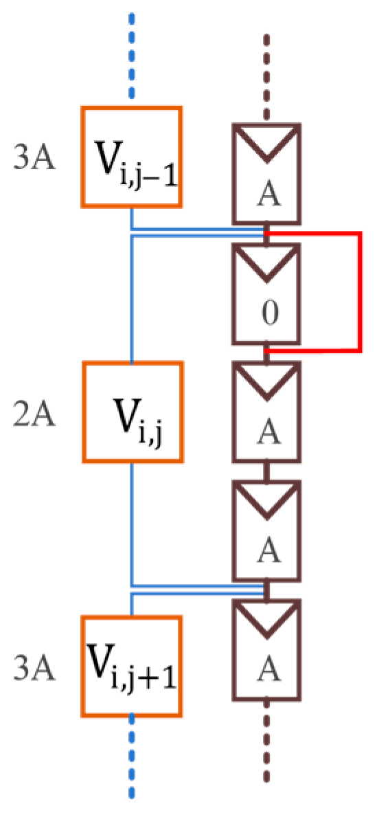
In the intra-string fault type, the mildest fault condition occurs when a single PV module experiences a short circuit, as shown in Figure 17. If a short-circuit fault occurs in module group V_i,j, the voltage change rates related to V_i,j are ∆V_i,j+1 and ∆V_i,j. Based on the voltage distribution, |∆V_i,j+1| can be calculated as 33.33%, and |∆V_i,j| as 50%. Therefore, in the intra-string fault type, the minimum ∆V_threshold should be set below 33.33%.

In the intra-string fault type, the mildest fault condition is also analyzed. As shown in Figure 18, a line-to-line short-circuit fault occurs between two strings with only one PV module difference. However, due to different positions, there are 19 possible fault scenarios from the top to the bottom of the array. The following section will simulate these 19 scenarios and calculate the minimum |∆V_i,j| for each case. In addition to the NOCT, the simulation environment parameters also explore four more extreme combinations of irradiance and module temperature: G = 100 W/m², T = 10 °C; G = 100 W/m², T = 85 °C; G = 1000 W/m², T = 10 °C; and G = 1000 W/m², T = 85 °C.

The simulation results are shown in

Table 8. Minimum |∆V_i,j| for cross-string short-circuit faults under different conditions.

Simulation Condition	Minimum |∆Vi,j| Among 19 Fault Locations
NOCT	2.4678%
G = 100 W/m2, T = 10 °C	2.1304%
G = 100 W/m2, T = 85 °C	2.7056%
G = 1000 W/m2, T = 10 °C	2.2019%
G = 1000 W/m2, T = 85 °C	2.8488%

, which indicate that |∆V_i,j| is lower at lower temperatures. The minimum |∆V_i,j| across all conditions occurs under the environment parameters G = 100 W/m², T = 10 °C, with a value of 2.1304%. Therefore, in the cross-string fault type, the minimum ∆V_threshold should be set below 2.1304% to ensure accurate fault location.

Finally, combining the minimum ∆V_threshold settings for both intra-string and cross-string fault types, this paper ultimately selects 2% as the ∆V_threshold for the 21 × 2 array configuration. This ensures that the heuristic line-to-line fault location algorithm can identify all possible fault locations.

The ∆V_threshold is primarily determined based on the array configuration and environmental conditions, as demonstrated for the 21 × 2 array in this study. For different array sizes or module groupings, the threshold should be recalibrated accordingly. Similarly, environmental factors such as irradiance and temperature affect the voltage differences and thus the threshold value. Developing adaptive thresholding techniques that automatically adjust to varying array configurations and operational conditions is an important direction for future research to improve the robustness and applicability of the proposed algorithm.

It is acknowledged that the proposed heuristic algorithm assumes relatively stable module voltage distributions under fault conditions. While minor environmental variations and measurement noise are mitigated through the use of module group voltage averages, significant fluctuations may affect accuracy. Robustness testing under various non-ideal conditions and incorporation of filtering or adaptive thresholding techniques are important future research directions to enhance practical applicability.

4. Simulation Test and Discussion

Furthermore, this paper uses MATLAB/Simulink to conduct simulation tests to verify the accuracy of the heuristic line-to-line fault location algorithm in locating faults within the PV array, then discusses the test results. First, each line segment in the 21 × 2 PV module array is numbered counterclockwise, as shown in Figure 19, with the entire array sequentially numbered from 1 to 42. Second, a fault test point reference table based on the troubleshooting scope of each module group is created, as shown in

Table 9. Reference table for module groups and fault test point numbers.

Module Group #	Fault Test Point #	Module Group #	Fault Test Point #
V1,1	1, 2, 3, 4	V2,1	1, 40, 41, 42
V1,2	4, 5, 6, 7	V2,2	37, 38, 39, 40
V1,3	7, 8, 9, 10	V2,3	34, 35, 36, 37
V1,4	10, 11, 12, 13	V2,4	31, 32, 33, 34
V1,5	13, 14, 15, 16	V2,5	28, 29, 30, 31
V1,6	16, 17, 18, 19	V2,6	25, 26, 27, 28
V1,7	19, 20, 21, 22	V2,7	22, 23, 24, 25

. Finally, short-circuit fault location tests are conducted between points using the NOCT environment parameters.

The simulation test results for line-to-line fault location are shown in Figure 20. Here, P1 and P2 represent the two endpoints of a line-to-line fault, varying from 1 to 42. Green cells with a recorded value of 1 indicate successful fault location, while red cells with a recorded value of −1 indicate failures to locate faults. The figure shows that most fault scenarios are successfully located by the heuristic line-to-line fault location algorithm, though it still cannot locate some faults. The diagonal from the top-left to the bottom-right represents scenarios where P1 and P2 are at the same test point, indicating no actual fault and thus no location being found, which is regarded as normal. The diagonal from the top-right to the bottom-left represents cases where the endpoints of the line-to-line fault are in different strings but share the same potential, so no fault characteristics are reflected in the module group voltages, resulting in no location being found. In addition, there are two unlocatable cases in the middle left and top middle of the figure, where P1 = 1, P2 = 22 and P1 = 22, P2 = 1, respectively. These represent faults caused by a short circuit between the positive and negative terminals of the array’s total output. This will cause all module voltages to read 0 V, preventing the fault location algorithm from accurately locating the fault.

Finally, the overall fault location success rate is calculated as shown in Equation (9). The denominator is the total of 42 × 42 = 1764 combinations, minus 42 non-fault scenarios, resulting in a base of 1722. The numerator is the number of combinations successfully located. Subtracting an additional 40 combinations with the same potential and 2 instances of short-circuit between the array’s positive and negative terminals, the effective denominator is 1680. The calculated success rate is 97.56%.

$$Success Rate={\displaystyle \frac{42\times 42-42-40-2}{42\times 42-42}}\times 100\%=97.56\%$$

(9)

Compared with existing literature, the proposed heuristic algorithm demonstrates significant improvements in fault localization precision and practical applicability. While many prior studies, such as Hasan et al. [16] and Suliman et al. [17], have achieved high fault detection accuracy using machine learning classifiers, their methods often require large training datasets and complex computational resources, limiting real-time applicability. The approach by Jia et al. [15] effectively isolates affected strings but does not achieve localization at the module group level, which is critical for reducing maintenance scope. In contrast, fault location is narrowed down to a specific module group by the proposed method, substantially reducing the inspection and repair time.

In addition to the reported fault location success rate of 97.56%, the simulation results identify specific failure modes such as faults at both array terminals causing all zero voltages and faults involving same-potential endpoints, which are inherently undetectable by the proposed method. While false positive and false negative rates are not explicitly calculated in this study, the low complexity and heuristic nature of the algorithm contribute to fast computational performance, suitable for real-time applications. Detailed analysis of error rates and algorithmic robustness under varying operational conditions will be pursued in future work.

5. Conclusions

This paper successfully developed and validated a heuristic algorithm for line-to-line fault location based on module group voltage measurement, aimed at addressing the problem of locating line-to-line short-circuit faults in PV arrays, achieving the following key outcomes:

• By utilizing the characteristic that line-to-line short-circuit faults do not create multiple maximum power points in the P-V curve, this study investigates the phenomenon of line-to-line short-circuit faults at maximum power generation in the array by extracting the P-V curve.
• Using a 21 × 2 PV module array configuration, this study examines six cases of two types of line-to-line short-circuit faults: intra-string and cross-string. Based on empirical rules, a heuristic algorithm for line-to-line fault location based on module group voltage measurement is proposed.
• Simulation tests conducted through MATLAB/Simulink reveal that the heuristic line-to-line fault location algorithm can successfully locate most line-to-line short-circuit faults, reducing the troubleshooting scope to within a single module group, with a success rate of approximately 97.56%.
• The line-to-line fault location method proposed in this paper is intuitive, simple, and fast. Although the location process is illustrated using a 21 × 2 PV array, it can be adapted for different applications and various array sizes. Moreover, the module group size for voltage measurement can be adjusted based on the required location accuracy.
• The importance of this work lies in its practical applicability and economic benefits. By enabling precise fault localization using only module group voltage measurements, maintenance teams can reduce inspection time by approximately 80% compared to manual whole-array inspection. This translates to significant cost savings for large-scale PV installations, where arrays may contain thousands of modules spread over vast areas. Furthermore, the algorithm’s simplicity and low computational requirements make it suitable for integration into existing PV monitoring systems without substantial hardware upgrades. As the global PV capacity continues to grow, such efficient fault localization methods become increasingly critical for maintaining system reliability and safety.
• Despite the high success rate, the proposed algorithm has certain limitations:
  • It cannot locate faults when both array terminals are short-circuited, causing all voltages to read 0 V.
  • It assumes relatively uniform voltage distribution among modules, which may not hold under severe partial shading.
  • It is designed for single line-to-line faults and may not accurately locate multiple simultaneous faults.
  • The threshold determination requires prior knowledge of array configuration and environmental conditions.
  • Future research should focus on extending the algorithm to handle multiple fault scenarios, integrating machine learning for adaptive threshold determination, and field validation in large-scale PV installations. The proposed method represents a significant step toward automated, efficient PV system maintenance, with potential applications in utility-scale solar farms where rapid fault location is critical for minimizing revenue losses.

References

1. IRENA. Renewable Energy Statistics 2021; The International Renewable Energy Agency: Abu Dhabi, United Arab Emirates, 2021. [Google Scholar]
2. Zhao, Y.; de Palma, J.; Mosesian, J.; Lyons, R.; Lehman, B. Line–Line Fault Analysis and Protection Challenges in Solar Photovoltaic Arrays. IEEE Trans. Ind. Electron. 2013, 60, 3784–3795. [Google Scholar] [CrossRef]
3. Alam, M.K.; Khan, F.; Johnson, J.; Flicker, J. A Comprehensive Review of Catastrophic Faults in PV Arrays: Types, Detection, and Mitigation Techniques. IEEE J. Photovolt. 2015, 5, 982–997. [Google Scholar] [CrossRef]
4. Alam, M.K.; Khan, F.H.; Johnson, J.; Flicker, J. PV faults: Overview, modeling, prevention and detection techniques. In Proceedings of the 2013 IEEE 14th Workshop on Control and Modeling for Power Electronics (COMPEL), Salt Lake City, UT, USA, 23–26 June 2013; pp. 1–7. [Google Scholar] [CrossRef]
5. Walker, H.A. Best Practices for Operation and Maintenance of Photovoltaic and Energy Storage Systems, 3rd ed.; National Renewable Energy Lab (NREL): Golden, CO, USA, 2018. [Google Scholar] [CrossRef]
6. Gunda, T.; Hackett, S.; Kraus, L.; Downs, C.; Jones, R.; McNalley, C.; Bolen, M.; Walker, A. A Machine Learning Evaluation of Maintenance Records for Common Failure Modes in PV Inverters. IEEE Access 2020, 8, 211610–211620. [Google Scholar] [CrossRef]
7. Pillai, D.S.; Blaabjerg, F.; Rajasekar, N. A Comparative Evaluation of Advanced Fault Detection Approaches for PV Systems. IEEE J. Photovolt. 2019, 9, 513–527. [Google Scholar] [CrossRef]
8. Wang, Z.; McConnell, S.; Balog, R.S.; Johnson, J. Arc fault signal detection—Fourier transformation vs. wavelet decomposition techniques using synthesized data. In Proceedings of the 2014 IEEE 40th Photovoltaic Specialist Conference (PVSC), Denver, CO, USA, 8–13 June 2014; pp. 3239–3244. [Google Scholar]
9. Kim, K.A.; Seo, G.-S.; Cho, B.-H.; Krein, P.T. Photovoltaic hot-spot detection for solar panel substrings using AC parameter characterization. IEEE Trans. Power Electron. 2016, 31, 1121–1130. [Google Scholar] [CrossRef]
10. Rezgui, W.; Mouss, N.K.; Mouss, L.; Mouss, M.D.; Amirat, Y.; Benbouzid, M. Smart diagnosis algorithm of the open-circuit fault in a photovoltaic generator. In Proceedings of the 2015 3rd International Conference on Control, Engineering & Information Technology (CEIT), Tlemcen, Algeria, 25–27 May 2015; pp. 1–5. [Google Scholar]
11. Quater, P.B.; Grimaccia, F.; Leva, S.; Mussetta, M.; Aghaei, M. Light Unmanned Aerial Vehicles (UAVs) for Cooperative Inspection of PV Plants. IEEE J. Photovolt. 2014, 4, 1107–1113. [Google Scholar] [CrossRef]
12. Roy, S.; Alam, M.K.; Khan, F.; Johnson, J.; Flicker, J. An Irradiance-Independent, Robust Ground-Fault Detection Scheme for PV Arrays Based on Spread Spectrum Time-Domain Reflectometry (SSTDR). IEEE Trans. Power Electron. 2018, 33, 7046–7057. [Google Scholar] [CrossRef]
13. Takashima, T.; Yamaguchi, J.; Otani, K.; Oozeki, T.; Kato, K.; Ishida, M. Experimental studies of fault location in PV module strings. Sol. Energy Mater. Sol. Cells 2009, 93, 1079–1082. [Google Scholar] [CrossRef]
14. Hong, Y.-Y.; Pula, R.A. Methods of Photovoltaic Fault Detection and Classification: A Review. Energy Rep. 2022, 8, 5898–5929. [Google Scholar] [CrossRef]
15. Jia, K.; Shi, Z.; Wu, W.; Chen, J.; Bi, J.; Bi, T. Incipient Fault Identification-Based Protection for a Photovoltaic DC Integration System. IEEE Trans. Power Deliv. 2022, 37, 1660–1670. [Google Scholar] [CrossRef]
16. Hasan, H.A.; Shehab, M.A.; Al-Gizi, A. Detecting and Classifying Line-to-Line Fault in Photovoltaic Arrays Under Challenging Conditions Using Machine Learning Classifiers. Int. J. Intell. Eng. Syst. 2024, 17, 263–273. [Google Scholar]
17. Suliman, F.; Anayi, F.P.; Packianather, M. Electrical Faults Analysis and Detection in Photovoltaic Arrays Based on Machine Learning Classifiers. Sustainability 2024, 16, 1102. [Google Scholar] [CrossRef]
18. Arunachalam, V.; Karthickraja, J.; Senthamizh Selvan, S. Wavelet transform based detection, classification and location of faults in a PV array. J. Ambient. Intell. Hum. Comput. 2023, 14, 11227–11237. [Google Scholar] [CrossRef]
19. Miao, W.; Luo, Y.; Wang, F.; Jiang, C. Fault Detection and Location Algorithm by Voltage Characteristics for PV System. IEEE J. Photovolt. 2023, 13, 968–978. [Google Scholar] [CrossRef]
20. Sepúlveda-Oviedo, E.H.; Travé-Massuyès, L.; Subias, A.; Pavlov, M.; Alonso, C. Fault Diagnosis of Photovoltaic Systems Using Artificial Intelligence: A Bibliometric Approach. Heliyon 2023, 9, e21491. [Google Scholar] [CrossRef]
21. Yang, C.; Sun, F.; Zou, Y.; Lv, Z.; Xue, L.; Jiang, C.; Liu, S.; Zhao, B.; Cui, H. A Survey of Photovoltaic Panel Overlay and Fault Detection Methods. Energies 2024, 17, 837. [Google Scholar] [CrossRef]
22. Yi, Z.; Etemadi, A.H. Line-to-Line Fault Detection for Photovoltaic Arrays Based on Multiresolution Signal Decomposition and Two-Stage Support Vector Machine. IEEE Trans. Ind. Electron. 2017, 64, 8546–8556. [Google Scholar] [CrossRef]
23. Niu, S.; Zhao, Q.; Niu, S.; Jian, L. A Comprehensive Investigation of Thermal Risks in Wireless EV Chargers Considering Spatial Misalignment from a Dynamic Perspective. IEEE J. Emerg. Sel. Top. Ind. Electron. 2024, 5, 1560–1571. [Google Scholar] [CrossRef]
24. Farivar, G.; Asaei, B. Photovoltaic module single diode model parameters extraction based on manufacturer datasheet parameters. In Proceedings of the 2010 IEEE International Conference on Power and Energy, Kuala Lumpur, Malaysia, 29 November–1 December 2010; pp. 929–934. [Google Scholar]
25. Hejri, M.; Mokhtari, H.; Azizian, M.R.; Ghandhari, M.; Söder, L. On the Parameter Extraction of a Five-Parameter Double-Diode Model of Photovoltaic Cells and Modules. IEEE J. Photovolt. 2014, 4, 915–923. [Google Scholar] [CrossRef]
26. Kreft, W.; Przenzak, E.; Filipowicz, M. Photovoltaic chain operation analysis in condition of partial shading for systems with and without bypass diodes. Int. J. Light Electron Opt. 2021, 247, 167840. [Google Scholar] [CrossRef]
27. Pei, T.; Hao, X. A Fault Detection Method for Photovoltaic Systems Based on Voltage and Current Observation and Evaluation. Energies 2019, 12, 1712. [Google Scholar] [CrossRef]
Figure 1. Equivalent circuit of single-diode model.
Applsci 15 06366 g001
Figure 2. Array size of the PV module used.
Applsci 15 06366 g002
Figure 3. Schematic diagram showing line-to-line fault.
Applsci 15 06366 g003
Figure 4. P–V characteristic curves of PV array under different conditions.
Applsci 15 06366 g004
Figure 5. Module group voltage under different conditions. (a) normal operation; (b) intra-string fault; (c) cross-string fault.
Applsci 15 06366 g005
Figure 6. Candidate location marking process for line-to-line short-circuit faults.
Applsci 15 06366 g006
Figure 7. Fault location determination process for line-to-line short-circuit faults.
Applsci 15 06366 g007
Figure 8. Case 1 fault.
Applsci 15 06366 g008
Figure 9. Case 2 fault.
Applsci 15 06366 g009
Figure 10. Case 3 fault.
Applsci 15 06366 g010
Figure 11. Case 4 fault.
Applsci 15 06366 g011
Figure 12. Cross-string fault current.
Applsci 15 06366 g012
Figure 13. Experimental results under NOCT conditions. (a) Array P–V curve; (b) current curves.
Applsci 15 06366 g013
Figure 14. Case 5 fault.
Applsci 15 06366 g014
Figure 15. Case 6 fault.
Applsci 15 06366 g015
Figure 16. Fault location troubleshooting scope (a) module group voltage measurement range; (b) fault endpoint located between two module groups.
Applsci 15 06366 g016
Figure 17. Illustration of the mildest intra-string short-circuit fault.
Applsci 15 06366 g017
Figure 18. Illustration of the mildest cross-string short-circuit fault.
Applsci 15 06366 g018
Figure 19. Schematic diagram showing the numbering for the test array.
Applsci 15 06366 g019
Figure 20. Simulation test results for line-to-line fault location.
Applsci 15 06366 g020