Article

A GNSS–Cellular Network Hybridization Strategy for Robust Positioning

by
María Jesús Jiménez-Martínez
1,*,
Mónica Zabala Haro
1,2,
Ángel Martín Furonés
1 and
Ana Anquela Julián
1
1
Department of Cartographic, Geodesy and Photogrammetry Engineering, Higher Technical School of Geodetic, Cartographic and Topographical Engineering, Universitat Politècnica de València, Campus de Vera s/n, 46022 Valencia, Spain
2
Telecommunications Engineering School, Faculty of Computer Science and Electronics, Escuela Superior Politécnica de Chimborazo (ESPOCH), Campus Chimborazo, Riobamba EC060155, Ecuador
*
Author to whom correspondence should be addressed.
Appl. Sci. 2025, 15(11), 6300; https://doi.org/10.3390/app15116300
Submission received: 14 April 2025 / Revised: 26 May 2025 / Accepted: 28 May 2025 / Published: 4 June 2025
(This article belongs to the Special Issue Mapping and Localization for Intelligent Vehicles in Urban Canyons)

Abstract

:

Featured Application

As mobile communication technology advances, particularly with the deployment of 4G and 5G networks, the positioning capabilities provided by cellular networks are becoming increasingly accurate. This work presents a hybrid localization approach that allows user equipment (UE) to autonomously combine Global nNavigation satellite system (GNSS) and 4G/5G data to improve positioning, especially in urban canyons and indoor environments where GNSS signals are weak or unavailable. The developed method enhances user-level decision making based on positioning precision and reliability. As mobile devices evolve and cellular network accuracy improves, this hybridization approach is expected to play a critical role in future applications such as smart mobility, emergency responses, augmented reality, and autonomous systems, where robust and continuous positioning is essential.

Abstract

The hybridization of cellular networks and GNSS systems has gained increasing attention, especially in urban canyons and indoor environments where GNSS performance degrades significantly. Hybrid localization is part of the 3rd Generation Partnership Project (3GPP) standard, offering an effective solution when satellite visibility is limited. Additional cellular measurements can enhance the accuracy and reliability of standalone UE. Hybrid methods offer multiple benefits: an improved availability, continuity, and integrity; better signal penetration due to proximity; a lower power consumption; and, in harsh environments, potentially more accurate positioning than a GNSS. Moreover, GNSS chipsets in mobile phones or smartwatches are typically power-intensive. This work presents a user-level hybridization method that enables UE to receive both GNSS and 4G/5G data and autonomously determine whether to apply hybrid positioning. The developed algorithms improve the precision and reliability, allowing user-driven decisions based on data quality. The system was tested under static conditions across various scenarios: outdoors, in urban canyons, and indoors. The results show that, while hybridization enhances positioning, the 4G-only solution often performs in terms of vertical accuracy. Standard deviation metrics help guide the selection of the most precise option in real time.

1. Introduction

By the end of 2024, approximately 4.88 billion people owned smartphones, representing 60.42% of the global population [1]. According to the latest GSA GNSS Market Report [2], the number of smartphones equipped with GNSS capabilities is projected to increase from 6.4 billion in 2019 to 9.6 billion by 2029. Currently, 4G technology accounts for 60% of global mobile connections, and 5G is projected to reach 1.2 billion smartphone connections by 2025 [3].
In the United States, the Federal Communications Commission (FCC) [4] plays a central role in telecommunications regulation and participates in the standardization efforts led by the 3GPP [5]. Through legislation such as the Wireless Communications and Public Safety Act of 1999 (911 Act) [6], the FCC mandated mobile emergency call infrastructure. Phase I required reporting the caller’s phone number and cell tower location, while Phase II introduced more precise location data (latitude, longitude, and altitude) within 50–300 m when a GNSS is available. The updates in 2012 under the Next Generation 911 initiative further addressed indoor positioning [7].
3GPP develops globally standardized specifications across multiple generations of mobile networks, including GSM (2G), UMTS (3G), LTE (4G), and NR (5G) [8]. The 5G positioning architecture builds upon LTE while maintaining backward compatibility [9]. Technical specification TS 36.305 V17.3.0 defines location services (LCSs) for LTE, detailing architecture, protocols, and methods like E-CID, A-GNSS, DL-TDOA, UL-TDOA, and RTT, which rely on signal-based measurements (ToA, TDoA, AoA, RSS, etc.) [10,11,12]. These are further enhanced using technologies such as Wi-Fi, Bluetooth, barometric sensors, and inertial motion data.
Hybrid positioning, defined in the LTE standard [10], integrates multiple methods to enhance the accuracy and reliability, particularly in challenging environments like urban canyons or indoor areas with limited satellite visibility. Hybrid methods enhance the availability, continuity, and integrity, while reducing power consumption in mobile GNSS chipsets [13,14,15]. They are especially valuable where 4G/5G outperforms a GNSS, such as in non-line-of-sight (NLoS) or multipath-prone environments.
While 3GPP provides a framework for hybrid positioning, it does not prescribe specific algorithms [13,16,17]. These are typically developed independently by mobile network providers. Moreover, since most positioning measurements are not accessible on commercial devices, research into hybridization often relies on simulations or emulated environments [16,18,19,20]. Recent studies [11,21,22,23] have highlighted the effectiveness of hybrid and trilateration-based approaches. In addition, more recent contributions have explored alternative fusion models and control-oriented strategies to enhance the robustness in the presence of non-Gaussian noise and outliers. For instance, Feng et al. [24] presented an adaptive fusion method combining IMU and UWB data, explicitly addressing non-line-of-sight scenarios using dynamic weight adjustments and outlier suppression techniques. Similarly, Garraffa et al. [25] proposed a localization framework based on parallel robot kinematics as an alternative to traditional trilateration, introducing geometric constraints that improved the stability under degraded conditions. These approaches offer complementary perspectives to the present user-level GNSS–cellular hybridization strategy and reinforce the importance of resilient fusion schemes in modern positioning systems.
This study proposes two novel hybridization methods at the user level: position-level hybridization and measurement-level hybridization. While hybrid positioning techniques are already employed by mobile network operators within their infrastructure, the novelty of this work lies in implementing such methods directly on the user’s device, without relying on network-side processing. This user-centric approach enables standalone positioning improvements using only data collected by the smartphone, making the solution accessible, transparent, and independent of proprietary implementations by service providers.
The position-level hybridization method combines UE coordinates (latitude, longitude, ellipsoidal height, and associated precision) obtained from 4G/5G mobile networks with GNSS data. Both data sources were collected using the CellTracker Android 10 app [26], which is based on Google’s official geolocation API. The measurement-level hybridization method fuses GNSS pseudoranges with 4G/5G cellular-derived ranging measurements into a unified system of positioning equations. GNSS pseudoranges were obtained using the Geo RINEX Logger app, which stores Receiver Independent Exchange (RINEX) files recorded by the smartphone’s GNSS receiver [27]. The 4G/5G cellular ranging measurements, however, had to be indirectly derived from the coordinates provided by mobile networks, since raw cellular pseudorange data are not accessible to end users and are only available to mobile network operators.
These algorithms were evaluated in terms of their accuracy and precision through static tests conducted in outdoor, urban canyon, and indoor scenarios, using a known reference position as a benchmark. The proposed methods represent user-level hybridization strategies that enhance the robustness of the positioning performance under diverse environmental conditions.
The rest of this paper is organized as follows: Section 2 presents the data sources and methods used. Section 3 analyzes the performance through numerical experiments. Section 4 discusses the findings and concludes the study.

2. Materials and Methods

Hybrid positioning is a technique used to determine a device’s or user’s geographic location by combining multiple positioning methods and technologies, leveraging the strengths of each to improve the overall accuracy and reliability. This is accomplished through sophisticated algorithms that assess the accuracy and availability of each positioning source in real time to provide the most reliable and precise location estimate. Since the measurements are affected by noise (e.g., receiver noise, multipath) and the applied models are not perfect, adjustment techniques are required for accurate position parameter estimation.
The proposed hybridization methods are based on trilateration and include adjustments using the deterministic Gaussian method with coordinate increments, as described in [28,29]. These methods integrate GNSS data and 4G/5G mobile network measurements into a mathematical model represented by a system of observation equations [30], which is then used to estimate the position of the UE.
The two proposed hybridization strategies are designed to operate at different levels of abstraction, which has important implications for both their implementation and their capacity to model measurement errors. The position-level hybridization method combines geodetic coordinates (x, y, z), independently provided by the GNSS chipset and the cellular network. These coordinates are internally processed and corrected by the respective systems, and thus do not allow for the direct modeling of physical-layer error sources such as multipath, ionospheric delays, or signal strength variations. In contrast, the measurement-level hybridization method works with GNSS pseudoranges and cellular distances computed between the user equipment (UE) and the base stations (BSs). However, it is important to note that, in this case, the BS–UE pseudoranges are not directly measured, but simulated or inferred based on network-side position estimates, and therefore, they may not fully reflect raw radio signal characteristics. These differences impose distinct constraints on the error-modeling capabilities of each method and motivate the structure of the two independent estimation frameworks described in the following subsections.

2.1. Position-Level Hybridization Method

This method combines position estimates from the mobile network—denoted as ( x 4 G / 5 G , y 4 G / 5 G , z 4 G / 5 G ) —and from the GNSS sensor of the smartphone—denoted as ( x G N S S , y G N S S , z G N S S ) . These two sources of data are independent and the fusion is performed in the coordinate domain.
The latitude, longitude, and altitude values from the 4G/5G mobile network are obtained using the CellTracker app. These coordinates are originally provided in a geocentric reference frame and are then transformed to the UTM projection. For this study, they were further expressed in the local east–north–up (ENU) coordinate system, and are referred to as x, y, and z throughout this manuscript.
The mathematical model of this method, which is well established in the literature [30,31], can be expressed in matrix form as follows:
A · x = b + υ
where the coefficient matrix A is
A = 1 0 0 0 1 0 0 0 1 1 0 0 0 1 0 0 0 1 . . . 1 0 0 0 1 0 0 0 1 3 n x 3
The vector of unknown variables (corrections) is
x = d x d y d z 3 x 1
The vector of independent terms b , with n observations for the x, y, and z coordinates, is
b n x , y , z = b 1 x b 1 y b 1 z . · . b n x b n y b n z 3 n x 1
  • b n x = x o b s ,   n x i n i t ;
  • b n y = y o b s ,   n y i n i t ;
  • b n z = z o b s ,   n z i n i t .
The initial values of x i n i t , y i n i t , and z i n i t are calculated as the average of the n observed data. The vector υ represents the residuals.
The weighted least-squares (WLS) method allows specific weights to be assigned to each equation. The mathematical model (1) can then be written as follows:
P · ( A · x ) = P · ( b + υ )
where P   is the diagonal weight matrix of the n observations:
P = 1 σ 1 x 2 0 0 0 0 0 0 0 0 0 1 σ 1 y 2 0 0 0 0 0 0 0 0 0 1 σ 1 z 2 0 0 0 0 0 0 · · · · · · · · · · · · · · · · · · · · · · · · · · · 0 0 0 0 0 0 1 σ n x 2 0 0 0 0 0 0 0 0 0 1 σ n y 2 0 0 0 0 0 0 0 0 0 1 σ n z 2 3 n x 3 n
Each diagonal element of P is a function of the precision value provided by the Cell Tracker app:
σ ^ n 2 = σ 0 2 ( a c c u r a c y   o f   n   o b s e r v a t i o n ) 2
where σ 0 2 is a constant variance value.
In Equation (7), the accuracy of each observation is obtained from the CellTracker app, which reports a set of estimated coordinates (x, y, z) together with an associated accuracy value. This value reflects the uncertainty of the position estimate for each set of GNSS or 4G data, depending on the source used. The scalar factor σ02 represents a global variance term, computed as the average of all the reported accuracy values observed throughout the experimental campaign. This global factor serves as a representative characterization of the overall noise level in the system and is used to scale the observation weights.
The WLS solution for the unknown vector x is as follows:
x = ( A T · P · A ) 1 · A T · P · b
The residual vector υ vector is then given by the following:
υ = A · x b  
To remove outliers or blunders from the observations, a threshold is applied to the residuals:
υ > p · υ a l l
where,
  • υ is the residual from Equation (9);
  • υ a l l is the mean of all residuals;
  • p is a user-defined threshold parameter, e.g., p = 2.5 .
The variance–covariance matrix Σ x represents the accuracy of the WLS solution:
Σ x =   σ 0 2 · ( A T · P · A ) 1
where the a posteriori variance factor σ 0 P 2   is computed as follows:
σ 0 P 2 = υ T · P · υ n m
Here, n is the number of observations and m is the number of unknowns.
The diagonal elements of Σ x   are σ x x 2 , σ y y 2 ,   a n d   σ z z 2 and they represent the variances in the local ENU coordinate system.
Finally, the standard deviations are calculated as follows:
σ x = σ x x 2 ,   σ y = σ y y 2 ,       σ z = σ z z 2
These values are used to assess and compare the positioning performance of the GNSS-4G/5G hybridization solution, the standalone GNSS solution, and the standalone 4G/5G solution.
It is important to note that, in Equation (4), each observation value in the vector of independent terms b corresponds to a single epoch, and only one (x, y, z) coordinate is available per epoch for each source (GNSS or 4G/5G). As a result, a single epoch does not provide enough information to resolve the hybrid positioning system independently. Therefore, measurements from multiple consecutive epochs are accumulated and processed together to ensure system solvability and enhance the robustness.

2.2. Measurement-Level Hybridization Method

This method operates in the domain of measurements, combining GNSS pseudoranges (between GNSS satellites and the UE) with 4G/5G pseudoranges (between the BS and the UE) within a unified system of measurement equations. GNSS pseudoranges are obtained from RINEX files recorded using the Android-based application Geo++ RINEX Logger.

2.2.1. Pseudoranges Between GNSS Satellites and the UE

Standard point positioning (SPP) in GNSS typically relies on pseudorange code observations to determine the user’s position, offering meter-level accuracy. However, this accuracy is influenced by several factors, including hardware delays, ionospheric delays, and multipath errors. Even though modeled terms, such as tropospheric and ionospheric delays and relativistic effects, are corrected, residual errors still remain [32].
The GNSS pseudorange observation equation R r s can be expressed as follows [33]:
R r s = ρ r s + d ρ r s + c d t r d t s + I R r s + T R r s + d m R r s + E r e l + r t n
where
  • ρ r s is the observed geometric distance between the receiver r and the satellite s;
  • d ρ r s is the linearization of the satellite–receiver geometric range;
  • c is the speed of light;
  • d t r is the receiver clock error;
  • d t s is the satellite clock error;
  • I R r s is the ionospheric delay on the GNSS signals;
  • T R r s is the tropospheric delay on the GNSS signals;
  • d m R r s is the multipath error for the pseudorange;
  • E r e l is the relativistic error;
  • r t n represents residual errors.
Equation (14) can be rewritten as follows:
R r s D r s ρ r s = d ρ r s + c d t r
where
D r s 1 = c d t s + I R r s + T R r s + d m R r s + E r e l + r t n
The right-hand side of Equation (15) contains the unknown parameters: the receiver’s position correction d ρ r s and the receiver clock offset d t r .
Next, linearizing the satellite–receiver geometric range gives the following:
d ρ r s = x s x r ρ r s d x + y s y r ρ r s d y + z s z r ρ r s d z
where ( x s , y s , z s ) and ( x r , y r , z r ) represent the geocentric coordinates of the satellite and receiver, respectively.
In matrix form, assuming that m satellites are observed, the A matrix is as follows:
A = l x s 1 l y s 1 l z s 1 1 l x s 2 l y s 2 l z s 2 1   l x s m l y s m l z s m 1 m x 4
where the coefficients l x s , l y s , and l z s are derived from Equation (17):
l x s = x s x r ρ r s ;   l y s = y s y r ρ r s ;   l z s = z s z r ρ r s
The unknowns in vector x (Equation (1)) are the position corrections and the receiver clock offset:
x = d x d y d z c d t G N S S 4 x 1
The vector b of the GNSS measurements is as follows:
b G N S S = R r s 1 D r s 1 ρ r s 1 R r s 2 D r s 2 ρ r s 2 . . . R r s m D r s m ρ r s m   m x 3
The weight matrix P G N S S is as follows:
P G N S S = 1 σ 1 G N S S 2 0 0 0 1 σ 2 G N S S 2 0 . . . . . . . . . 0 0 1 σ m G N S S 2 m x m
and the diagonal elements of matrix P G N S S are a function of the m satellite elevation angle [34]:
σ s G N S S 2 = σ 0 G N S S 2 ( m   s a t   s   e l e v a t i o n   a n g l e ) 2
where σ 0 G N S S 2 is a constant variance value.
In Equation (23), the scalar value σ 0 G N S S 2 corresponds to a reference satellite elevation angle of 45°, selected as a representative intermediate value between 0° and 90° to balance the signal quality and availability in the weighting scheme. The satellite elevation angle for each observation is computed based on the geometric relationship between the known position of the satellite and the UE position at the time of the measurement. This approach allows each GNSS observation to be weighted proportionally to its line-of-sight geometry, improving the robustness of the adjustment model.

2.2.2. Pseudoranges Between the BS and the UE

The pseudorange between the BS and the UE is not directly provided by the mobile network. Instead, it is computed using the Euclidean distance between two points: the UE coordinates recorded by the CellTracker App, provided by the mobile network as ( x 4 G / 5 G , y 4 G / 5 G , z 4 G / 5 G ) , and the fixed coordinates of the BS, denoted as ( x B S , y B S , z B S ).
The 4G/5G pseudorange equation can be expressed in a form similar to Equation (14), but in a simplified manner, as it only considers the network clock offset:
R r s = ρ r s + d ρ r s + c d t 4 G / 5 G
where
  • R r B S p represents the Euclidean distance between the p-th BS and the initial position of the UE, considered the most probable value.
  • ρ r k B S p denotes the observed Euclidean distance between the p-th BS and the k-th position of the UE at a specific epoch.
  • d ρ r s is the linearization of the network BS–receiver UE geometric range.
  • c d t 4 G / 5 G is the 4G/5G network’s clock offset.
Equation (24) can be rewritten as follows:
R r s ρ r s = d ρ r s + c d t 4 G / 5 G
The right-hand side of Equation (25) contains the unknown parameters: the receiver’s position correction d ρ r s and the network’s clock offset c d t 4 G / 5 G .
Next, linearizing the network BS–receiver UE geometric range gives the following:
d ρ r s = x B S x r ρ r B S d x + y B S y r ρ r B S d y + z s z r ρ r B S d z
where ( x B S , y B S , z B S ) and ( x r , y r , z r ) represent the geocentric coordinates of the BS and UE receiver, respectively.
In matrix form, assuming that p BSs are observed, the A matrix is as follows:
A = l x B S 1 l y B S 1 l z B S 1 1 l x B S 2 l y B S 2 l z B S 2 1   l x B S p l y B S p l z B S p 1 k x 4
where the coefficients l x B S , l y B S , and l z B S are derived from Equation (26):
l x s = x B S x r ρ r B S ;   l y s = y B S y r ρ r B S ;   l z s = z B S z r ρ r B S
The unknowns in vector x (Equation (1)) are the position corrections and the network’s clock offset:
x = d x d y d z c d t 4 G / 5 G 4 x 1
The vector b of 4G/5G measurements, for p BS, is represented as follows:
b 4 G / 5 G = R r B S 1 ρ r 1 B S 1 R r B S 1 ρ r 2 B S 1 . . . R r B S 1 ρ r i B S 1 R r B S 2 ρ r 1 B S 2 R r B S 2 ρ r 2 B S 2 . . . R r B S 2 ρ r j B S 2 . . . R r B S p ρ r k B S p k x 1
Equation (29) adopts the same matrix-based formulation used in Equation (21), extending it to include both GNSS and 4G/5G pseudorange observations in a unified hybrid adjustment model.
The weight matrix P 4 G / 5 G is as follows:
P 4 G / 5 G = 1 σ B S 1 r 1 2 0 0 0 1 σ B S 1 r 2 2 0 . . . . . . . . . 0 0 1 σ B S p r j 2 k x k
σ B S p r k 2 = σ 0 2 ( a c c u r a c y   o f   p s e u d o d i s t a n c e   B S p r j ) 2
where σ 0 2 is a constant value, computed according to the formulation in Equation (7).   σ 0 2 and the accuracy of the pseudodistance B S p r j are both estimated based on the error associated with the UE coordinates (x, y, z), as reported by the CellTracker app.
Since the BS positions are assumed to be known with a high accuracy (maximum error ≤ 0.05 m; see Table 1), the uncertainty in both values, σ 0 2 and the accuracy of the pseudodistance B S p r j , is attributed entirely to the UE’s positioning error.
Therefore, the constant value σ 0 2 in Equation (31) is computed as the average of all the reported accuracy values observed throughout the experimental campaign.
In our setup, the number of BSs was fixed to three per epoch, due to the static location of the UE and the known, unchanging positions of the BSs throughout the test. In contrast, the number of GNSS satellites varied dynamically depending on the constellation geometry and visibility. The Xiaomi Mi 8 smartphone, equipped with the Broadcom BCM47755 chip, supports dual-frequency and multi-constellation GNSS reception. Under favorable conditions, it can typically track between 15 and 20 satellites per epoch across GPS, Galileo, and other constellations. This information regarding the number of BSs and GNSS satellites per epoch is relevant to both hybridization approaches described in Section 2.2.1 and Section 2.2.2, as it affected the structure and complexity of the observations processed in each case.

2.2.3. Hybrid Solution Using GNSS and 4G Mobile Network Pseudoranges

The hybrid solution integrates GNSS data (as described in Section 2.2.1) with pseudoranges derived from the 4G mobile network (outlined in Section 2.2.2) into a unified system of measurement equations. This integration enables the computation of corrected coordinates, or, equivalently, the solution of the unknown state vector x in Equation (1).
Thus, the matrix A 4 G / 5 G G N S S for the hybrid adjustment is as follows:
A 4 G / 5 G G N S S = l x s 1 l y s 1 l z s 1 1 0 l x s 2 l y s 2 l z s 2 1 0 l x s m l y s m l z s m 1 0 l x B S 1 l y B S 1 l z B S 1 0 1 l x B S 2 l y B S 2 l z B S 2 0 1 l x B S p l y B S p l z B S p 0 1 ( m + k ) x 5
In this matrix A, the fourth and fifth columns represent the GNSS receiver’s clock offset and the 4G/5G network’s clock offset, respectively [17].
The independent vector b 4 G / 5 G G N S S consists of the independent terms for b 4 G / 5 G and b G N S S , respectively:
b 4 G / 5 G G N S S = b G N S S b 4 G / 5 G ( m + k ) x 1
The weight matrix P 4 G / 5 G G N S S is defined as follows:
P 4 G / 5 G G N S S = 1 σ 1 G N S S 2 0 0 0 0 0 · · · · · 0 0 0 1 σ m G N S S 2 0 0 0 0 0 0 1 σ B S 1 r 1 2 0 0 · · · · · · 0 0 0 0 0 1 σ B S p r j 2 m + k × ( m + k )
Here, σ 1 G N S S 2 , , σ m G N S S 2 , σ B S 1 r 1 2 , , σ B S p r j 2 represent the variances associated with each GNSS and 4G/5G measurement, respectively. The matrix system in Equation (34) results from the combination of the individual adjustment models: the 4G/5G positioning model introduced in Equation (30) and the GNSS observation model presented earlier in Equation (22). This unified formulation allows both sources of pseudorange data to be processed jointly in a single adjustment framework.
The unknown vector x 4 G / 5 G G N S S , containing the coordinates and clock offsets, is given by the following:
x 4 G / 5 G G N S S = d x d y d z c d t G N S S c d t 4 G / 5 G 5 x 1
where
  • c d t G N S S is the GNSS receiver’s clock offset;
  • c d t 4 G / 5 G is the 4G/5G network’s clock offset.
It is important to clarify that, in the position-level hybridization method, the coordinates used from both the GNSS receiver and the cellular network are already processed and pre-corrected. Specifically, the mobile network coordinates (x, y, z) are derived through proprietary processing by the network operator and are accessed via the CellTracker app, which does not provide raw observables such as the time of arrival (ToA), received signal strength (RSS), or angle of arrival (AoA). Similarly, the GNSS coordinates obtained from the smartphone represent position solutions that already incorporate internal corrections applied by the device’s chipset. As such, the explicit modeling of multipath, signal degradation, or environmental interference at the measurement level is not feasible in this method, since low-level raw data (e.g., pseudoranges or carrier phases) are not accessible. These constraints limit the direct application of multipath mitigation techniques at this stage. In contrast, the measurement-level hybridization method does utilize GNSS pseudorange measurements and applies the corresponding corrections for satellite geometry, clock biases, atmospheric delays, and residual multipath effects, as shown in Equation (14). For the cellular pseudorange values, however, no raw time-based measurements are available; instead, the distances are indirectly computed based on UE coordinates, which are presumed to have been derived from internal network-side corrections. This user-level approach ensures compatibility with commercial devices, but imposes certain limitations on low-level error modeling.

2.3. Study Area and Observation Data

The performance of the proposed positioning methods was evaluated through a series of experiments conducted in three distinct environmental scenarios:
  • Outdoor: A rooftop location with an unobstructed line of sight (LoS) to GNSS satellites.
  • Urban canyon: An area surrounded by buildings approximately 24 m in height, with dense vegetation present.
  • Indoor: A location inside a building, situated near a window to allow partial signal reception.
For the outdoor and urban canyon scenarios, highly accurate reference coordinates were obtained using a Leica System 1200 professional-grade GNSS receiver operating in real-time kinematic (RTK) mode. In the indoor scenario, where a GNSS was not reliably available, a Trimble C5 Total Station was used to establish reference positions with a centimeter-level accuracy.
BS positions covering the test area were identified using publicly available datasets from Spain’s national telecommunications authority [35]. To ensure positional accuracy, these coordinates were verified in the field using the Trimble C5 Total Station.
Figure 1 provides an overview of the experimental setup. The exact coordinates of the mobile network BSs and reference points are listed in Table 1 and Table 2, respectively.
In each of the three environments (see Figure 2, Figure 3 and Figure 4), observational data were collected for both GNSS and 4G mobile networks using two Android-based applications:
  • Geo++ RINEX Logger for recording RINEX files.
  • CellTracker for collecting 4G cellular and GNSS-based position coordinates (x, y, z).
Both applications operated simultaneously in the background without interference (see Appendix A and Figure A1 and Figure A2 for CellTracker technical details). Since the positioning data from the mobile network were accessed through official APIs and not derived from low-level radio measurements, signal strength maps and Doppler shifts were neither collected nor modeled in this study.
Data collection was conducted in static mode, during which the UE—a Xiaomi Mi8 Pro smartphone—recorded both GNSS and 4G signals. However, due to the limited availability of nearby 5G BSs in the study area, only 4G observations were used for the evaluation. The original data files used in the experiments are included as Supplementary Materials. The observation period for each static test lasted 10 min, during which positioning data were continuously collected at 15 s intervals.
Although the GNSS pseudorange data were recorded continuously at a 1 Hz rate using the Geo++ RINEX Logger, the network-based data obtained via the CellTracker app showed irregularities, including missing entries and variable intervals between measurements. To ensure temporal consistency and data reliability, we selected one valid measurement every 15 s. This sampling rate was chosen deliberately to reflect the static nature of the acquisition setup, where the UE remained stationary throughout each test. The selected interval is therefore suitable for emulating periodic low-rate monitoring conditions rather than high-frequency dynamic tracking scenarios.
To further enhance the analysis of the errors from the collected data—including the GNSS and 4G measurements—across all three scenarios (indoor, urban canyon, and outdoor), this section presents a set of time-series plots. These plots, shown in Figure 5, Figure 6 and Figure 7, illustrate the temporal behavior of the a priori positioning errors, as observed directly from the raw data collected by the UE during the field experiments. These errors are part of the raw data collected from the GNSS and 4G sources and reflect the system’s internal estimation of accuracy. However, the exact internal methodology used to compute these error values is not disclosed by the data providers. In subsequent sections, we present the a posteriori errors obtained after applying the proposed hybridization methods.
In addition, Table 3 shows the root mean square (RMS) positioning errors computed directly from the raw field data used in Figure 5, Figure 6 and Figure 7. These values allow for a quantitative comparison of the GNSS and 4G performance across the three test environments: indoor, urban canyon, and outdoor.
The root mean square (RMS) error was calculated using the following expression:
R M S = Σ i ( e i ) 2 N
where N is the number of epochs and eᵢ is the positioning error at epoch i.
The mathematical models for the GNSS-only, 4G-only, and hybrid positioning solutions were developed in Python 3.8.10 64-bit, structured into four main processing stages:
  • Data acquisition and parsing.
  • Preprocessing and filtering.
  • Construction of the WLS adjustment model.
  • Estimation of the final solution, including the following:
    • Computation of the compensated user coordinates;
    • Elimination of high-residual observations based on a p-value threshold of 2.5, as defined in Equation (10);
    • Estimation of the variance–covariance matrix to assess solution quality.
All the analyses were performed using the WLS method, which enabled consistent position estimation and facilitated a quantitative comparison across all three positioning strategies.
Both hybridization methods were implemented in Python for testing purposes. The computational load was minimal: the WLS adjustment per epoch required approximately 30–50 milliseconds on a standard laptop (Intel i5, 16GB RAM), and the algorithm’s structure is well suited for optimization and real-time implementation on mobile processors or embedded devices. No recursive filtering or Doppler-based updates were used; the approach relies entirely on matrix operations and thresholding techniques.

3. Results

3.1. Position-Level Hybridization Method results

The positioning performance of the GNSS-only, 4G-only, and hybrid solutions is presented in Table 4, Table 5, Table 6, Table 7, Table 8 and Table 9 for the outdoor, urban canyon, and indoor scenarios. Table 4, Table 5 and Table 6 report the estimated coordinates along with their associated standard deviations. Table 6, Table 7 and Table 8 summarize the corresponding positioning accuracies relative to the reference coordinates. In both cases, an additional RSS column was included to present the root sum square of the east, north, and up components, providing a compact and interpretable metric of the overall precision (Table 4, Table 5 and Table 6) and accuracy (Table 7, Table 8 and Table 9).
To provide a complete evaluation of the position-level hybridization method, two additional synthetic indicators were calculated using the root sum square (RSS) of the east, north, and up components. Figure 8 shows the RSS of the standard deviations, representing the internal precision of each method under the test conditions. Figure 9 presents the RSS of the positioning errors relative to the reference coordinates, summarizing the overall accuracy of the GNSS-only, 4G-only, and hybrid solutions across the three experimental scenarios.

3.2. Measurement-Level Hybridization Method Results

The proposed measurement-level hybridization method integrates GNSS and BS pseudoranges into a unified positioning solution. Since BS pseudoranges are not directly available from the mobile network, they are computed using the geometric distance between the UE and the known coordinates of the BSs. Table 10, Table 11 and Table 12 present the estimated positions and associated standard deviations for the outdoor, urban canyon, and indoor environments. Table 13, Table 14 and Table 15 summarize the corresponding positioning accuracies relative to the reference coordinates. In all cases, an additional RSS column was included to report the root sum square of the east, north, and up components, offering a concise indicator of the total precision (Table 10, Table 11 and Table 12) and accuracy (Table 13, Table 14 and Table 15).
Similarly, for the measurement-level hybridization method, two root sum square (RSS) metrics were computed to compare the precision and accuracy of the tested configurations. Figure 10 illustrates the RSS of the standard deviations, quantifying the dispersion of each method in the three spatial components. Figure 11 displays the RSS of the positioning errors with respect to the ground-truth coordinates, providing a concise measure of the total positioning error for each method in the outdoor, urban canyon, and indoor environments.

4. Discussion

The position-level hybridization method was evaluated in three environments—outdoor, urban canyon, and indoor—and compared with the GNSS-only and 4G-only positioning configurations. The following results were obtained:
  • Outdoor scenario: GNSS-only delivered the highest precision in the horizontal components, with standard deviations of σ E = 0.04 m and σ N = 0.17 m. In contrast, the 4G-only and hybrid methods showed a superior performance in the vertical component, achieving σ U = 0.11 m and σ U = 0.35 m, respectively (Table 4).
  • Urban canyon scenario: GNSS also yielded the best horizontal precision in this more complex environment, with σ E = 0.58 m and σ N = 0.90 m. However, for the vertical component, the 4G-only solution provided the most accurate result, with σ U = 0.12 m (Table 5).
  • Indoor scenario: The hybrid method provided the most precise horizontal positioning, with σ E = 1.19 m and σ N = 1.22 m, while the 4G-only configuration again delivered the best vertical precision ( σ U = 0.73 m) (Table 6).
These findings underscore the effectiveness of the 4G-only and hybrid methods in improving the vertical positioning accuracy across all environments. This improvement may be attributed to the integration of barometric data from the UE, which enhances the elevation estimates [36]. According to the 3GPP standard, the network can leverage information from UE sensors, including the barometric pressure, to refine the vertical positioning.
It is also noteworthy that real positioning errors (i.e., accuracy, Table 7, Table 8 and Table 9) were generally higher than the estimated uncertainties (i.e., standard deviations, Table 4, Table 5 and Table 6). A notable exception was the 4G-only vertical component, where the measured accuracy dU (Table 7, Table 8 and Table 9) closely matched its standard deviation σ U (Table 4, Table 5 and Table 6), suggesting a consistent and reliable performance in that dimension.
Importantly, in environments where GNSS signals are weak or unavailable—such as indoors or in urban canyons—both the hybrid and 4G-only methods offer robust alternatives with a competitive performance.
In contrast, the measurement-level hybridization method fuses GNSS and computed 4G BS pseudoranges into a unified positioning solution. It was also assessed against GNSS-only and 4G-only configurations, with the following results:
  • Outdoor and urban canyon scenarios: GNSS-only provided the most precise results, with values such as σ E = 1.27 m, σ N = 3.70 m, and σ U = 4.44 m (Table 10 and Table 11).
  • Indoor scenario: The 4G-only solution yielded the best performance, with σ E = 4.81 m, σ N = 0.51 m, and σ U = 22.80 m (Table 12). However, the vertical component showed significant inaccuracies. This was primarily because all BSs are at similar altitudes, which may lead to a nearly singular design matrix [11] (p. 234). As a result, the system of equations cannot be reliably solved and the variance estimators may become unstable. Consequently, in many real-life scenarios, only 2D positioning is feasible. Altitude information must therefore be obtained through additional technologies, such as barometric sensors, as previously discussed.
By summarizing the results in Table 16 and focusing on the performance of the proposed hybrid algorithms across the outdoor, urban canyon, and indoor scenarios, it can be observed that the position-level hybridization method consistently yielded a better precision and accuracy than the measurement-level hybridization method. The root sum square (RSS) metrics presented in Figure 8, Figure 9, Figure 10 and Figure 11 complement the tabular results by providing a visual comparison of both the precision and accuracy across methods and environments. Figure 8 and Figure 10 show the RSS of the standard deviations, highlighting the internal consistency of each solution, while Figure 9 and Figure 11 illustrate the total positioning error relative to the reference coordinates. These plots clearly confirm the superior performance of the position-level hybridization method, particularly in indoor and urban canyon scenarios, where GNSS-only methods degrade significantly. The visual summaries also reinforce the advantages of hybridization over standalone 4G or GNSS solutions, both in terms of robustness and reliability. This difference is mainly attributable to the underlying mathematical models. Measurement-level hybridization requires the linearization of GNSS pseudoranges, making it a linear approximation model [16]. Additionally, the observation equation includes a multipath error term, which increases depending on the complexity of the environment, further degrading the performance.
In contrast, the position-level hybridization method relies on pre-corrected coordinates provided by the mobile network. Its mathematical model is also linear, but it does not require a first-order Taylor series expansion, thereby minimizing linearization errors. Furthermore, the design matrix’s condition number is always 1, meaning the system is well conditioned and robust—perturbations in the input data have minimal impact on the final solution.
Overall, the position-level hybridization method outperformed the measurement-level method in terms of both precision and accuracy across most scenarios. In particular, the 4G-only and hybrid methods consistently demonstrated a superior performance in the vertical component in all environments. Finally, it is important to emphasize once again that, in environments where GNSS signals are weak or unavailable—such as indoors or in urban canyons—both the hybrid and 4G-only methods present robust and competitive alternatives, offering a reliable positioning performance even under challenging conditions.
While the proposed GNSS–cellular hybridization strategies were evaluated using commercially available smartphone sensors in controlled static environments, future research may expand toward incorporating additional sensor modalities. Advanced fusion frameworks such as GNSS/INS, GNSS/UWB, or multi-sensor integrations (e.g., IMU, ultrasonic, and UWB) have demonstrated promising results in environments with degraded GNSS signals. For instance, Sun et al. [37] reported a sub-meter accuracy using a semi-tightly coupled GNSS/UWB/INS system, while Zhang et al. [38] achieved a 12.3 cm RMSE by integrating IMU, ultrasonic, and UWB data through factor graph optimization. Similarly, Schwarzbach et al. [39] demonstrated that hybrid systems combining 3D map-aided GNSS and terrestrial signals, including UWB, maintain a robust sub-meter accuracy under dynamic conditions. These works underscore the value of extending hybridization research to include alternative sensors. Therefore, future studies will explore the integration of GNSS, 4G/5G, and complementary technologies such as IMU and UWB within a unified framework. This direction aims to further enhance the positioning reliability and accuracy, especially in dynamic and GNSS-challenged environments.

Supplementary Materials

The following supporting information can be downloaded at: https://www.mdpi.com/article/10.3390/app15116300/s1.

Author Contributions

Conceptualization, M.J.J.-M. and M.Z.H.; methodology, M.J.J.-M. and M.Z.H.; software, M.J.J.-M.; validation, M.J.J.-M., M.Z.H., Á.M.F. and A.A.J.; formal analysis, M.J.J.-M., M.Z.H., Á.M.F. and A.A.J.; investigation, M.J.J.-M., M.Z.H., Á.M.F. and A.A.J.; resources, M.J.J.-M. and M.Z.H.; data curation, M.J.J.-M. and M.Z.H.; writing—original draft preparation, M.J.J.-M.; writing—review and editing, M.J.J.-M., M.Z.H., Á.M.F. and A.A.J.; visualization, M.J.J.-M., Á.M.F. and A.A.J.; supervision, M.J.J.-M., M.Z.H., Á.M.F. and A.A.J.; project administration, Á.M.F. and A.A.J.; funding acquisition, M.Z.H., Á.M.F. and A.A.J. All authors have read and agreed to the published version of the manuscript.
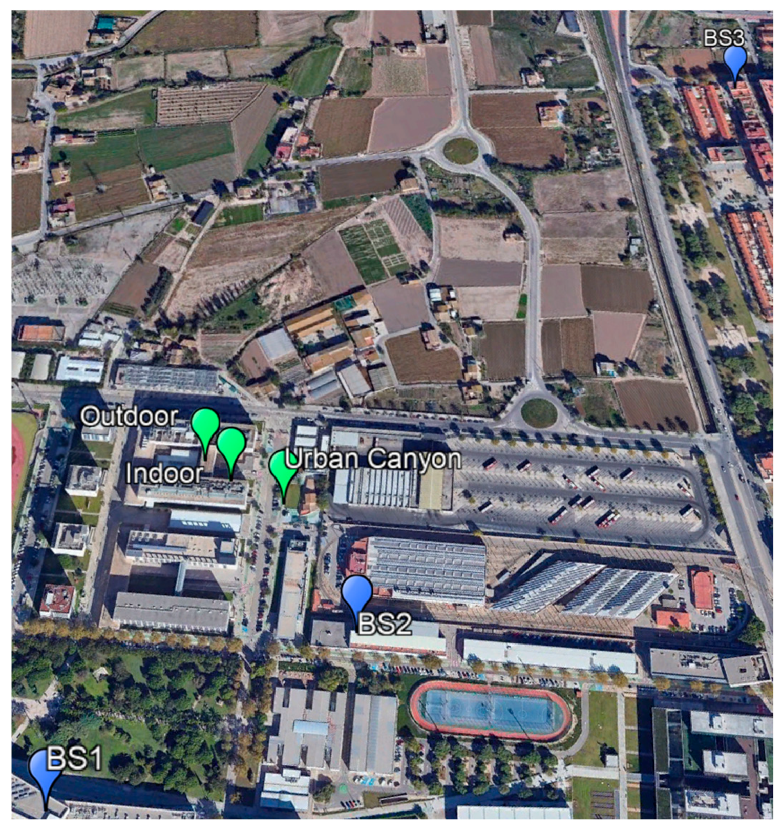
Funding

This research received no external funding.

Institutional Review Board Statement

Not applicable.

Informed Consent Statement

Not applicable.

Data Availability Statement

The raw data used in this study were submitted to Applied Sciences as Supplementary Materials and are available from the corresponding author upon reasonable request.

Conflicts of Interest

The authors declare no conflict of interest.

Appendix A

CellTracker is an Android application built on Google’s official Geolocation Application Programming Interface (API), designed to obtain the user’s location even when GPS is not available (Figure A1). It interacts with cell towers through HTTPS POST requests and receives a response in JSON format, containing the latitude, longitude, and estimated accuracy radius (Figure A2) [40].
Figure A1. Main interface of the CellTracker app.
Applsci 15 06300 g0a1
Figure A2. HTTPS POST request to the Geolocation API and response in JSON format.
Applsci 15 06300 g0a2
The app also displays extended mobile network information, including the BS ID, MNC, TAC, CI, and PCI; the available mobile network types, such as NR, LTE, GSM, and HSPA; and associated parameters like EARFCN, TA, RSRP, RSRQ, and RSSNR, as well as the downlink and uplink band frequencies. These data are extracted using Android’s telephony and location APIs, which provide access to telephony services and device connectivity information.
The availability of this information may vary depending on the mobile network operator, privacy policies, and the Android OS version installed on the device. CellTracker is publicly available for download.
The app exports observation data in .csv format, recording information about the interaction between the UE and nearby BSs. Each record includes fields such as the date, time, MCC, MNC, CI, LTE RSRP, network type, provider, Phone_Lat, Phone_Lon, and accuracy (m), among others, organized by the observation epoch. The provider column identifies the source of the location data: GPS refers to the phone’s GNSS sensor, network indicates a position provided by the mobile network, and WiFi refers to a position computed from nearby access points (if supported by the smartphone).

References

  1. Gill, S. How Many People Own Smartphones in the World? (2024–2029). Available online: https://prioridata.com/data/smartphone-stats/ (accessed on 15 May 2025).
  2. Resilient Societies. EUSPA EO and GNSS, Market Report; European Union Agency for the Space Programme (EUSPA): Luxembourg, 2024. [Google Scholar] [CrossRef]
  3. GSMA. The Mobile Economy 2025; GSM Association: London, UK, 2025; Available online: https://www.gsma.com/solutions-and-impact/connectivity-for-good/mobile-economy/wp-content/uploads/2025/02/030325-The-Mobile-Economy-2025.pdf (accessed on 1 April 2025).
  4. Federal Communications Commission (FCC). Available online: https://www.fcc.gov/ (accessed on 2 May 2025).
  5. 3GPP. Introducing 3GPP. Available online: https://www.3gpp.org/about-us/introducing-3gpp (accessed on 1 May 2025).
  6. FCC. FCC & Wireless Communications and Public Safety Act of 1999. Available online: https://www.congress.gov/bill/106th-congress/house-bill/438 (accessed on 1 February 2025).
  7. FCC. FCC Wireless E911 Location Accuracy Requirements, Fourth Report and Order. 2015. Available online: https://www.fcc.gov/document/fcc-adopts-new-wireless-indoor-e911-location-accuracy-requirements (accessed on 27 April 2025).
  8. 3GPP. 3GPP TS 23.271, Functional Stage 2 Description of Location Services (LCS), V9.4.0. 2010. Available online: https://portal.3gpp.org/desktopmodules/Specifications/SpecificationDetails.aspx?specificationId=834 (accessed on 15 May 2025).
  9. Dwivedi, S.; Shreevastav, R.; Munier, F.; Nygren, J.; Siomina, I.; Lyazidi, Y.; Shrestha, D.; Lindmark, G.; Ernström, P.; Stare, E.; et al. Positioning in 5G Networks. IEEE Commun. Mag. 2021, 59, 38–44. [Google Scholar] [CrossRef]
  10. 3GPP. TS 36.305 V17.1.0, LTE; Evolved Universal Terrestrial Radio Access Network (E-UTRAN); Stage 2 Functional Specification of User Equipment (UE) Positioning in E-UTRAN. 2022. Available online: https://www.etsi.org/deliver/etsi_ts/136300_136399/136305/17.01.00_60/ts_136305v170100p.pdf (accessed on 30 May 2025).
  11. García, A.C.; Maier, S.; Phillips, A. Location-Based Services in Cellular Networks: From GSM to 5G NR; Artech House: Boston, MA, USA, 2020. [Google Scholar]
  12. Groves, P.D. Principles of GNSS, Inertial, and Multisensor Integrated Navigation Systems, 2nd ed.; Artech House: Boston, MA, USA; London, UK, 2013. [Google Scholar]
  13. Del Peral-Rosado, J.A.; Estatuet i Castillo, R.; Mıguez-Sanchez, J.; Navarro-Gallardo, M.; García-Molina, J.A.; López-Salcedo, J.A.; Seco-Granados, G.; Zanier, F.; Crisci, M. Performance Analysis of Hybrid GNSS and LTE Localization in Urban Scenarios. In Proceedings of the 8th ESA Workshop on Satellite Navigation Technologies and European Workshop on GNSS Signals and Signal Processing (NAVITEC), Noordwijk, The Netherlands, 14–16 December 2016; pp. 1–8. [Google Scholar] [CrossRef]
  14. Alghisi, M.; Biagi, L. Positioning with GNSS and 5G: Analysis of Geometric Accuracy in Urban Scenarios. Sensors 2023, 23, 2181. [Google Scholar] [CrossRef] [PubMed]
  15. Gante, J.; Sousa, L.; Falcao, G. Dethroning GPS: Low-Power Accurate 5G Positioning Systems Using Machine Learning. IEEE J. Emerg. Sel. Top. Circuits Syst. 2020, 10, 240–252. [Google Scholar] [CrossRef]
  16. Del Peral-Rosado, J.A.; Saloranta, J.; Destino, G.; López-Salcedo, J.A.; Seco-Granados, G. Methodology for simulating 5G and GNSS high-accuracy positioning. Sensors 2018, 18, 3220. [Google Scholar] [CrossRef] [PubMed]
  17. Del Peral-Rosado, J.A.; Nolle, P.; Razavi, S.M.; Lindmark, G.; Shrestha, D.; Gunnarsson, F.; Kaltenberger, F.; Sirola, N.; Särkkä, O.; Roström, J.; et al. Design Considerations of Dedicated and Aerial 5G Networks for Enhanced Positioning Services. In Proceedings of the 10th Workshop on Satellite Navigation Technology, NAVITEC, Noordwijk, The Netherlands, 5–7 April 2022; Institute of Electrical and Electronics Engineers Inc.: Piscataway, NJ, USA, 2022. [Google Scholar] [CrossRef]
  18. Van Diggelen, F. A-GPS: Assisted GPS, GNSS, and SBAS; Artech: London, UK, 2009. [Google Scholar]
  19. Xhafa, A.; del Peral-Rosado, J.A.; López-Salcedo, J.A.; Seco-Granados, G. Evaluation of 5G Positioning Performance Based on UTDoA, AoA and Base-Station Selective Exclusion. Sensors 2022, 22, 101. [Google Scholar] [CrossRef] [PubMed]
  20. Liu, J.; Deng, Z.; Hu, E.; Huang, Y.; Deng, X.; Zhang, Z.; Ding, Z.; Liu, B. GNSS-5G Hybrid Positioning Based on Joint Estimation of Multiple Signals in a Highly Dependable Spatio-Temporal Network. Remote Sens. 2023, 15, 4220. [Google Scholar] [CrossRef]
  21. Duong, P.B.; Ghimire, B.; Dietmayer, K.; Ali, S.U.; Al Kim, H.; Seitz, J. Supervised Machine Learning Assisted Hybrid Positioning based on GNSS and 5G. In Proceedings of the 2022 IEEE 12th International Conference on Indoor Positioning and Indoor Navigation (IPIN), Beijing, China, 5–8 September 2022; pp. 1–8. [Google Scholar] [CrossRef]
  22. Gao, K.; Wang, H.; Lv, H.; Liu, W. Toward 5G NR High-Precision Indoor Positioning via Channel Frequency Response: A New Paradigm and Dataset Generation Method. IEEE J. Sel. Areas Commun. 2022, 40, 2233–2247. [Google Scholar] [CrossRef]
  23. Del Peral-Rosado, J.A.; Raulefs, R.; López-Salcedo, J.A.; Seco-Granados, G. Survey of Cellular Mobile Radio Localization Methods: From 1G to 5G. IEEE Commun. Surv. Tutor. 2018, 20, 1124–1148. [Google Scholar] [CrossRef]
  24. Feng, X.; Wang, K.; Liu, H.; Zhang, X.; Yang, S.H. An Adaptive IMU/UWB Fusion Method for NLOS Indoor Positioning and Navigation. IEEE Internet Things J. 2023, 10, 11414–11428. [Google Scholar] [CrossRef]
  25. Garraffa, G.; Ottavi, M.; Rinaldi, A.; Sangiovanni, V.; Trujillo, D.M. Localization Based on Parallel Robots Kinematics as an Alternative to Trilateration. IEEE Trans. Ind. Electron. 2022, 69, 718–728. [Google Scholar] [CrossRef]
  26. Horn, B.K.P. Celltracker. Available online: https://people.csail.mit.edu/bkph/CellTracker (accessed on 2 May 2025).
  27. Geo++. Geo++ RINEX Logger. Available online: https://www.geopp.de/ (accessed on 7 May 2025).
  28. Jiménez Martínez, M.; Quesada Olmo, N.; Villar Cano, M.; Paredes Asencio, J.; Marqués Mateu, A. Ajuste Gaussiano de Redes por el Método de Incrementos de Coordenadas. Valencia, Spain. 2011. Available online: http://www.racv.es/files/Ajuste_gaussiano_de_redes_metodo_incremento_coordenadas.pdf (accessed on 7 May 2025).
  29. Berné Valero, J.L.; Garrido Villén, N.; Capilla Roma, R. GNSS: Geodesia Espacial y Geomática; Editorial Universitat Politècnica de València: Valencia, Spain, 2023. [Google Scholar]
  30. Ghilani, C.D.; Wolf, P.R. Adjustment Computations: Spatial Data Analysis; John Wiley & Sons: Hoboken, NJ, USA, 2006. [Google Scholar]
  31. Strang, G.; Borre, K. Linear Algebra, Geodesy, and GPS; Wellesley-Cambridge Press: Wellesley, MA, USA, 1997. [Google Scholar]
  32. Leick, A.; Rapoport, L.; Tatarnikov, D. GPS Satellite Surveying, 4th ed.; John Wiley & Sons: Hoboken, NJ, USA, 2015. [Google Scholar]
  33. Xu, G.; Xu, Y. GPS: Theory, Algorithms and Applications, 3rd ed.; Springer: Berlin/Heidelberg, Germany, 2016. [Google Scholar] [CrossRef]
  34. Sanz Subirana, J.; Hernandez-Pajares, M.; Juan Zornoza, J.M. GNSS Data Processing: Fundamentals and Algorithms; ESA Communications: Noordwijk, The Netherlands, 2013; Volume I. [Google Scholar]
  35. Gobierno de España; Ministerio para la Transformación Digital y de la Función Pública; Secretaría de Estado para la Sociedad de la Información y la Agenda Digital. Infoantenas. Available online: https://geoportal.minetur.gob.es/VCTEL/vcne.do (accessed on 28 March 2025).
  36. Li, B.; Harvey, B.; Gallagher, T. Using Barometers to Determine the Height for Indoor Positioning. In Proceedings of the International Conference on Indoor Positioning and Indoor Navigation (IPIN), Montbéliard, France, 28–31 October 2013. [Google Scholar]
  37. Sun, Z.; Gao, W.; Tao, X.; Pan, S.; Wu, P.; Huang, H. Semi-Tightly Coupled Robust Model for GNSS/UWB/INS Integrated Positioning in Challenging Environments. Remote Sens. 2024, 16, 2108. [Google Scholar] [CrossRef]
  38. Zhang, F.; Li, J.; Zhang, X.; Duan, S.; Yang, S.-H. Indoor Fusion Positioning Based on “IMU-Ultrasonic-UWB” and Factor Graph Optimization Method. arXiv 2025, arXiv:2503.12726. [Google Scholar]
  39. Schwarzbach, P.; Michler, A.; Michler, O. Grid-Based Hybrid 3DMA GNSS and Terrestrial Positioning. arXiv 2023, arXiv:2309.05644. [Google Scholar]
  40. Google Maps Platform. Geolocation API Overview. Available online: https://developers.google.com/maps/documentation/geolocation/overview?hl=es-419 (accessed on 26 March 2025).
Figure 1. Geographic positions of the BSs and UE locations for the outdoor, indoor, and urban canyon scenarios.
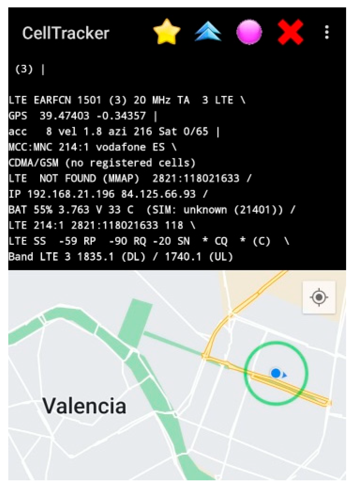
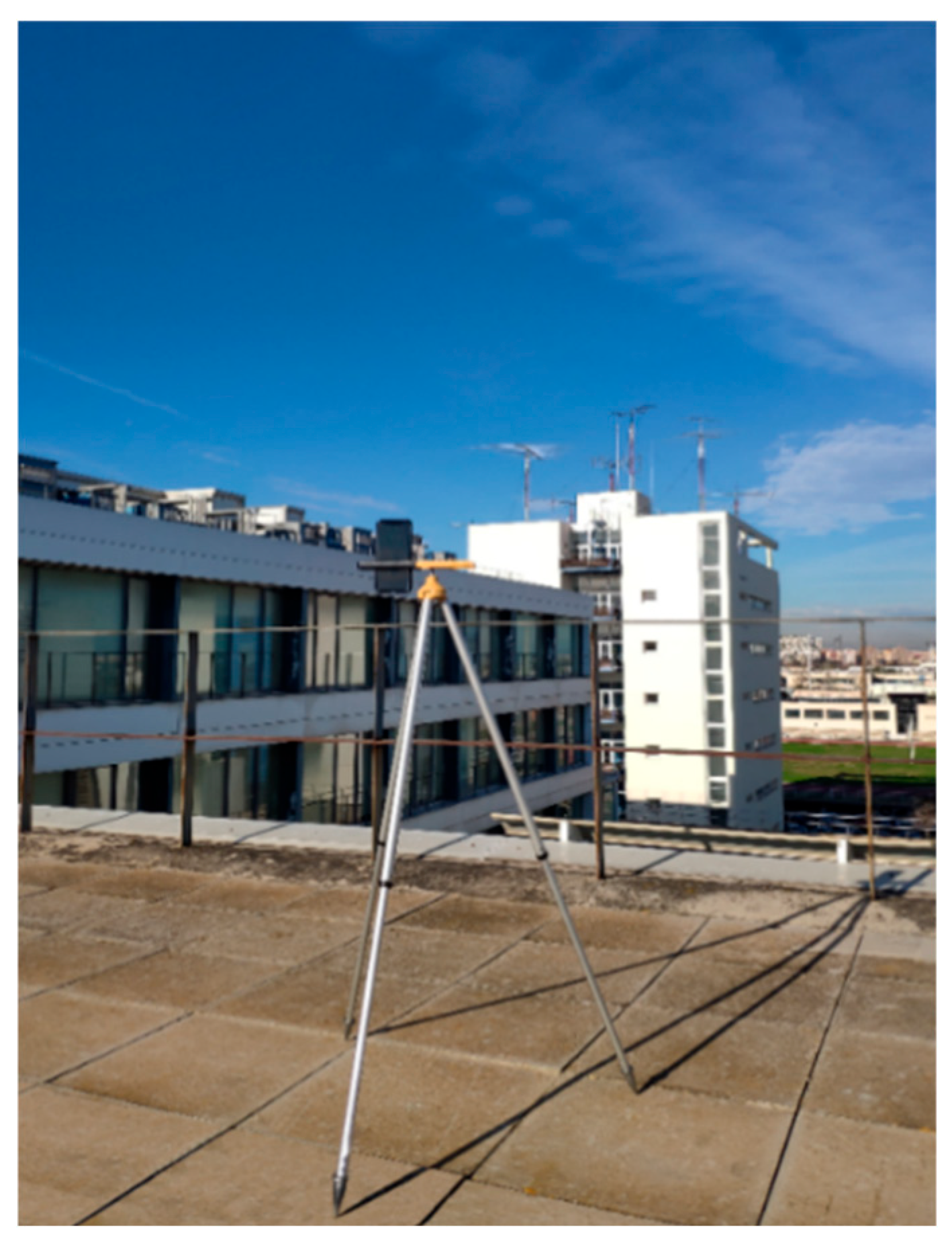
Applsci 15 06300 g001
Figure 2. UE—Xiaomi Mi 8 Pro smartphone—positioned on a rooftop in the outdoor scenario.
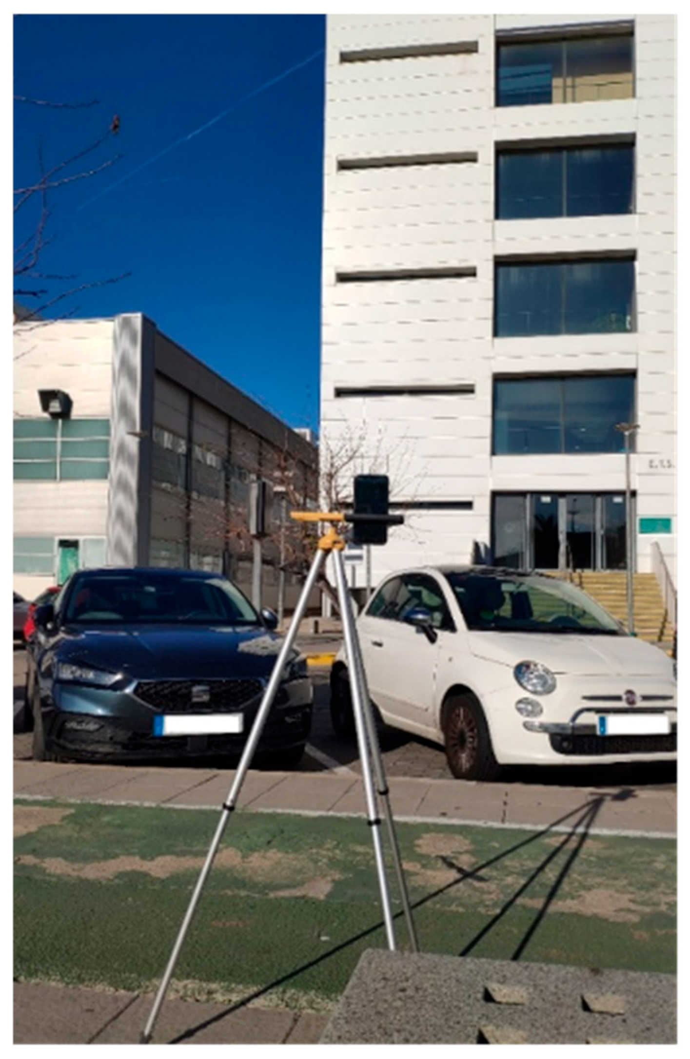
Applsci 15 06300 g002
Figure 3. UE—Xiaomi Mi 8 Pro smartphone —in the urban canyon scenario.
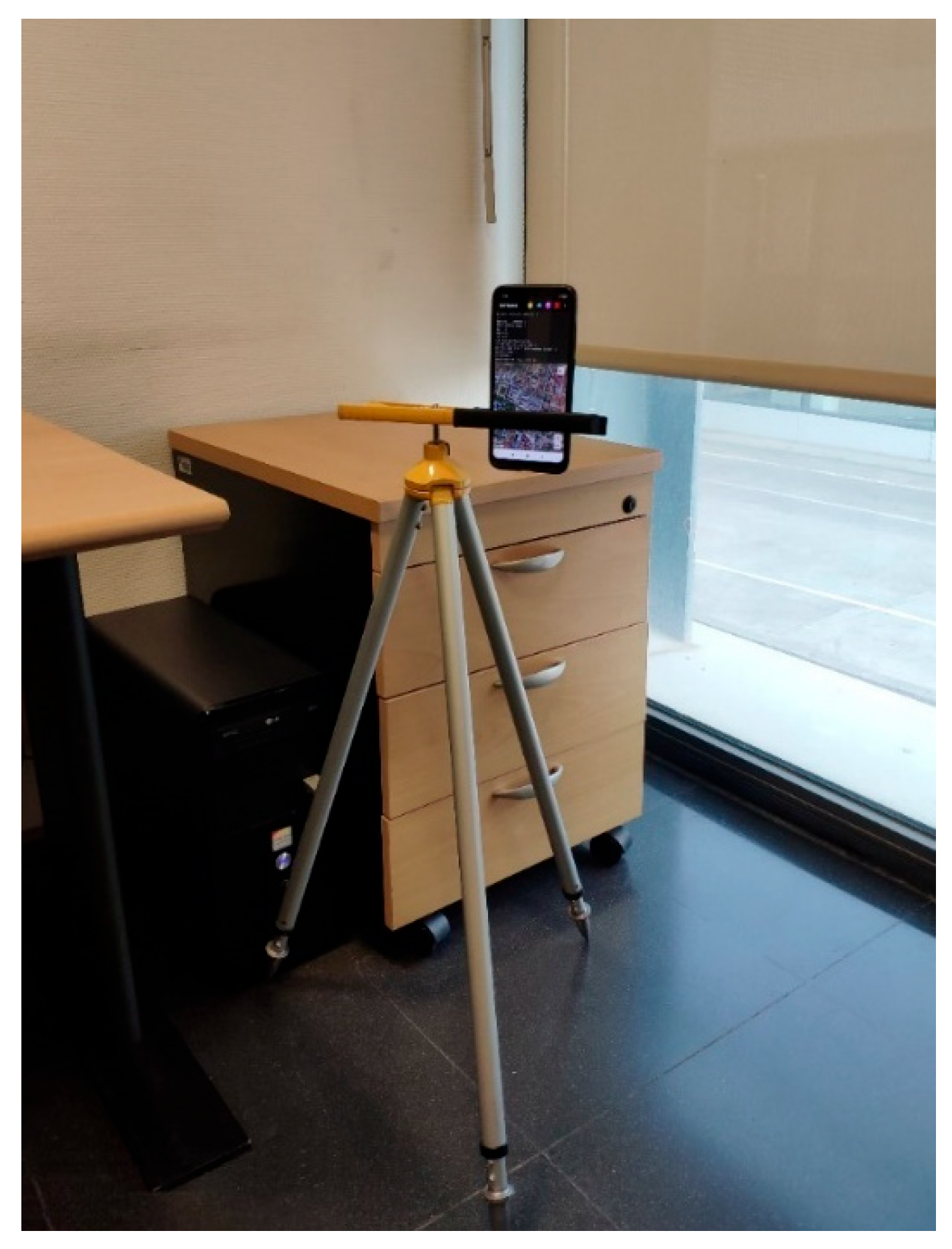
Applsci 15 06300 g003
Figure 4. UE—Xiaomi Mi 8 Pro smartphone—positioned near a window in the indoor scenario.
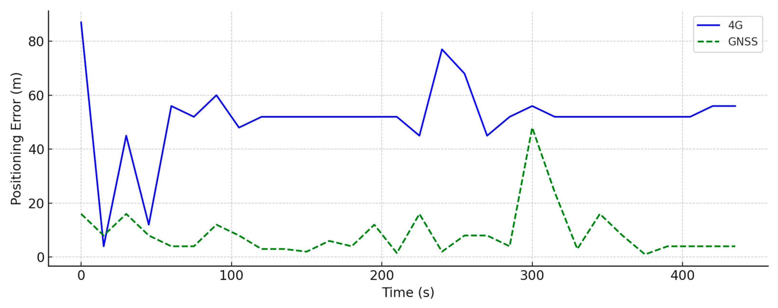
Applsci 15 06300 g004
Figure 5. Time series of a priori positioning errors in the outdoor scenario using GNSS and 4G data collected at 15 s intervals. GNSS demonstrated a stable and low-error performance under open-sky conditions, while 4G showed more variability and a less consistent accuracy.
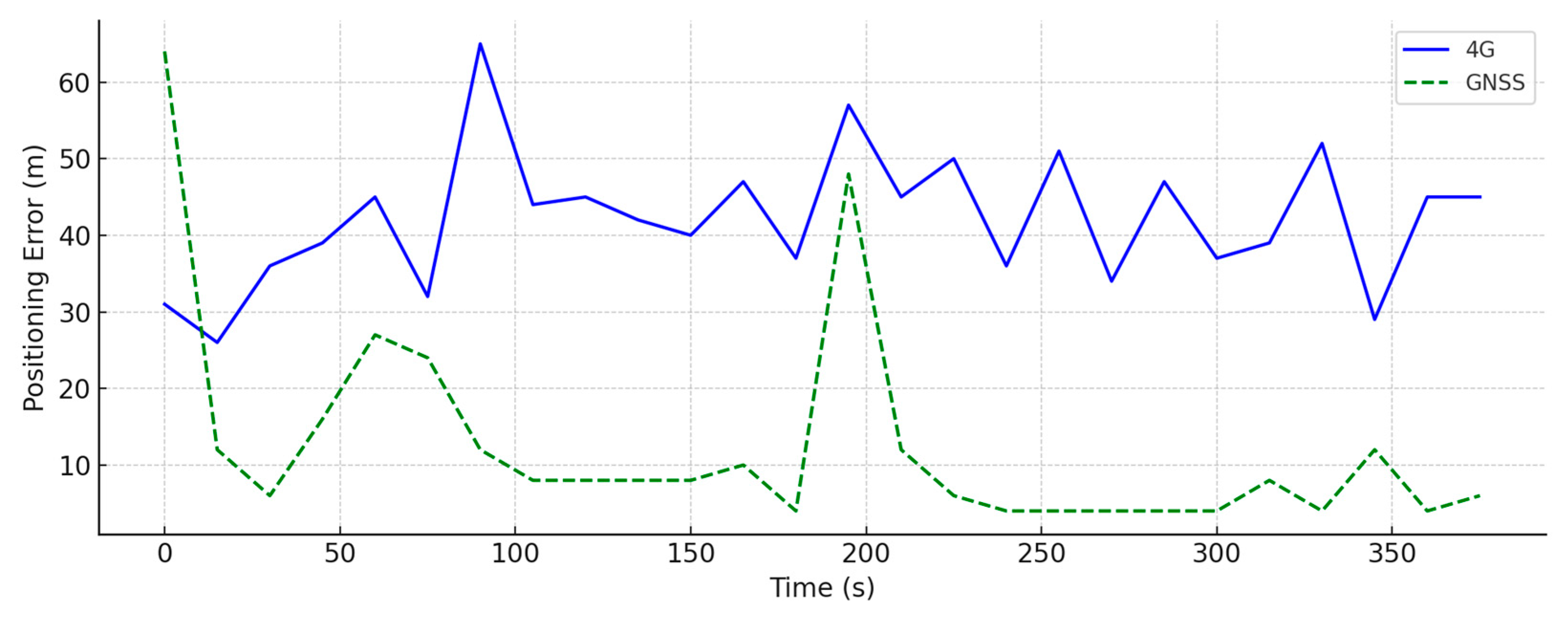
Applsci 15 06300 g005
Figure 6. Time series of a priori positioning errors in the urban canyon scenario using GNSS and 4G data. Sampling was performed every 15 s. GNSS showed moderate fluctuations, while 4G exhibited a pronounced instability due to multipath and partial obstruction in the environment.
Applsci 15 06300 g006
Figure 7. Time series of a priori positioning errors in the indoor scenario using GNSS and 4G data. Data were collected at 15 s intervals. GNSS performance showed greater variability due to signal degradation in enclosed environments, while 4G offered a comparatively more stable accuracy.
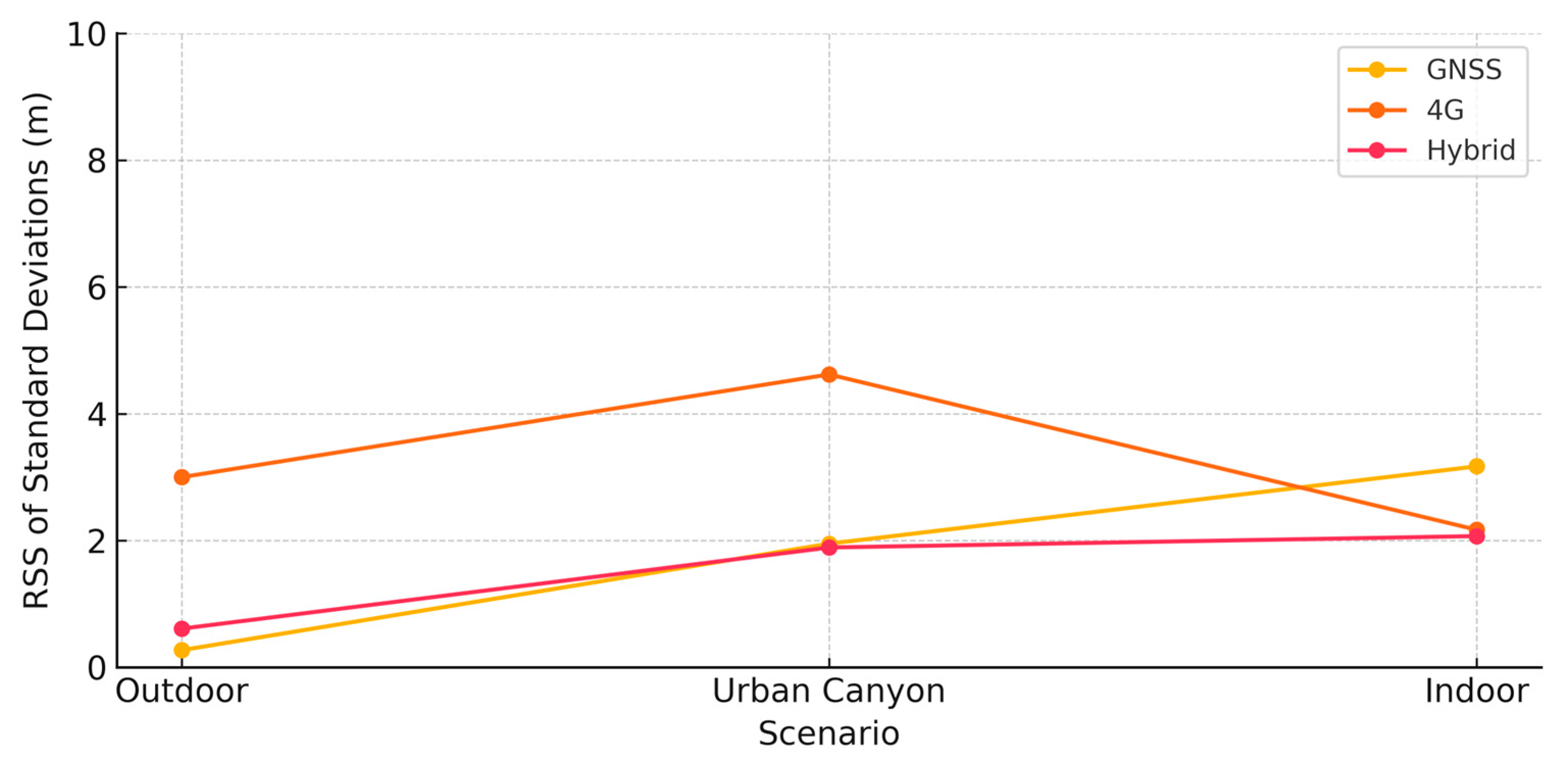
Applsci 15 06300 g007
Figure 8. Root sum square (RSS) of standard deviations for the position-level method across the outdoor, urban canyon, and indoor scenarios. This metric reflects the internal precision of the GNSS-only, 4G-only, and hybrid solutions.
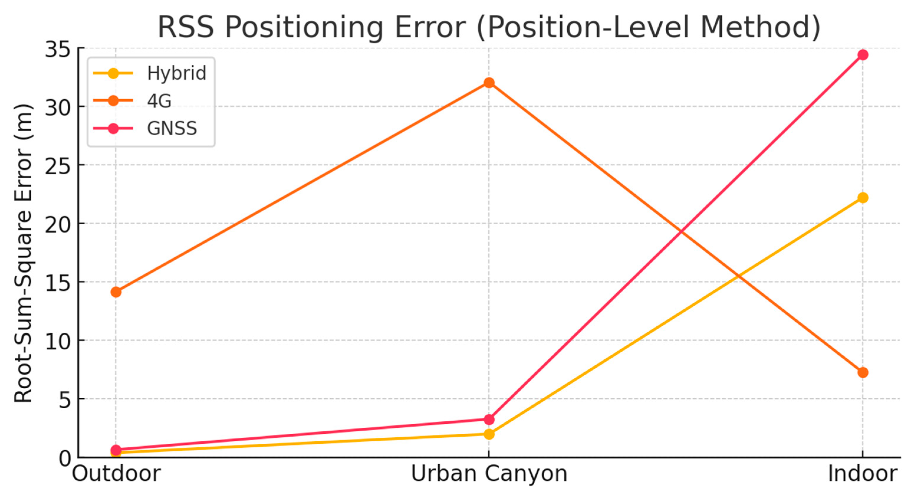
Applsci 15 06300 g008
Figure 9. Root sum square (RSS) of positioning errors for the position-level hybridization method across the outdoor, urban canyon, and indoor scenarios. This graph summarizes the overall accuracy achieved by each solution in the three test environments.
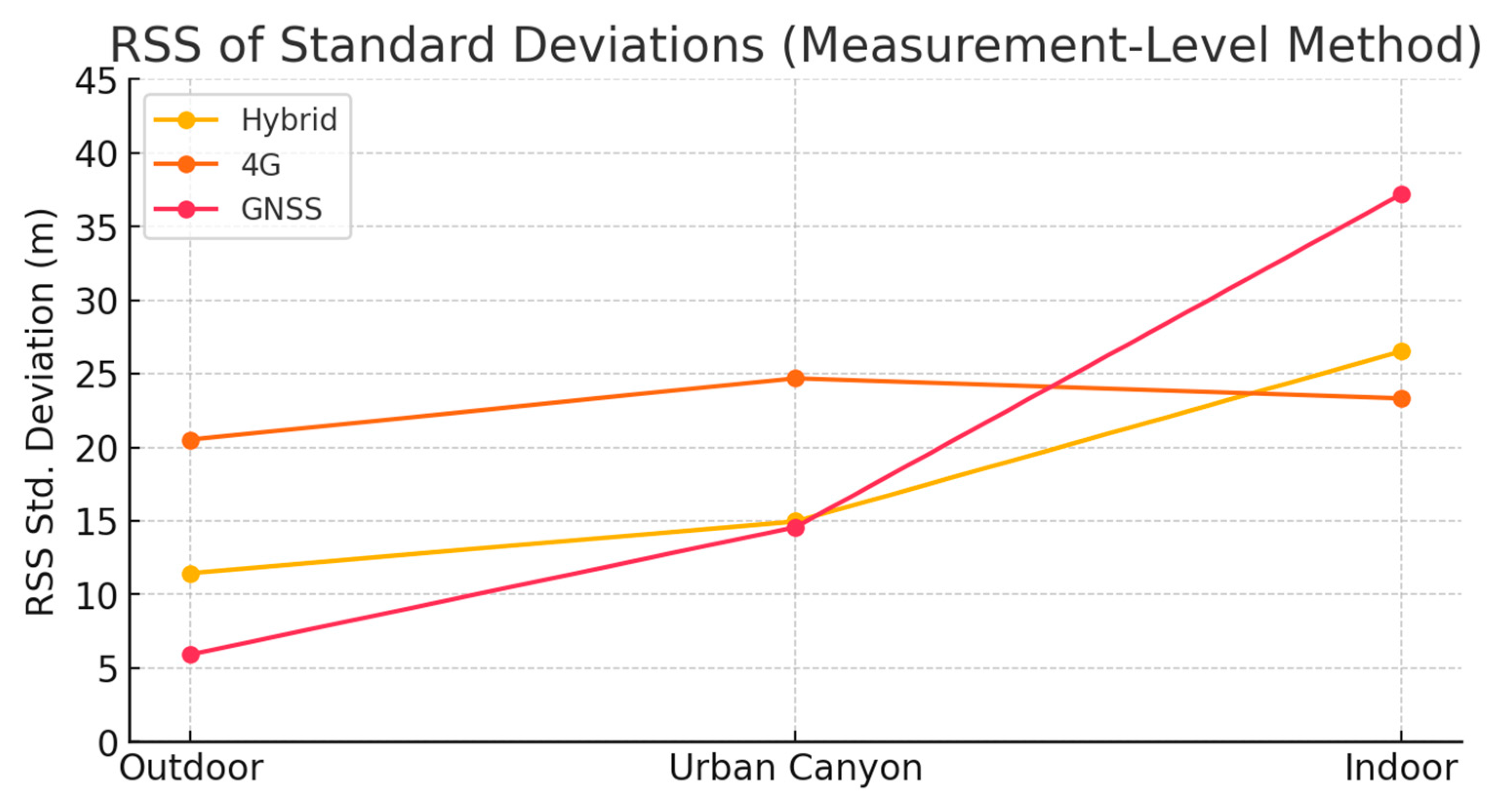
Applsci 15 06300 g009
Figure 10. Root sum square (RSS) of standard deviations for the measurement-level hybridization method across the outdoor, urban canyon, and indoor scenarios. This metric quantifies the internal precision of each method tested.
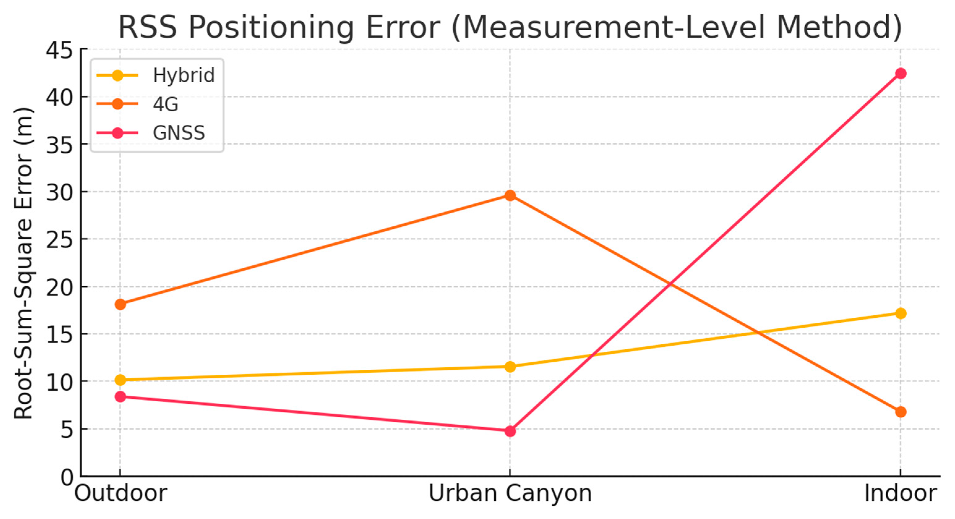
Applsci 15 06300 g010
Figure 11. Root sum square (RSS) of positioning errors with respect to the reference coordinates for the measurement-level hybridization method. This graph summarizes the total positioning accuracy for each solution in the three test environments.
Applsci 15 06300 g011
Table 1. BS coordinates and associated standard deviations.
BSE (m)N (m)U (m) σ E (m) σ N (m) σ U (m)
BS1728,856.174,373,346.2093.220.030.020.04
BS2729,094.424,373,423.4372.070.010.030.05
BS3729,592.054,373,891.1482.220.020.020.05
Table 2. Reference point coordinates and associated standard deviations.
ScenariosE (m)N (m)U (m) σ E (m) σ N (m) σ U (m)
Outdoor729,010.114,373,590.0672.980.030.020.04
Urban canyon729,063.614,373,540.1755.070.010.030.05
Indoor729,034.204,373,567.7660.580.020.020.05
Table 3. Root mean square (RMS) positioning errors computed from the raw field data corresponding to Figure 5, Figure 6 and Figure 7. The values quantify the positioning performance of GNSS and 4G across the three experimental scenarios: indoor, urban canyon, and outdoor. These are a priori errors as directly reported by the UE, prior to applying any hybridization methods or outlier suppression techniques.
Data CollectedGNSS RMS (m) 4G RMS (m)
Indoor 27.8120.87
Urban canyon18.8043.03
Outdoor12.6253.56
Table 4. Estimated coordinates and standard deviations for the outdoor scenario using the hybrid, GNSS-only, and 4G-only solutions. The RSS column reports the root sum square of the standard deviations for the east, north, and up components, providing a compact measure of internal precision.
ObsE (m)N (m)U (m) σ E (m) σ N (m) σ U (m)RSS
Hybrid729,009.804,373,590.0273.220.340.490.110.61
4G729,006.454,373,576.4072.392.241.970.353.00
GNSS729,009.634,373,590.2072.540.040.170.210.27
Table 5. Estimated coordinates and standard deviations for the urban canyon scenario using the hybrid, GNSS-only, and 4G-only solutions. The RSS column indicates the combined 3D precision via the root sum square of standard deviations for the three spatial axes.
ObsE (m)N (m)U (m) σ E (m) σ N (m) σ U (m)RSS
Hybrid729,061.974,373,539.5457.041.331.200.591.89
4G729,034.674,373,539.7057.262.304.010.124.62
GNSS729,065.844,373,538.4457.700.580.901.631.95
Table 6. Estimated coordinates and standard deviations for the indoor scenario using the hybrid, GNSS-only, and 4G-only solutions. The RSS column reflects the total standard deviation across the east, north, and up components.
ObsE (m)N (m)U (m) σ E (m) σ N (m) σ U (m)RSS
Hybrid729,037.884,373,589.1264.991.191.221.172.07
4G729,031.994,373,574.2660.201.781.010.732.17
GNSS729,042.294,373,598.9872.291.221.982.163.17
Table 7. Accuracy comparison of the hybrid, GNSS-only, and 4G-only solutions in the outdoor environment. The RSS column summarizes the total positioning error relative to the reference coordinates, computed as the root sum square of the east, north, and up errors.
Obs d E (m) d N (m) d U (m)RSS
Hybrid0.310.04−0.240.39
4G3.6513.660.5814.15
GNSS0.48−0.130.430.66
Table 8. Accuracy comparison of the hybrid, GNSS-only, and 4G-only solutions in the urban canyon environment. The RSS column provides the total 3D positioning error using the root sum square of the individual component errors.
Obs d E (m) d N (m) d U (m)RSS
Hybrid1.640.62−0.962.00
4G28.93−13.80−1.2032.08
GNSS−2.251.73−1.633.27
Table 9. Accuracy comparison of the hybrid, GNSS-only, and 4G-only solutions in the indoor environment. The RSS column indicates the combined positioning error in three dimensions based on the root sum square calculation.
Obs d E (m) d N (m) d U (m)RSS
Hybrid−3.68−21.36−4.8422.21
4G2.65−6.75−0.517.27
GNSS−8.00−31.22−12.1434.44
Table 10. Estimated coordinates and standard deviations for the outdoor scenario using the hybrid, GNSS-only, and 4G-only solutions. The RSS column summarizes the standard deviations for all three components using the root sum square metric.
ObsE (m)N (m)U (m) σ E (m) σ N (m) σ U (m)RSS
Hybrid729,010.464,373,589.6962.841.802.0111.1311.45
4G729,008.604,373,588.0354.992.430.8320.3520.51
GNSS729,011.234,373,591.4564.771.273.704.445.92
Table 11. Estimated coordinates and standard deviations for the urban canyon scenario using the hybrid, GNSS-only, and 4G-only solutions. The RSS column expresses the overall precision via the root sum square of the component-wise standard deviations.
ObsE (m)N (m)U (m) σ E (m) σ N (m) σ U (m)RSS
Hybrid729,055.514,373,547.9357.885.054.7813.2514.96
4G729,037.964,373,554.2259.734.260.2924.3224.69
GNSS729,064.294,373,544.7953.965.954.6212.4814.58
Table 12. Estimated coordinates and standard deviations for the indoor scenario using the hybrid, GNSS-only, and 4G-only solutions. The RSS column shows the total internal dispersion calculated from the standard deviations for E, N, and U.
ObsE (m)N (m)U (m) σ E (m) σ N (m) σ U (m)RSS
Hybrid729,041.094,373,576.0573.965.0612.0623.0626.51
4G729,038.714,373,562.7859.38 4.810.5122.8023.31
GNSS729,046.504,373,599.3386.2217.7521.3524.7337.18
Table 13. Accuracy comparison of the hybrid, GNSS-only, and 4G-only solutions in the outdoor environment. The RSS column presents the total positioning error using the root sum square of the E, N, and U errors.
Obs d E (m) d N (m) d U (m)RSS
Hybrid−0.350.3710.1410.15
4G1.512.0317.9818.16
GNSS−1.12−1.398.218.40
Table 14. Accuracy comparison of the hybrid, GNSS-only, and 4G-only solutions in the urban canyon environment. The RSS column quantifies the overall 3D positioning error using the root sum square method.
Obs d E (m) d N (m) d U (m)RSS
Hybrid8.10−7.76−2.8111.56
4G25.65−14.05−4.6629.61
GNSS−0.68−4.621.114.80
Table 15. Accuracy comparison of the hybrid, GNSS-only, and 4G-only solutions in the indoor environment. The RSS column contains the root sum square of the positional error components, offering a single accuracy metric.
Obs d E (m) d N (m) d U (m)RSS
Hybrid−6.89−8.29−13.3917.19
4G−4.514.981.206.82
GNSS−12.30−31.57−25.6442.49
Table 16. Overall performance of hybrid, GNSS, and 4G positioning methods in outdoor, urban canyon, and indoor scenarios.
Method σ E (m) σ N (m) σ U (m)
OutdoorMeasurement level1.27 (GNSS)3.70 (GNSS)4.44 (GNSS)
Position level 0.04 (GNSS)0.17 (GNSS)0.11(Hybrid)
IndoorMeasurement level4.81 (4G)0.51 (4G)22.80 (4G)
Position level1.19 (Hybrid)1.22 (Hybrid)0.73 (4G)
Urban canyonMeasurement level5.95 (GNSS)4.62 (GNSS)12.48 (GNSS)
Position level0.58 (GNSS)0.90 (GNSS)0.12 (4G)
Disclaimer/Publisher’s Note: The statements, opinions and data contained in all publications are solely those of the individual author(s) and contributor(s) and not of MDPI and/or the editor(s). MDPI and/or the editor(s) disclaim responsibility for any injury to people or property resulting from any ideas, methods, instructions or products referred to in the content.

