Gaussian-UDSR: Real-Time Unbounded Dynamic Scene Reconstruction with 3D Gaussian Splatting

Abstract

Unbounded dynamic scene reconstruction is crucial for applications such as autonomous driving, robotics, and virtual reality. However, existing methods struggle to reconstruct dynamic scenes in unbounded outdoor environments due to challenges such as lighting variation, object motion, and sensor limitations, leading to inaccurate geometry and low rendering fidelity. In this paper, we proposed Gaussian-UDSR, a novel 3D Gaussian-based representation that efficiently reconstructs and renders high-quality, unbounded dynamic scenes in real time. Our approach fused LiDAR point clouds and Structure-from-Motion (SfM) point clouds obtained from an RGB camera, significantly improving depth estimation and geometric accuracy. To address dynamic appearance variations, we introduced a Gaussian color feature prediction network, which adaptively captures global and local feature information, enabling robust rendering under changing lighting conditions. Additionally, a pose-tracking mechanism ensured precise motion estimation for dynamic objects, enhancing realism and consistency. We evaluated Gaussian-UDSR on the Waymo and KITTI datasets, demonstrating state-of-the-art rendering quality with an 8.8% improvement in PSNR, a 75% reduction in LPIPS, and a fourfold speed improvement over existing methods. Our approach enables efficient, high-fidelity 3D reconstruction and fast real-time rendering of large-scale dynamic environments, while significantly reducing model storage overhead.

1. Introduction

Boundless dynamic scene reconstruction is crucial in autonomous driving, high-precision mapping, and virtual reality. For example, by reconstructing dynamic environments, autonomous driving systems can more accurately understand the structure and composition of their surroundings and distinguish between static objects and dynamic objects to make more effective path planning and decision-making. These capabilities require us to reconstruct 3D scenes from captured environmental information efficiently and render high-quality novel views in real time, which remains a challenge in unbounded dynamic environments.

Scene representations based on Neural Radiance Fields [1,2,3,4,5,6,7], among others, have been extensively explored in the existing literature. S-NeRF [4] improves 3D reconstruction in street view with an optimized network structure. However, it is sensitive to low-quality images and illumination variations, leading to possible errors in the 3D models generated in complex environments. Streetsurf [5] applies a multi-view implicit surface reconstruction technique to street view to generate accurate 3D reconstruction by extending it to street view while dealing with the complexity of moving objects and dynamic environments. However, the accuracy may be limited due to the low quality of street-view images and the influence of complex illumination and occlusion. There may be computational efficiency problems for the processing of unbounded scenes, and there still needs improvement in the processing of dynamic objects, especially in real time. Moreover, this is a crucial aspect in simulating autonomous driving environments.

Recently, several approaches [8,9,10,11] propose to represent a dynamic scene as a synthetic neural representation consisting of a moving car in the foreground and a static background. The NSG [9] approach learns the object and motion relationships in the scene graph through neural networks, encodes spatial relationships between different objects, and efficiently supports the modeling and tracking of dynamic objects, which is not only able to perform dynamic scene modeling, but also capture the interactions between objects. interactions. However, the problem of computational complexity is still faced in unbounded and complex scenes, and the graph structure may lead to time and space efficiency problems. Panoptic Neural Fields (PNF) [10], which combines semantic segmentation with a neural field representation, enables the model to understand and generate scenes containing multiple semantic objects. By layering the objects in the scene, PNF provides better object-background separation, leading to more accurate modeling of dynamic and static objects. Despite providing better modeling for static objects, PNF still has limited performance for dynamic objects in the scene, especially fast-moving objects.

In this work, we propose Gaussian-UDSR, a novel representation framework designed to tackle the core challenge of real-time reconstruction and rendering of unbounded dynamic scenes, which is essential for autonomous driving and other large-scale dynamic environments. Our key idea is to adopt 3D Gaussian splatting as a unified representation to jointly model static backgrounds and dynamic foreground objects. This representation is lightweight, differentiable, and well-suited for real-time processing. It also integrates LiDAR and SfM point cloud data, leveraging the precise geometry from LiDAR and dense texture information from SfM, thus enhancing scene reconstruction quality in unbounded outdoor environments.

Our second contribution is the introduction of a Gaussian feature prediction network, which replaces traditional spherical harmonic basis functions with a learnable module. This network effectively captures both global contextual information and local object-specific features, enabling robust appearance modeling under varying lighting conditions and occlusions.

Finally, we conduct comprehensive experiments on the Waymo and KITTI datasets. The results demonstrate that our method significantly outperforms existing state-of-the-art approaches in terms of both rendering quality and speed, validating its practical effectiveness in real-world autonomous driving scenarios [9,12].

2. Related Work

Novel view synthesis is a crucial technique in computer vision and autonomous driving. In recent years, some works [13,14,15,16,17,18] have reconstructed objects from multi-view images and LiDAR inputs. However, these methods are limited to existing images, cannot present new views, and need help processing high-resolution images, which usually produce a noisy appearance.

Neural Radiance Fields (NeRF) [19] has emerged as an approach of interest. NeRF employs coordinate-based multilayer perception of a 3D scene to predict the optical properties of the point in the scene and utilizes volume rendering and spatial smoothing of multilayer perception to generate high-quality novel views. However, its implicit nature also brings drawbacks, including slow training and rendering speeds and high memory consumption limited to simplified material and lighting models. Several studies have proposed solutions to these challenges to increase the training speed. Many NeRF-based methods [20,21,22,23,24] have achieved expressive compositing quality and good view consistency [25,26,27,28,29,30]. Instant-NGP [21] introduces multiresolution hash coding, allowing smaller networks to reduce training costs. Depth-supervised NeRF [25] utilizes depth maps for fast training with few viewpoints. Sparsenerf [30] improves the ability to synthesize new viewpoints from sparse viewpoint data by ordering the depth of information.

Recently, 3D Gaussian splatting for real-time radiance field rendering (3DGS) [31] has brought about a technological change by fundamentally addressing these pain points of NeRF. 3DGS expresses the scene as a displayed point cloud, retaining the high-quality benefits of volume rendering through a highly parallelized differentiable rasterization pipeline while significantly improving the training speed and rendering efficiency and providing control over the scene. However, 3DGS targets static scenes and cannot model dynamic moving objects. Therefore, some researchers have tried to introduce 3DGS techniques into the reconstruction of dynamic scenes 4DGS [32] and Control4D [33] encode the spatial features of the scene using Tri-Plane [34] and HexPlane [35], respectively, and decode them using multilayer perceptron (MLP) to obtain the motion changes of each Gaussian point. D3DGS [36] and GauFRe [37] directly utilize an unbounded MLP to predict the motion of each Gaussian point, and GauFRe also separates the Gaussian points statically and dynamically to distinguish between the static and dynamic parts of the field. SC-GS [38] introduces a set of control points to the scene and utilizes the MLP to predict the variation field of each control point. After that, the K-nearest neighbor (KNN) algorithm is used to find the neighboring control points of each Gaussian point and interpolate the neighboring control points’ variation field to obtain the Gaussian point’s motion variation. However, they are models constructed on small-scale data with low image quality and rendering speed. Therefore, this paper proposes a new 3D Gaussian framework-based unbounded dynamic scene reconstruction method, Gaussian-UDSR, for large-scale unbounded dynamic scenes focused on self-driving cars.

Table 1. Comparison of dynamic scene reconstruction methods.

Method	Input Modality	Scene Scale	Dynamic Modeling	Rendering Speed	Rendering Quality
D-NeRF [25]	RGB	Bounded (small)	MLP-based	Slow	Medium
4DGS [32]	RGB + TriPlane	Bounded (small)	plane features	Medium	High
SC-GS [38]	RGB + Control Points	Bounded (small)	control points + KNN	Medium	Medium
GauFRe [37]	RGB + MLP	Bounded (small)	separated Gaussians	Medium	High
Ours	LiDAR + RGB + MLP	Unbounded (large)	motion separation	Real time (Fast)	High

summarizes the representative dynamic scene reconstruction approaches based on NeRF and 3DGS, comparing them across input modality, scene scale, dynamic modeling capability, rendering speed, and quality. While methods like SC-GS and GauFRe show promise in small-scale scenes, they are limited in rendering resolution and real-time applicability. In contrast, our proposed Gaussian-UDSR targets large-scale unbounded dynamic scenes with improved motion separation and real-time rendering, tailored for autonomous driving scenarios.

3. Method

This section provides a comprehensive introduction to Gaussian-UDSR, a model for unbounded dynamic scene reconstruction that allows for fast reconstruction and real-time rendering. The lack of high-frequency and localized detailed information, the inefficiency of rendering, and the accuracy of vehicle pose tracking in the aforementioned NeRF-based approaches are addressed. In Section 3.1, we first present the complete framework of Gaussian-UDSR. Continuing Section 3.2, we introduce the Gaussian model, dividing it into static background and dynamic object models. The basic principle of projecting Gaussian ellipsoid in 3D space to 2D pixel plane to realize 3D scene reconstruction is also explained. Section 3.3 introduces the Gaussian color feature prediction network and delves into the dynamic feature sampler that focuses on global and local dynamic feature information. This network replaces the role of the original spherical harmonic function and aims at accurate prediction of color properties of dynamic 3D Gaussians. Finally, in Section 3.4, we present the loss function.

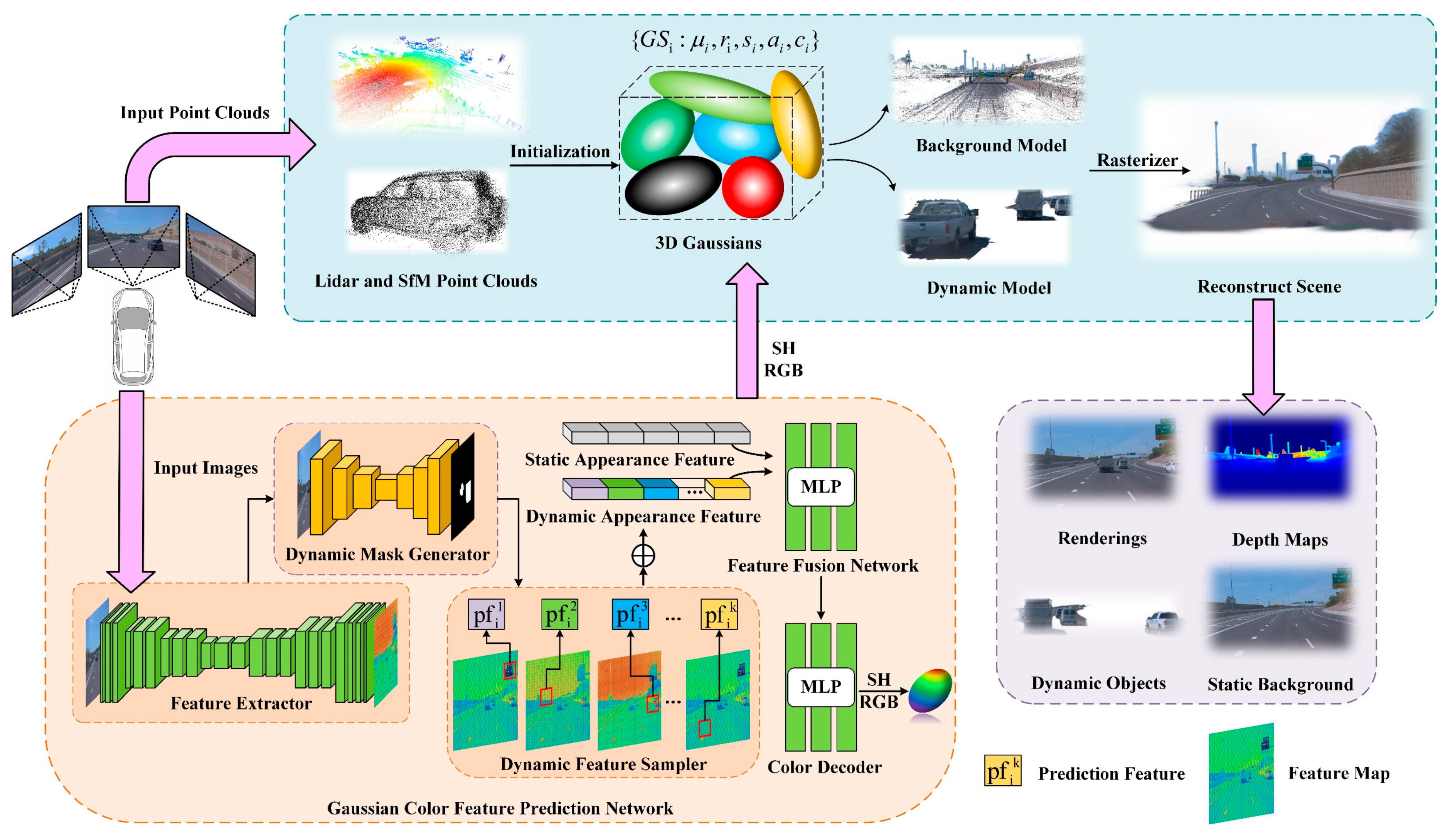
3.1. Overall Architecture

Our proposed method is shown in Figure 1. A microscopic rasterizer renders the scene after the static background and dynamic object models by parallel processing the LIDAR and camera data inputs in two channels. Firstly, the first channel transforms the camera-acquired image into a point cloud in 3D space by the SfM algorithm and fuses it with the sparse point cloud acquired by LIDAR to generate a dense point cloud, which is initialized as a primitive 3D Gaussian sphere. Meanwhile, the second channel takes the camera-acquired images for feature extraction, dynamically samples each feature map slice through a dynamic feature sampler, splices the sampled predicted features and fuses them with static appearance features using a feature fusion network, and then obtains Gaussian point color attributes under a specific viewing direction through a color decoding network. Finally, the Gaussian points of the two channels are jointly passed into the static background model and the dynamic object model, which are rendered by a fast micronize rasterizer.

3.2. Gaussian Model

The basic principle of Gaussian splatting is shown in Figure 2, where we initialize the SfM point cloud and the LiDAR point cloud as a cluster of Gaussian ellipsoids in 3D space and classify them into static background models and dynamic object models. All the Gaussian ellipsoids jointly affect the pixels on the corresponding raster, and a large number of ellipsoids perform a throwing process directly to the view plane, which leads to fast and high-quality rendering and building of complex scenes.

Static background model. The static background model is represented as a set of three-dimensional Gaussian points in the world coordinate system, and the covariance matrix ${\mathrm{\Sigma }}_s\in R^{3\times 3}$, the positional mean ${\mu }_s\in R^3$, the opacity ${\alpha }_s$, and the color $c_s$ jointly influence its shape expression:

$$G_s\left(x\right)=e^{-{\displaystyle \frac{1}{2}}{\left(x-{\mu }_s\right)}^T{{\mathrm{\Sigma }}_s}^{-1}\left(x-{\mu }_s\right)}$$

(1)

Meanwhile, the covariance matrix ${\mathrm{\Sigma }}_s$ can be decomposed into scaling matrix $S_s$ and rotation matrix $R_s$, where $S_s$ is represented by diagonal elements and $R_s$ is represented by unit quaternion. Quaternions are a compact and numerically stable representation of 3D rotations, defined by a four-dimensional vector ($q_w$, $q_x$, $q_y$, $q_z$) subject to the unit norm constraint. Compared to Euler angles, quaternions avoid gimbal lock and provide smooth interpolation (e.g., via SLERP), which is crucial for continuous pose tracking in dynamic scenes. Moreover, quaternions are more efficient and numerically stable than rotation matrices, as they require fewer parameters and avoid the need for orthonormalization. These advantages make quaternions particularly suitable for representing and optimizing camera and object orientations in our dynamic scene reconstruction framework. As shown in Figure 3, the unit sphere in the left figure is transformed into the ellipsoid in the right figure, and Equation (2) describes this transformation process. The rotation matrix $R_S$ changes the orientation of the unit sphere, while the scaling matrix $S_S$ scales it. Through rotation and scaling operations, the originally isotropic unit sphere is transformed into an anisotropic ellipsoid, which can more flexibly describe the multivariate correlations in complex environments. The covariance matrix ${\mathrm{\Sigma }}_s$ can be expressed as

$${\mathrm{\Sigma }}_s=R_s{S}_s{S}_s^T{R}_s^T$$

(2)

In addition to this, the rendering needs to project each Gaussian ellipsoid from the 3D space to the 2D view plane in order to obtain the image in the specified view direction, and the process of changing the projection is a nonlinear approximation, which can be expressed as a local linear approximation of the multivariate function at a point by the Jacobian matrix $J$. As shown in Figure 4, the Jacobian matrix $J$ (Equation (3)) in the projection model characterizes the local linear transformation relationship from 3D spatial coordinates to a 2D projection plane, with its elements consisting of the partial derivatives of the projection coordinates with respect to the spatial coordinates. Specifically, the elements ${\displaystyle \frac{d{f}_1}{dx}}={\displaystyle \frac{n_1}{z}}$ and ${\displaystyle \frac{d{f}_2}{dy}}={\displaystyle \frac{n_2}{z}}$ in the matrix describe the reciprocal relationship between the scaling factors in the x and y directions and the depth z, reflecting the linear response of the projection coordinates to the spatial positions. In contrast, ${\displaystyle \frac{d{f}_1}{dz}}=-{\displaystyle \frac{n_{1}x}{z^2}}$ and ${\displaystyle \frac{d{f}_2}{dz}}=-{\displaystyle \frac{n_{2}y}{z^2}}$ capture the nonlinear perspective contraction effect of depth changes on the projections in the x and y directions, whose absolute values increase as the spatial points move away from the optical center (i.e., as z decreases). Additionally, ${\displaystyle \frac{d{f}_3}{dz}}=-{\displaystyle \frac{nf}{z^2}}$ quantifies the attenuation of the scaling factor by depth, revealing the nonlinear degradation of depth information during the projection process. The following is the local linear approximation of the multivariate function at a point:

$$J=\left[\begin{array}{ccc}{\displaystyle \frac{d{f}_1}{dx}}& {\displaystyle \frac{d{f}_1}{dy}}& {\displaystyle \frac{d{f}_1}{dz}}\\ {\displaystyle \frac{d{f}_2}{dx}}& {\displaystyle \frac{d{f}_2}{dy}}& {\displaystyle \frac{d{f}_2}{dz}}\\ {\displaystyle \frac{d{f}_3}{dx}}& {\displaystyle \frac{d{f}_3}{dy}}& {\displaystyle \frac{d{f}_3}{dz}}\end{array}\right]=\left[\begin{array}{ccc}{\displaystyle \frac{n_1}{z}}& 0& -{\displaystyle \frac{n_{1}x}{z^2}}\\ 0& {\displaystyle \frac{n_2}{z}}& -{\displaystyle \frac{n_{2}y}{z^2}}\\ 0& 0& -{\displaystyle \frac{nf}{z^2}}\end{array}\right]$$

(3)

$${\mathrm{\Sigma }}^{\prime }=JW{\mathrm{\Sigma }}_s{W}^T{J}^T$$

(4)

where $n_1$ is the focal length in the X-axis direction, $n_2$ is the focal length in the Y-axis direction, and $-{\displaystyle \frac{nf}{z^2}}$ is set to 0, disregarding the Z-axis direction; $W$ is the transformation matrix from the world coordinate system to the camera coordinate system.

Gaussians with confidence intervals more significant than 99% are retained based on the view cone, invalid Gaussians are eliminated, and the remaining Gaussians are quickly sorted based on the depth in the camera space, and then the attributes of each 2D Gaussian are queried for pixel-by-pixel rendering based on the point-based α-blending:

$$C_s={\displaystyle \sum }_{i\in N}{c}_{si}{\alpha }_{si}{\displaystyle \prod }_{j=1}^{i-1}\left(1-{\alpha }_{sj}\right)$$

(5)

where ${\alpha }_{si}$ represents the opacity value of the current point $i$, ${\alpha }_{sj}$ represents the opacity value of each point before $i$. We multiplied it with $1-{\alpha }_{sj}$ as the color weight, representing that the more transparent were all the previous points $j$, the greater the contribution of the color of the point $i$ to the rendering. The scene semantics $\beta$ and depth $\gamma$ can be derived from the rendering, Equation (5).

The adaptive density control module copies the Gaussian distribution of the under-reconstructed region and optimizes the direction and shape of ellipsoids based on gradient feedback, ensuring adequate region coverage. When expressing the scene, a large number of Gaussian distributions are superimposed to describe the scene area, and the Gaussian distribution cannot accurately express the scene if it is insufficiently reconstructed or over reconstructed. The adaptive density control module copies the Gaussian distribution of the under-reconstructed region into two Gaussian distributions and optimizes the Gaussian sphere according to the direction and shape of the returned gradient to ensure that the Gaussian ellipsoid can fill the region well. For the over-reconstructed region, the larger Gaussian distribution is first split into two, and then the two Gaussian ellipsoids are scaled down by the scaling factor, and similarly the position and shape of the Gaussian ellipsoid are optimized according to the returned gradient to ensure that the Gaussian ellipsoid can fill the region well.

Dynamic object modeling. Dynamic objects interact with the environment differently at different moments, and their scaling matrix $S_d$ and opacity ${\alpha }_s$ are kept consistent with the static background model. The difference, however, is that the dynamic object’s pose is defined in the object’s local coordinate system. In order to transform it into the world coordinate system (i.e., the static background coordinate system) and introduce time $t$, we propose the pose-tracking mechanism. Expressly, in the world coordinate system, we represent the change of the dynamic object’s position in the time-flow field by a set of time-dependent translation vectors $\left\{T_t\right\}$ and rotation matrices $\left\{R_t\right\}$:

$${\left\{\left(T_t,R_t\right)\right\}}_{t=0}^T=\left\{\left(T_0,R_0\right),\left(T_1,R_1\right),\left(T_2,R_2\right),\cdots ,\left(T_T,R_T\right)\right\}$$

(6)

where $T$ denotes the maximum value of time (i.e., the time range of the change of the object’s position over time).

At the same time, we add optimizable parameters $∆T_t$, $∆R_t$ which describe minor variations of the object’s positional attitude, aiming to reduce motion estimation errors and tracker noise:

$$T_t^{\prime }=T_t+∆T_t,R_t^{\prime }=R_t\cdot ∆R_t$$

(7)

The following equation gives the dynamic object’s positional representation in the world coordinate system:

$${\left\{{\mu }_{d,t},R_{d,t}\right\}}_{t=0}^T={\left\{R_t∆R_t{\mu }_0+T_t+∆T_t,R_0∆R_t^T{R}_t^T\right\}}_{t=0}^T$$

(8)

where ${\mu }_0$ and $R_0$ are dynamic objects defined in the object’s local coordinate system in terms of its covariance matrix:

$${\left\{{\mathrm{\Sigma }}_{d,t}\right\}}_{t=0}^T={\left\{R_{d,t}{S}_d{S}_d^T{R}_{d,t}^T\right\}}_{t=0}^T$$

(9)

The computational complexity of NeRF mainly comes from two aspects: the evaluation of the neural network for each query point in the volume rendering process and the construction of the neural network itself. Let’s assume that in a traditional NeRF-based method, the neural network has $N$ layers with $M_i$ neurons in the $i$-th layer ($i=1,2,\cdots ,N$). For a single query point, the forward-pass computation in the neural network has a complexity of $O\left({\displaystyle {\sum }_{i=1}^{N-1}{M}_i\times M_{i+1}}\right)$. In the volume rendering process, if we consider a scene with $V$ volume elements (voxels) and $R$ rays for rendering, the overall computational complexity is approximately $O\left(V\times R\times {\displaystyle {\sum }_{i=1}^{N-1}{M}_i\times M_{i+1}}\right)$.

The Gaussian splatting reduces the number of elements that need to be processed compared to the voxel-based approach in NeRF. Specifically, we represent the scene with $G$ Gaussian primitives, where $G\ll V$. The evaluation of the Gaussian-based model for a single ray has a complexity of $O\left(G\right)$. Moreover, our deep learning network is designed in a more lightweight way. Suppose our network has $N^{\prime }$ layers with ${M^{\prime }}_i$ neurons in the $i$-th layer ($i=1,2,\cdots ,N^{\prime }$), and $N^{\prime }\le N$, ${M^{\prime }}_i\le M_i$ for most $i$. The forward-pass computation for a single query point in our network has a complexity of $O\left({\displaystyle {\sum }_{i=1}^{N^{\prime }-1}{M^{\prime }}_i\times {M^{\prime }}_{i+1}}\right)$. Considering the same number of rays $R$ for rendering, the overall computational complexity of our method is approximately $O\left(G\times R\times {\displaystyle {\sum }_{i=1}^{N^{\prime }-1}{M^{\prime }}_i\times {M^{\prime }}_{i+1}}\right)$.

By comparison, it is evident that our method significantly reduces the computational complexity. In practical scenarios, we have observed that the reduction in the number of elements ($G\ll V$) and the lightweight design of the neural network lead to a decrease in computational complexity by at least several times compared to traditional NeRF-based methods, thus achieving higher efficiency in dynamic scene reconstruction for autonomous driving.

3.3. Gaussian Color Feature Prediction Network

Illumination affects the expression of object color, i.e., the spherical harmonic coefficient. In contrast, the default ambient illumination in the original 3DGS is constant, so the object’s color will be optimized incorrectly once the illumination changes. Hence, the spherical harmonic coefficient in the original 3DGS only applies to static scenes. Therefore, we use a neural network to predict the color features instead of the traditional spherical harmonic coefficients. The color prediction consists of five parts: feature extractor, dynamic mask generator, dynamic feature sampler, feature fusion network and color decoder.

The feature extractor and dynamic feature mask generator model are based on the U-Net [39] architecture. As shown in Figure 3, ResNet [40] is used as the basis to capture the multi-level feature information of the image, introduces residual connections to solve the gradient disappearance and explosion problems in the network training, and extracts multiple intermediate layer features from ResNet, and it fuses them in the decoder to recover finer-grained spatial information in the scene and ensure the combination of detail information in the lower layer, local semantic information in the middle layer, and global semantic information in the higher layer, to improve the segmentation accuracy between dynamic objects and static background. The input to the dynamic mask generator includes multi-scale feature maps extracted by a U-Net from the input image, as well as the 2D projections of each Gaussian point. The purpose of this module is to identify which areas of the image correspond to dynamic objects and to generate a binary dynamic mask. For each Gaussian point, the corresponding feature responses are sampled from multiple feature map layers based on its image-plane position. These responses are then fused using a residual network and semantic decoder to determine whether the point lies within a dynamic region. The output is a binary mask aligned with the image space, highlighting the areas associated with dynamic elements. This mask helps the feature prediction network to focus on dynamic-specific cues, improving the accuracy of color and motion estimation and enhancing the overall fidelity of dynamic scene reconstruction.

The dynamic feature sampler enables Gaussian points to dynamically capture global and local dynamic appearance feature information on feature map slices by introducing Gaussian point position attributes, focusing on meaningful regions on the feature map. Gaussian points are sampled on multiple feature maps denoted as:

$$(P{\mathrm{f}}_i^1,P{\mathrm{f}}_i^2,\cdots ,P{\mathrm{f}}_i^k)={\displaystyle \sum _{m=1}^2{\displaystyle \sum _{n=1}^2{\omega }_x\left(p_i^m,x_m\right)\cdot {\omega }_y\left(p_i^n,y_n\right)}}\cdot F^m\left(x_m,y_n\right)$$

(10)

where $P{\mathrm{f}}_i^k$ denotes the predicted feature of the $i$-th sampled point on the $k$-th feature map. $p_i^m$ denotes the coordinates of the learnable sampling point on the $m$-th feature map obtained by the camera transform and learning mechanism. ${\omega }_x\left(p_i^m,x_m\right)$ and ${\omega }_y\left(p_i^n,y_n\right)$ are weight functions for weighting according to the $x_m$ and $y_n$ positions. $x_m$ and $y_n$, are the horizontal and vertical coordinates of the sampled point on the $m$-th feature map. $m,n$ are indexed from 1 to 2, which are used to calculate the weighted average of the neighborhood around the sampled points.

The predicted features $(P{\mathrm{f}}_i^1,P{\mathrm{f}}_i^2,\cdots ,P{\mathrm{f}}_i^k)$ of the $i$-th Gaussian point sampled from the $k$ feature maps are stitched together to represent the dynamic appearance of the $i$-th Gaussian point:

$$P{f}_d=P{f}_i^1\oplus P{f}_i^2\oplus \cdots \oplus P{f}_i^k$$

(11)

The Gaussian color feature prediction network uses an encoder–decoder structure that outputs a 64-dimensional Gaussian appearance feature vector during the color prediction phase. As shown in Figure 5, this representation is fused with positional and view direction embeddings before being decoded into final RGB values. To prevent overfitting and promote dynamic feature sparsity, we applied dropout (p = 0.1) before encoding and use an entropy loss to regularize the dynamic mask output. This helps encourage binary-like confidence and improves separation of dynamic and static regions.

Specifically, we applied dropout with a rate of 0.1 to the input of the encoder when dropout = True. We applied entropy-based sparsity regularization to the dynamic mask, formulated as

$$L_{reg}=-{\displaystyle \sum _{i=1}^N\left[m_i\cdot \log (m_i+\epsilon )+(1-m_i)\cdot \log (1-m_i+\epsilon )\right]}$$

(12)

where $m_i$ ∈ [0, 1] is the predicted dynamic mask value for the $i$-th Gaussian and $\epsilon$ is a small constant to prevent numerical instability.

This regularization encourages the network to produce confident (close to 0 or 1) binary dynamic masks, which improves segmentation quality and downstream color modeling.

The quality of the color decoder is evaluated indirectly through rendering-based perceptual metrics, including PSNR (Peak Signal-to-Noise Ratio), SSIM (Structural Similarity Index Measure), and LPIPS (Learned Perceptual Image Patch Similarity). These metrics compare the rendered images, which incorporate the color decoder’s outputs, with the corresponding ground-truth images. A higher PSNR and SSIM and a lower LPIPS indicate better performance of the color decoder in predicting accurate and perceptually consistent color information under varying lighting and viewpoint conditions.

3.4. Model Training

Loss function. We use $L_1$ loss $L_1$ and structural similarity index (SSIM) loss $L_{SSIM}$ to compute the reconstruction loss between the rendered and authentic images. $L_d$ is the $L_1$ loss between the render depth and the depth generated by the sparse LiDAR points projected onto the camera plane, and $L_{sc}$ is the scaling loss. We also introduce the entropy regularization term $L_{reg}$ and the perceptual loss $L_{LPIPS}$, and our objective loss function is formulated as

$$L={\lambda }_1{L}_1\left(I_{\mathrm{r}},I_{gt}\right)+{\lambda }_{SSIM}{L}_{SSIM}\left(I_{\mathrm{r}},I_{gt}\right)+{\lambda }_{LPIPS}{L}_{LPIPS}\left(I_{\mathrm{r}},I_{gt}\right)+{\lambda }_2{L}_d+{\lambda }_3{L}_{reg}+{\lambda }_4{L}_{sc}$$

(13)

4. Experimental Evaluation

This section highlights the contribution of each component of our proposed method. We present quantitative and qualitative results to validate the performance of our approach compared to state-of-the-art methods.

4.1. Experimental Setup

We preprocessed LiDAR and camera data by aligning their timestamps, transforming the camera images into point clouds via SfM, and fusing them with LiDAR point clouds using iterative closest point (ICP) for spatial alignment. We implemented our method in Python3.20 using the Pytorch framework [41] and trained the proposed neural network using the Adam optimizer [42]. In our experiments, we set the position decay exponentially to 0.01, the opacity learning rate to 0.05, and the densification gradient threshold to $2\times {10}^{-4}$, reset the opacity every 3000 iterations to remove redundant points. We also set the feature learning rate to $2.5\times {10}^{-3}$, the number of feature map slices $k=4$, the optimizable parameter $∆T_t=0.005$ and $∆R_t=0.001$ for object position change, and the hyperparameter settings including ${\lambda }_1=1$, ${\lambda }_{SSIM}=0.2$, ${\lambda }_{LPLPS}=0.1$, ${\lambda }_2=0.001$, ${\lambda }_3=0.15$, ${\lambda }_4=0.01$. We set the scene resolution to 1024 to capture high-frequency details in the sky, and the rest of the parameters were set based on 3DGS [31]. All our experiments were performed on a system equipped with an Intel Xeon(R) Silver 4214R CPU and an Nvidia RTX 3090 GPU for 30,000 iterations.

Dataset. We conducted experiments using the Waymo open dataset [43] and KITTI benchmarks [44]. Both datasets provide driving data in complex environments and cover driving scenarios under various road, weather, and lighting conditions. They contain many sensor data from self-driving vehicles, including high-definition cameras, LiDAR (laser radar), inertial measurement units (IMUs), GPS information, etc. The sensor data for each scenario are recorded at a high frame rate, meticulously capturing fast-moving and dynamic objects with high-resolution texture information, and the dataset is equipped with multiple LiDARs that are capable of capturing the precise 3D structure of the surrounding environment, which is suitable for 3D reconstruction and dynamic object separation. In our experiments, we selected four recorded sequences with many moving objects, significant self-car motion, and complex lighting conditions. All sequences were around 200 frames in length. We will select one from the sequences as a test frame every ten frames and use the rest for training.

4.2. Reconstruction Evaluation

Baseline Methods. We evaluated our method along with recent methods with StreetSurf [5], Mars [8], 3DGS [31], SUDS [45], EmerNeRF [46], and PVG [47].

Table 2. Quantitative results on the dynamic scenes on Waymo and KITTI. The upward—pointing arrow (↑) indicates that the larger the value of the evaluation metric, the better the effect. The downward—pointing arrow (↓) indicates that the smaller the value of the evaluation metric, the better the effect. The bold—faced values are the optimal values for each corresponding evaluation metric, facilitating readers’ comparison. Same as below.

	Waymo Open Dataset				KITTI
Methods	FPS ↑	PSNR ↑	SSIM ↑	LPIPS ↓	FPS ↑	PSNR ↑	SSIM ↑	LPIPS ↓
StreetSurf [5]	0.081	27.58	0.876	0.340	0.35	25.02	0.725	0.251
Mars [8]	0.027	22.36	0.675	0.399	0.032	27.16	0.864	0.227
3DGS [31]	177	27.14	0.896	0.227	209	22.58	0.828	0.311
SUDS [45]	0.026	29.08	0.849	0.236	0.050	28.43	0.876	0.138
EmerNeRF [46]	0.037	28.92	0.830	0.355	0.094	26.74	0.753	0.206
PVG [47]	38.67	33.49	0.954	0.189	42.53	33.76	0.961	0.155
Ours	128	36.43	0.971	0.047	136	35.63	0.964	0.013

compares our method with the baseline method regarding rendering quality and speed. We use PSNR, SSIM, and LPIPS [48] as metrics for evaluating rendering quality. Our method achieves the best overall performance across all metrics. Specifically, Gaussian-UDSR attains real-time rendering speeds of 128 FPS on Waymo and 136 FPS on KITTI, significantly outperforming most learning-based methods such as Mars, EmerNeRF, and SUDS, which operate below 0.1 FPS and are impractical for real-time deployment. While 3DGS and PVG also support fast rendering, their reconstruction quality is substantially lower than ours. Our approach achieves the highest PSNR (36.43 on Waymo and 35.63 on KITTI) and SSIM (0.971 and 0.964, respectively), indicating superior fidelity and structural accuracy. Furthermore, we obtain the lowest LPIPS scores (0.047 on Waymo and 0.013 on KITTI), demonstrating that our reconstructions are the most perceptually faithful to the ground truth. For all the metrics, our model achieves the best performance among all the methods with an 8.8% improvement in PSNR, 75% reduction in LPIPS, and four orders of magnitude improvement in rendering speed over the Nerf-based methods [8,46], which completed the whole training process in about one hour. Although 3DGS renders faster than us, it can only be applied to static scenes, and the rendering effect under dynamic scenes decreases significantly. These results validate that Gaussian-UDSR not only provides high-quality rendering but also enables real-time performance, making it particularly well-suited for dynamic scene reconstruction in autonomous driving applications.

We also selected EmerNeRF and StreetSurf for PSNR comparison of dynamic and static scenes respectively, as shown in

Table 3. Dynamic scene PSNR comparison.

	Image Reconstruction		Novel View Synthesis
	EmerNeRF	Ours	EmerNeRF	Ours
Seq105887…	28.96	35.52	28.73	32.58
Seq106250…	28.35	35.28	27.59	32.36
Seq110170…	28.79	35.46	28.89	33.65
Seq119178…	27.98	34.12	27.51	32.49
Seq122514…	28.37	35.31	28.45	32.89
Seq123392…	28.68	35.44	28.75	33.24
Seq148106…	29.02	36.19	28.09	34.81
Average	28.59	35.33	28.29	33.15

and

Table 4. Static scene PSNR comparison sequence.

Sequence	Image Reconstruction
	StreetSurf	Ours
Seq100613…	28.14	35.52
Seq150623…	28.58	35.28
Seq158686…	27.95	35.46
Seq166085…	27.68	34.12
Seq322492…	28.75	35.31
Seq881121…	28.62	35.44
Seq938501…	28.84	36.19
Average	28.59	35.33

. We conducted a comprehensive comparison between our Gaussian-UDSR method and two state-of-the-art approaches, EmerNeRF and StreetSurf, on the tasks of image reconstruction and novel view synthesis. The results clearly demonstrate the superior performance of our method. Compared with EmerNeRF across seven sequences, our method achieves a significantly higher average PSNR of 35.33 vs. 28.59 in image reconstruction, and 33.15 vs. 28.29 in novel view synthesis, indicating improvements of 6.74 dB and 4.86 dB, respectively. Similarly, when compared with StreetSurf on another set of seven sequences, our method achieves the same average PSNR of 35.33, while StreetSurf only reaches 28.59, again showing a notable improvement of 6.74 dB. These consistent gains highlight the effectiveness of our 3D Gaussian-based representation and dynamic feature modeling in both preserving image fidelity and synthesizing novel views, even in challenging dynamic and unbounded environments.

Figure 6 presents qualitative comparison results of our method (Ours) with Mars and 3DGS [8,31] on dynamic scenes from the Waymo dataset. In complex dynamic environments such as urban streets and highways, our method is capable of accurately reconstructing fine details of moving objects—for example, the text and structure on the orange sightseeing bus and the contours of vehicles on the road. In contrast, Mars and 3DGS suffer from significant blurring and distortion, especially when handling fast-moving objects, with 3DGS failing to recover the object appearance in many cases. Compared to the Ground Truth, our method produces images that are closer in visual quality and structural consistency.

Figure 7 shows additional comparisons on the KITTI dataset, further demonstrating the robustness of our approach. In scenes with multiple moving vehicles, our method successfully reconstructs object poses and edge details, yielding sharp and natural results. In comparison, MARs exhibits evident motion blur and ghosting, while 3DGS struggles to reconstruct fast-moving objects. These two sets of experiments consistently indicate that our method significantly outperforms state-of-the-art baselines in handling dynamic scenes, preserving and restoring complex motion-related details more effectively.

In our dynamic sampling strategy, Gaussian points are dynamically distributed across feature map slices to capture both global and local dynamic appearance features. The number of feature map slices, denoted as k, influences the final dynamic appearance characteristics. To assess its effect, we controlled for other variables and performed experiments with varying k values through linear transformations. Figure 8 illustrates the impact of varying the number of dynamic feature maps k on model performance, evaluated using PSNR, SSIM, LPIPS, and FPS. As the number of feature maps k increases, both PSNR and SSIM peak at k = 4, indicating optimal image reconstruction accuracy and structural consistency. Meanwhile, the LPIPS value is relatively low at this point, reflecting better perceptual quality. However, FPS gradually decreases as the number of feature maps k increases, showing that more feature maps k introduce greater computational overhead and reduce real-time rendering speed. Overall, using four dynamic feature maps achieves the best trade-off between image quality and rendering efficiency, representing the optimal comprehensive performance, and thus, we selected this value for further analysis.

4.3. Ablation Experiment

In this section, we conducted ablation studies to evaluate the individual contributions of key components within our proposed method. In particular, we analyzed the impact of LiDAR depth, SfM geometry, their fusion module, the feature prediction network, and the pose-tracking mechanism. To validate the effectiveness of each module, we selected eight sequential scenarios from the Waymo dataset, covering diverse conditions such as rainy and foggy weather, high traffic with many moving objects, sunny days, and cloudy weather. These experiments allowed us to assess the robustness and generalization of each component under various dynamic and challenging environments.

Table 5. Ablation study on the effects of Gaussian-UDSR.

	PSNR ↑	SSIM ↑	LPIPS ↓
w/o lidar depth	36.22	0.970	0.050
w/o SfM	34.65	0.959	0.059
w/o Feature prediction	34.91	0.962	0.056
w/o Pose tracking	36.14	0.964	0.049
Ours	36.43	0.971	0.047

presents the quantitative results of ablation studies, evaluating the impact of removing key components from our method. Removing the LiDAR depth input (“w/o lidar depth”) slightly decreases PSNR to 36.22 and increases LPIPS to 0.050, indicating that LiDAR’s precise geometry is crucial for fine-grained depth accuracy, though the overall structure remains robust. Omitting the SfM input (“w/o SfM”) leads to a more pronounced degradation, with PSNR dropping to 34.65, SSIM decreasing to 0.959, and LPIPS rising to 0.059. This shows that the camera-based geometric cues provided by SfM are essential for enhancing structural consistency and compensating for LiDAR sparsity, especially in distant or texture-poor regions. Omitting the feature prediction module (“w/o Feature prediction”) also leads to significant degradation: PSNR drops to 34.91, SSIM falls to 0.962, and LPIPS rises to 0.056. This confirms that the feature prediction network is vital for capturing dynamic appearance variations under changing lighting, as its absence causes color inconsistencies and texture blurring. Removing the pose-tracking mechanism (“w/o Pose tracking”) results in a PSNR of 36.14 and LPIPS of 0.049, showing moderate performance decline due to motion estimation errors in dynamic objects, though static background reconstruction remains relatively stable. Our full method (“Ours”) achieves the highest PSNR (36.43) and SSIM (0.971) with the lowest LPIPS (0.047), demonstrating that the combination of LiDAR-SfM fusion, feature prediction, and pose tracking is essential for achieving high-fidelity dynamic scene reconstruction.

Figure 9 is a visualization comparison diagram of the ablation experiments, aiming to explore the roles of the feature prediction and pose-tracking modules in our research method. The experiment sets up four groups of comparisons: “Ours” (the complete method), “Without Feature prediction” (the method with the feature prediction module removed), “Without Pose tracking” (the method with the pose-tracking module removed), and “Ground Truth” (the real-world scene).

The first-row images depict an intersection scene where it is dark and the ground is wet and reflective. In the “Ours” image, objects are clear with rich details; in the “Without Feature prediction” image, it is blurry, and object outlines and details are missing; in the “Without Pose tracking” image, vehicles have obvious trailing. The second-row urban street scene images show similar results. The “Without Feature prediction” image has reduced clarity and lost texture details, and the “Without Pose tracking” image has blurry and ghosted vehicles.

From this, it is evident that the feature prediction module is of great significance for image clarity and detail restoration, and the pose-tracking module is indispensable for the accurate representation of dynamic objects. Our complete “Ours” method can effectively avoid these problems and better restore the real-world scene. This not only validates the effectiveness of these two modules but also provides a solid foundation for the overall performance of our proposed method.

4.4. Applications

Figure 10 shows the editing operations on the Waymo dataset, including four parts: reconstruct scene, static background, dynamic objects, and deep rendering. The reconstruct scene presents the overall visual effect. The static background and dynamic objects demonstrate the method’s ability to separate scene elements, while the deep rendering shows depth information through color-coding. In terms of applications, this research method can conveniently edit the behaviors of dynamic and static objects in autonomous driving scene editing, providing diverse scenarios for algorithm training. In sensor simulation, the deep rendering data help optimize sensor configuration and algorithms. Compared with traditional methods, it has the advantages of high efficiency, accuracy, and data-driven flexibility. In terms of innovation, this research is the first to integrate deep learning and geometric reconstruction techniques. Through the collaborative work of multiple modules, it addresses the deficiencies of existing methods in handling dynamic scenes, offering a new and effective solution for autonomous driving scene simulation and analysis.

5. Conclusions

In this study, a method was proposed for the unbounded dynamic 3D scenes that autonomous driving cars encounter. This method innovatively utilized the 3D Gaussian splatting technique and introduces a deep learning network on this basis. Through LiDAR-SfM point cloud fusion, the Gaussian color feature prediction network, and the pose-tracking mechanism, certain achievements were in autonomous driving scene reconstruction. Experimental results showed that this method performs well in key metrics. For example, in metrics such as PSNR, it approaches the baseline method using ground-truth poses, validating the effectiveness of modules like the pose-tracking mechanism.

However, this research has certain limitations. Firstly, the current method relies on the precise spatio-temporal synchronization of LiDAR and cameras. In monocular or low-frame-rate sensor scenarios, due to the lack of sufficient depth information and continuous observations in the time dimension, the performance may decline. Secondly, the pose initialization of dynamic objects still requires manual intervention and has not achieved full automation, which will increase labor and time costs in large-scale data processing and practical applications.

Based on these results, future research can be carried out in the following directions. On the one hand, there are plans to expand the Gaussian model to multi-modal data, integrating data from more sensors such as IMUs (Inertial Measurement Units) and millimeter-wave radars, so as to enhance the robustness in complex environments (such as extreme weather and heavily occluded scenes). On the other hand, exploring lightweight network design, through techniques such as model compression and pruning, may reduce computational complexity and support real-time deployment on edge devices, thus promoting the widespread use of autonomous driving simulators in practical application scenarios.

To promote reproducibility and encourage future research, we have publicly released the source code and pretrained models at: https://github.com/zhouyue270/Gaussian-UDSR, accessed on 1 June 2025.

References

1. Tancik, M.; Casser, V.; Yan, X.; Pradhan, S.; Mildenhall, B.; Srinivasan, P.P.; Barron, J.T.; Kretzschmar, H. Block-nerf: Scalable large scene neural view synthesis. In Proceedings of the IEEE/CVF Conference on Computer Vision and Pattern Recognition, New Orleans, LA, USA, 18–24 June 2022; pp. 8248–8258. [Google Scholar]
2. Zhang, X.; Kundu, A.; Funkhouser, T.; Guibas, L.; Su, H.; Genova, K. Nerflets: Local radiance fields for efficient structure-aware 3d scene representation from 2d supervision. In Proceedings of the IEEE/CVF Conference on Computer Vision and Pattern Recognition, Vancouver, BC, Canada, 17–24 June 2023; pp. 8274–8284. [Google Scholar]
3. Ost, J.; Laradji, I.; Newell, A.; Bahat, Y.; Heide, F. Neural point light fields. In Proceedings of the IEEE/CVF Conference on Computer Vision and Pattern Recognition, New Orleans, LA, USA, 18–24 June 2022; pp. 18419–18429. [Google Scholar]
4. Xie, Z.; Zhang, J.; Li, W.; Zhang, F.; Zhang, L. S-nerf: Neural radiance fields for street views. arXiv 2023. [Google Scholar] [CrossRef]
5. Guo, J.; Deng, N.; Li, X.; Bai, Y.; Shi, B.; Wang, C.; Ding, C.; Wang, D.; Li, Y. Streetsurf: Extending multi-view implicit surface reconstruction to street views. arXiv 2023. [Google Scholar] [CrossRef]
6. Lu, F.; Xu, Y.; Chen, G.; Li, H.; Lin, K.-Y.; Jiang, C. Urban radiance field representation with deformable neural mesh primitives. In Proceedings of the IEEE/CVF International Conference on Computer Vision, Paris, France, 1–6 October 2023; pp. 465–476. [Google Scholar]
7. Rematas, K.; Liu, A.; Srinivasan, P.P.; Barron, J.T.; Tagliasacchi, A.; Funkhouser, T.; Ferrari, V. Urban radiance fields. In Proceedings of the IEEE/CVF Conference on Computer Vision and Pattern Recognition, New Orleans, LA, USA, 18–24 June 2022; pp. 12932–12942. [Google Scholar]
8. Wu, Z.; Liu, T.; Luo, L.; Zhong, Z.; Chen, J.; Xiao, H.; Hou, C.; Lou, H.; Chen, Y.; Yang, R.; et al. Mars: An instance-aware, modular and realistic simulator for autonomous driving. In Proceedings of the CAAI International Conference on Artificial Intelligence, Fuzhou, China, 22–23 July 2023; Springer: Singapore, 2023; pp. 3–15. [Google Scholar]
9. Ost, J.; Mannan, F.; Thuerey, N.; Knodt, J.; Heide, F. Neural scene graphs for dynamic scenes. In Proceedings of the IEEE/CVF Conference on Computer Vision and Pattern Recognition, Nashville, TN, USA, 20–25 June 2021; pp. 2856–2865. [Google Scholar]
10. Kundu, A.; Genova, K.; Yin, X.; Fathi, A.; Pantofaru, C.; Guibas, L.J.; Tagliasacchi, A.; Dellaert, F.; Funkhouser, T. Panoptic neural fields: A semantic object-aware neural scene representation. In Proceedings of the IEEE/CVF Conference on Computer Vision and Pattern Recognition, New Orleans, LA, USA, 18–24 June 2022; pp. 12871–12881. [Google Scholar]
11. Yang, Z.; Chen, Y.; Wang, J.; Manivasagam, S.; Ma, W.-C.; Yang, A.J.; Urtasun, R. Unisim: A neural closed-loop sensor simulator. In Proceedings of the IEEE/CVF Conference on Computer Vision and Pattern Recognition, Vancouver, BC, Canada, 17–24 June 2023; pp. 1389–1399. [Google Scholar]
12. Park, K.; Sinha, U.; Hedman, P.; Barron, J.T.; Bouaziz, S.; Goldman, D.B.; Martin-Brualla, R.; Seitz, S.M. Hypernerf: A higher-dimensional representation for topologically varying neural radiance fields. arXiv 2021. [Google Scholar] [CrossRef]
13. Fang, J.; Zhou, D.; Yan, F.; Zhao, T.; Zhang, F.; Ma, Y.; Wang, L.; Yang, R. Augmented LiDAR simulator for autonomous driving. arXiv 2020. [Google Scholar] [CrossRef]
14. Wang, J.; Manivasagam, S.; Chen, Y.; Yang, Z.; Bârsan, I.A.; Yang, A.J.; Ma, W.-C.; Urtasun, R. Cadsim: Robust and scalable in-the-wild 3d reconstruction for controllable sensor simulation. arXiv 2023. [Google Scholar] [CrossRef]
15. Chen, Y.; Rong, F.; Duggal, S.; Wang, S.; Yan, X.; Manivasagam, S.; Xue, S.; Yumer, E.; Urtasun, R. Geosim: Realistic video simulation via geometry-aware composition for self-driving. In Proceedings of the IEEE/CVF Conference on Computer Vision and Pattern Recognition, Nashville, TN, USA, 20–25 June 2021; pp. 7230–7240. [Google Scholar]
16. Manivasagam, S.; Wang, S.; Wong, K.; Zeng, W.; Sazanovich, M.; Tan, S.; Yang, B.; Ma, W.-C.; Urtasun, R. Lidarsim: Realistic lidar simulation by leveraging the real world. In Proceedings of the IEEE/CVF Conference on Computer Vision and Pattern Recognition, Seattle, WA, USA, 13–19 June 2020; pp. 11167–11176. [Google Scholar]
17. Yang, Z.; Manivasagam, S.; Chen, Y.; Wang, J.; Hu, R.; Urtasun, R. Reconstructing objects in-the-wild for realistic sensor simulation. In Proceedings of the 2023 IEEE International Conference on Robotics and Automation (ICRA), London, UK, 29 May–2 June 2023; IEEE: Piscataway, NJ, USA, 2023; pp. 11661–11668. [Google Scholar]
18. Yang, Z.; Chai, Y.; Anguelov, D.; Zhou, Y.; Sun, P.; Erhan, D.; Rafferty, S.; Kretzschmar, H. Surfelgan: Synthesizing realistic sensor data for autonomous driving. In Proceedings of the IEEE/CVF Conference on Computer Vision and Pattern Recognition, Seattle, WA, USA, 13–19 June 2020; pp. 11118–11127. [Google Scholar]
19. Mildenhall, B.; Srinivasan, P.P.; Tancik, M.; Barron, J.T.; Ramamoorthi, R.; Ng, R. Nerf: Representing scenes as neural radiance fields for view synthesis. arXiv 2021. [Google Scholar] [CrossRef]
20. Garbin, S.J.; Kowalski, M.; Johnson, M.; Shotton, J.; Valentin, J. Fastnerf: High-fidelity neural rendering at 200fps. In Proceedings of the IEEE/CVF International Conference on Computer Vision, Montreal, QC, Canada, 10–17 October 2021; pp. 14346–14355. [Google Scholar]
21. Müller, T.; Evans, A.; Schied, C.; Keller, A. Instant neural graphics primitives with a multiresolution hash encoding. arXiv 2022. [Google Scholar] [CrossRef]
22. Reiser, C.; Peng, S.; Liao, Y.; Geiger, A. Kilonerf: Speeding up neural radiance fields with thousands of tiny mlps. In Proceedings of the IEEE/CVF International Conference on Computer Vision, Montreal, QC, Canada, 10–17 October 2021; pp. 14335–14345. [Google Scholar]
23. Yu, A.; Li, R.; Tancik, M.; Li, H.; Ng, R.; Kanazawa, A. Plenoctrees for real-time rendering of neural radiance fields. In Proceedings of the IEEE/CVF International Conference on Computer Vision, Montreal, QC, Canada, 10–17 October 2021; pp. 5752–5761. [Google Scholar]
24. Fridovich-Keil, S.; Yu, A.; Tancik, M.; Chen, Q.; Recht, B.; Kanazawa, A. Plenoxels: Radiance fields without neural networks. In Proceedings of the IEEE/CVF Conference on Computer Vision and Pattern Recognition, New Orleans, LA, USA, 18–24 June 2022; pp. 5501–5510. [Google Scholar]
25. Deng, K.; Liu, A.; Zhu, J.-Y.; Ramanan, D. Depth-supervised nerf: Fewer views and faster training for free. In Proceedings of the IEEE/CVF Conference on Computer Vision and Pattern Recognition, New Orleans, LA, USA, 18–24 June 2022; pp. 12882–12891. [Google Scholar]
26. Yang, J.; Pavone, M.; Wang, Y. Freenerf: Improving few-shot neural rendering with free frequency regularization. In Proceedings of the IEEE/CVF Conference on Computer Vision and Pattern Recognition, Vancouver, BC, Canada, 17–24 June 2023; pp. 8254–8263. [Google Scholar]
27. Barron, J.T.; Mildenhall, B.; Tancik, M.; Hedman, P.; Martin-Brualla, R.; Srinivasan, P.P. Mip-nerf: A multiscale representation for anti-aliasing neural radiance fields. In Proceedings of the IEEE/CVF International Conference on Computer Vision, Montreal, QC, Canada, 10–17 October 2021; pp. 5855–5864. [Google Scholar]
28. Verbin, D.; Hedman, P.; Mildenhall, B.; Zickler, T.; Barron, J.T.; Srinivasan, P.P. Ref-nerf: Structured view-dependent appearance for neural radiance fields. In Proceedings of the 2022 IEEE/CVF Conference on Computer Vision and Pattern Recognition (CVPR), New Orleans, LA, USA, 18–24 June 2022; IEEE: Piscataway, NJ, USA, 2022; pp. 5481–5490. [Google Scholar]
29. Niemeyer, M.; Barron, J.T.; Mildenhall, B.; Sajjadi, M.S.; Geiger, A.; Radwan, N. Regnerf: Regularizing neural radiance fields for view synthesis from sparse inputs. In Proceedings of the IEEE/CVF Conference on Computer Vision and Pattern Recognition, New Orleans, LA, USA, 18–24 June 2022; pp. 5480–5490. [Google Scholar]
30. Wang, G.; Chen, Z.; Loy, C.C.; Liu, Z. Sparsenerf: Distilling depth ranking for few-shot novel view synthesis. In Proceedings of the IEEE/CVF International Conference on Computer Vision, Paris, France, 1–6 October 2023; pp. 9065–9076. [Google Scholar]
31. Kerbl, B.; Kopanas, G.; Leimkühler, T.; Drettakis, G. 3D Gaussian Splatting for Real-Time Radiance Field Rendering. arXiv 2023. [Google Scholar] [CrossRef]
32. Wu, G.; Yi, T.; Fang, J.; Xie, L.; Zhang, X.; Wei, W.; Liu, W.; Tian, Q.; Wang, X. 4d gaussian splatting for real-time dynamic scene rendering. In Proceedings of the IEEE/CVF Conference on Computer Vision and Pattern Recognition, Seattle, WA, USA, 16–22 June 2024; pp. 20310–20320. [Google Scholar]
33. Shao, R.; Sun, J.; Peng, C.; Zheng, Z.; Zhou, B.; Zhang, H.; Liu, Y. Control4d: Efficient 4d portrait editing with text. In Proceedings of the IEEE/CVF Conference on Computer Vision and Pattern Recognition, Seattle, WA, USA, 16–22 June 2024; pp. 4556–4567. [Google Scholar]
34. Chen, A.; Xu, Z.; Geiger, A.; Yu, J.; Su, H. Tensorf: Tensorial radiance fields. In Computer Vision—ECCV 2022, Proceedings of the European Conference on Computer Vision, Tel Aviv, Israel, 23–27 October 2022; Springer: Cham, Switzerland, 2022; pp. 333–350. [Google Scholar]
35. Cao, A.; Johnson, J. Hexplane: A fast representation for dynamic scenes. In Proceedings of the IEEE/CVF Conference on Computer Vision and Pattern Recognition, Vancouver, BC, Canada, 17–24 June 2023; pp. 130–141. [Google Scholar]
36. Yang, Z.; Gao, X.; Zhou, W.; Jiao, S.; Zhang, Y.; Jin, X. Deformable 3d gaussians for high-fidelity monocular dynamic scene reconstruction. In Proceedings of the IEEE/CVF Conference on Computer Vision and Pattern Recognition, Seattle, WA, USA, 16–22 June 2024; pp. 20331–20341. [Google Scholar]
37. Liang, Y.; Khan, N.; Li, Z.; Nguyen-Phuoc, T.; Lanman, D.; Tompkin, J.; Xiao, L. Gaufre: Gaussian deformation fields for real-time dynamic novel view synthesis. arXiv 2023. [Google Scholar] [CrossRef]
38. Huang, Y.-H.; Sun, Y.-T.; Yang, Z.; Lyu, X.; Cao, Y.-P.; Qi, X. Sc-gs: Sparse-controlled gaussian splatting for editable dynamic scenes. In Proceedings of the IEEE/CVF Conference on Computer Vision and Pattern Recognition, Seattle, WA, USA, 16–22 June 2024; pp. 4220–4230. [Google Scholar]
39. Ronneberger, O.; Fischer, P.; Brox, T. U-net: Convolutional networks for biomedical image segmentation. In Medical Image Computing and Computer-Assisted Intervention–MICCAI 2015: 18th International Conference, Munich, Germany, October 5–9, 2015, Proceedings, Part III; Springer: Cham, Switzerland, 2015; pp. 234–241. [Google Scholar]
40. He, K.; Zhang, X.; Ren, S.; Sun, J. Deep residual learning for image recognition. In Proceedings of the IEEE Conference on Computer Vision and Pattern Recognition, Las Vegas, NV, USA, 27–30 June 2016; pp. 770–778. [Google Scholar]
41. Paszke, A.; Gross, S.; Chintala, S.; Chanan, G.; Yang, E.; DeVito, Z.; Lin, Z.; Desmaison, A.; Antiga, L.; Lerer, A. Automatic differentiation in pytorch. In Advances in Neural Information Processing Systems 30, Proceedings of the 31st Conference on Neural Information Processing Systems (NIPS 2017), Long Beach, CA, USA, 4–9 December 2017; Neural Information Processing Systems Foundation, Inc. (NeurIPS): La Jolla, CA, USA, 2017. [Google Scholar]
42. Kingma, D.P.; Ba, J. Adam: A method for stochastic optimization. arXiv 2014. [Google Scholar] [CrossRef]
43. Sun, P.; Kretzschmar, H.; Dotiwalla, X.; Chouard, A.; Patnaik, V.; Tsui, P.; Guo, J.; Zhou, Y.; Chai, Y.; Caine, B.; et al. Scalability in perception for autonomous driving: Waymo open dataset. In Proceedings of the IEEE/CVF Conference on Computer Vision and Pattern Recognition, Seattle, WA, USA, 13–19 June 2020; pp. 2446–2454. [Google Scholar]
44. Geiger, A.; Lenz, P.; Urtasun, R. Are we ready for autonomous driving? The kitti vision benchmark suite. In Proceedings of the 2012 IEEE Conference on Computer Vision and Pattern Recognition, Providence, RI, USA, 16–21 June 2012; IEEE: Piscataway, NJ, USA, 2012; pp. 3354–3361. [Google Scholar] [CrossRef]
45. Turki, H.; Zhang, J.Y.; Ferroni, F.; Ramanan, D. Suds: Scalable urban dynamic scenes. In Proceedings of the IEEE/CVF Conference on Computer Vision and Pattern Recognition, Vancouver, BC, Canada, 17–24 June 2023; pp. 12375–12385. [Google Scholar]
46. Yang, J.; Ivanovic, B.; Litany, O.; Weng, X.; Kim, S.W.; Li, B.; Che, T.; Xu, D.; Fidler, S.; Pavone, M.; et al. Emernerf: Emergent spatial-temporal scene decomposition via self-supervision. arXiv 2023. [Google Scholar] [CrossRef]
47. Chen, Y.; Gu, C.; Jiang, J.; Zhu, X.; Zhang, L. Periodic vibration gaussian: Dynamic urban scene reconstruction and real-time rendering. arXiv 2023. [Google Scholar] [CrossRef]
48. Zhang, R.; Isola, P.; Efros, A.A.; Shechtman, E.; Wang, O. The unreasonable effectiveness of deep features as a perceptual metric. In Proceedings of the IEEE Conference on Computer Vision and Pattern Recognition, Salt Lake City, UT, USA, 18–23 June 2018; pp. 586–595. [Google Scholar]
Figure 1. An overview of the Gaussian-UDSR framework.
Applsci 15 06262 g001
Figure 2. 3D Gaussians splatting schematic.
Applsci 15 06262 g002
Figure 3. Visualization of linear transformations of a sphere.
Applsci 15 06262 g003
Figure 4. Visualization of Jacobian matrix in projection model.
Applsci 15 06262 g004
Figure 5. Gaussian color feature prediction network.
Applsci 15 06262 g005
Figure 6. Qualitative comparison results of dynamic scenes on the Waymo.
Applsci 15 06262 g006
Figure 7. Qualitative comparison results of dynamic scenes on the KITTI.
Applsci 15 06262 g007
Figure 8. Quantitative results of different K values on rendering quality.
Applsci 15 06262 g008
Figure 9. Ablation studies by visualization.
Applsci 15 06262 g009
Figure 10. Editing operations on the Waymo dataset.
Applsci 15 06262 g010