Deterministic Discrete Fracture Network Model and Its Application in Rock Mass Engineering

Abstract

This study departs from conventional stochastic statistical approaches for rock mass structural modeling. Based on deterministic structural surface parameters, including orientation (dip and dip direction), trace length, trace center coordinates, and spacing between structural surface sets, this research investigates the relationships among volumetric density, areal density, structural surface persistence, and inter-set spacing. With a focus on model domain dimensions, positioning of the model center, and mitigation of boundary effects, the methodology systematically addresses key considerations in modeling joints, layers, and faults. A deterministic Discrete Fracture Network (DFN) modeling approach is proposed accordingly. In this framework, joints are represented by disks, whereas lithological interfaces such as layers and faults are modeled as flat planes. The proposed method was applied to the Qingdao Metro Line 15 project. Validation results demonstrate that the surrounding rock classification derived from the model is in good agreement with field geological investigation data.

1. Introduction

The three-dimensional structural model of rock mass is the basis for analyzing the mechanical properties of rock mass and evaluating engineering safety. It is of great significance and engineering value to quickly reverse calculate the complete three-dimensional structural surface distribution characteristics of rock mass based on the known structural surface parameters, and carry out rock mass quality assessment for tunnel information construction tools.

In recent years, 3D virtual reality technology based on ground LiDAR, airborne LiDAR, UAV orthophotography, UAV oblique photogrammetry, and ground close-range photogrammetry has developed rapidly, achieving accurate extraction of structural surface parameters [1,2,3,4,5]. Based on the structural surface parameters, combined with statistical methods, research has been carried out on the distribution characteristics of internal rock mass structures [6,7,8].

The random distribution model constructed based on statistical methods can indeed reproduce the internal structure of rock mass, and thus carry out work such as rock mass quality assessment and surrounding rock grade classification. However, due to the uncertainty associated with statistical methods, the accuracy of the results of the random distribution model depends on the statistical results obtained after a large number of simulations. Therefore, there are problems such as high time cost and large memory occupation. In order to reduce the uncertainty of completely random modeling methods, many scholars strive to optimize the modeling methods, which can be divided into the following situations: (1) optimizing the probability distribution function used in the random distribution model, using multivariate joint distribution, variable sensitivity analysis, and other methods to improve the realism of the model [9,10,11], (2) combining deterministic structural surfaces with stochastic structural surfaces. Optimization of surface coupling, by incorporating deterministic structural surfaces to guide the mechanical behavior of rock masses; the degree of reconstruction is higher compared to completely stochastic modeling [12,13,14,15]. (3) Based on stochastic modeling methods, optimization of structural surface characterization models has been developed [16,17,18]. The simplest disk model has been developed into elliptical disk models, polygonal models, and discrete element models with random shape and persistence. (4) Optimization of multi-scale modeling: Considering the large differences in structural surface persistence in fractured rock masses, especially in large-scale rock masses, in reality [19,20], multiple-scale models are established to achieve effective representation and comprehensive analysis of fracture networks at different scales. The above method can provide a certain degree of reliability when facing typical large-scale regular rock masses. However, the mechanical behavior of small-scale rock masses is primarily controlled by deterministic structural surfaces. A large number of random structural surfaces can significantly reduce the reliability of the model.

Therefore, this paper proposes a deterministic discrete fracture network modeling method for small-scale rock masses. By collecting parameters of exposed structural surfaces in the rock mass, including trace length, 3D coordinates of trace line centers, orientation, and spacing, the spatial distribution characteristics of structural surfaces are inferred based on the numerical relationships among these parameters, and a deterministic DFN model is subsequently constructed. During the modeling process, different types of structural planes, such as joints, layers, and faults, are represented using distinct geometric elements. Finally, the degree of blockiness within the model is calculated, and a rock mass quality assessment is conducted. The results are then compared with field geological investigation data to verify the reliability and efficiency of the proposed method in reproducing the internal structure of small-scale complex geological bodies. The overall process is shown in Figure 1.

2. Acquisition of Structural Surface Parameters

2.1. Data Processing and Raster Model Generation

After acquiring high-precision point cloud data using the scanner and its accompanying software, the data is imported into Cloud Compare for preprocessing. The preprocessing steps include cropping, subsampling, and patching. Subsequently, a raster model is generated using the point-by-point interpolation method to ensure that the model accurately reflects the spatial distribution characteristics of the original point cloud. The entire process is shown in part in “Preliminary processing of point cloud data” of Figure 1.

2.2. Directional Feature Extraction and Clustering Analysis

The generated raster model is imported into ArcGIS, where directional features are extracted. These directional features include slope gradient and aspect, while the planar features consist of elevation standard deviation and mean elevation deviation. Slope, aspect [21], and elevation standard deviation are used as clustering indicators in conjunction with the ISODATA clustering algorithm [22,23,24] to partition the raster into regions with similar directional and planar characteristics. Finally, the results of the mean elevation deviation calculation are used to identify dominant structural surfaces from the clustered regions.

2.3. Structural Surface Parameters Retrieval

For the extracted dominant structural surfaces, key parameters are obtained, including orientation, spacing, and traces. After obtaining the raster data corresponding to the structural surface areas, the first step is to extract the orientation using the arithmetic average method. Next, the average orientation of structural surfaces within the same group is calculated, and this average value is assigned to each structural surface in the group to ensure that they are mutually parallel. Geometric calculations are then used to determine the spacing between planes within the same group [25]. Finally, the raster data is converted into vector data, which is then used as a mask to extract the point cloud data corresponding to the structural surface areas. The intersection line between the structural surface and the rock surface is defined as the trace, and by extracting its two endpoints, the trace length and the coordinates of the trace center can be calculated.

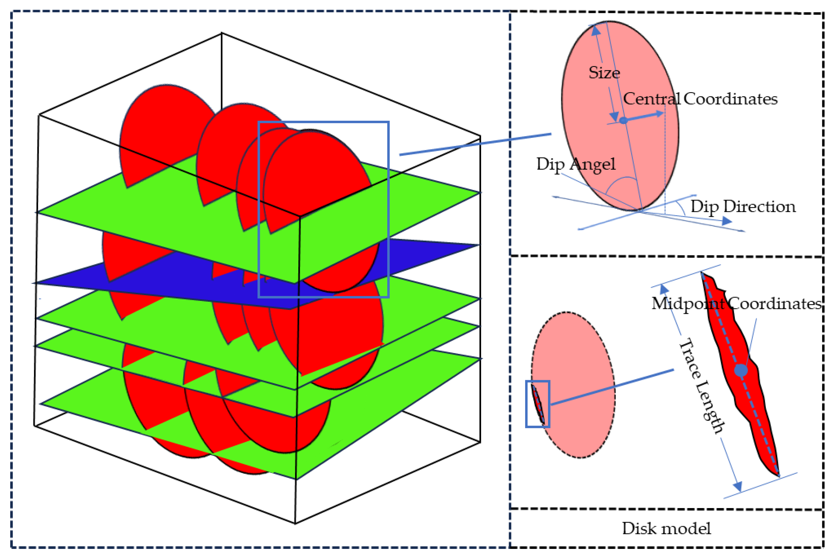
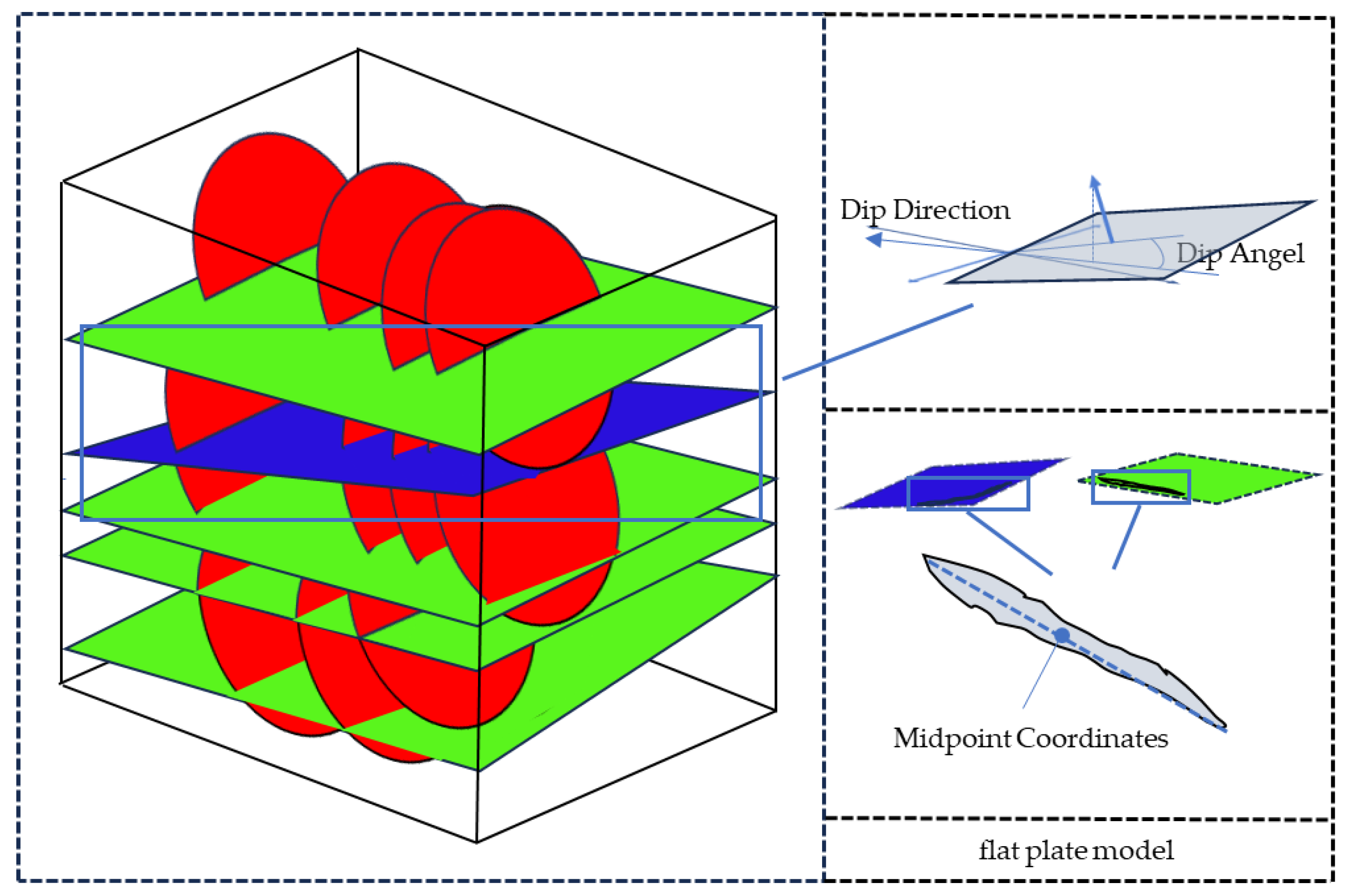
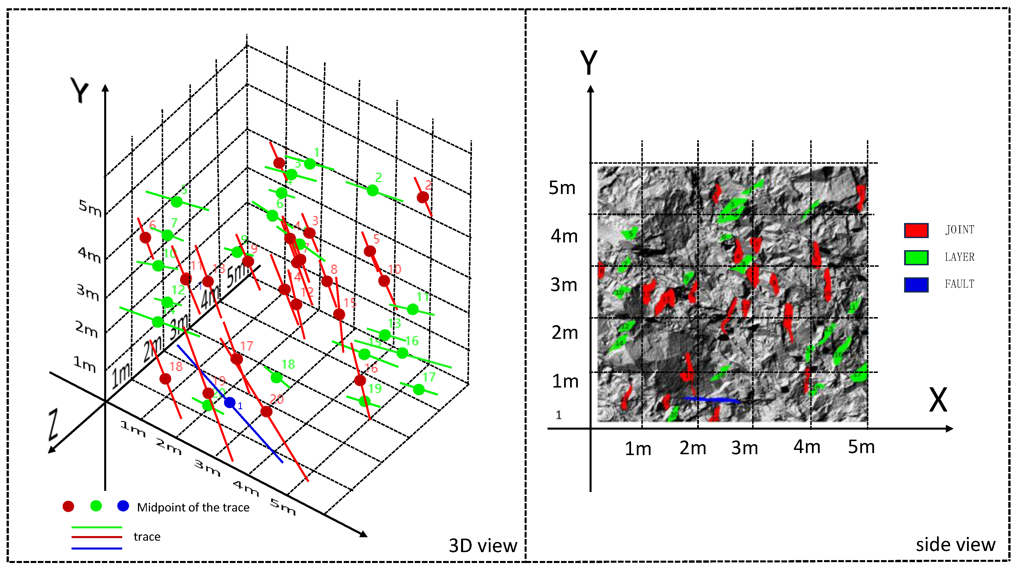
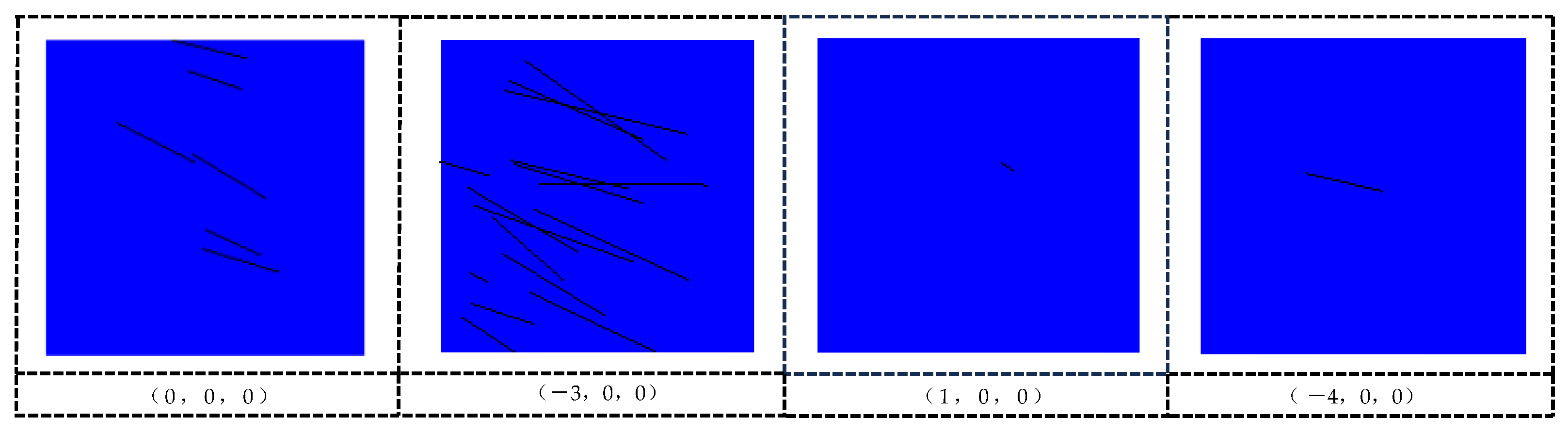
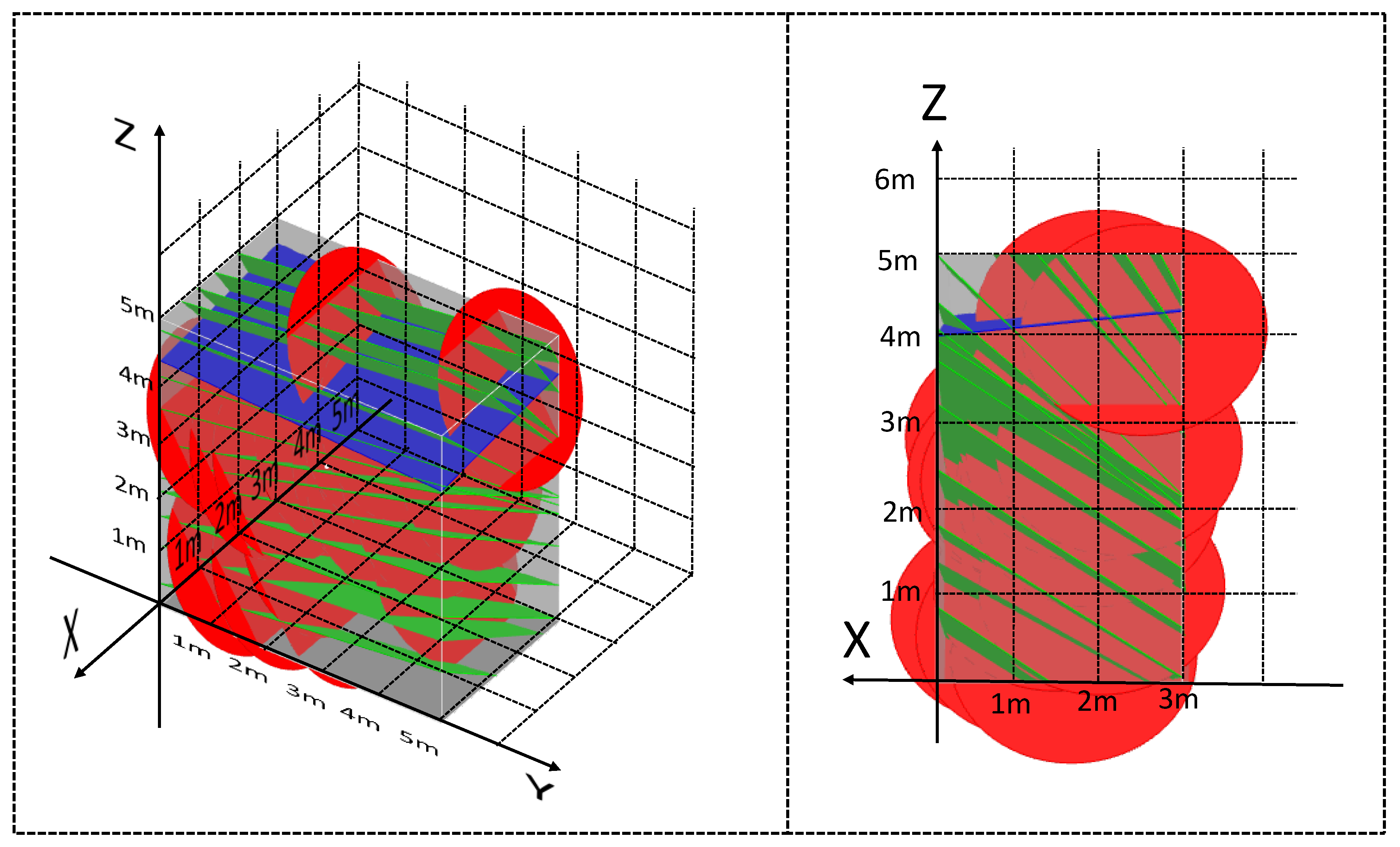
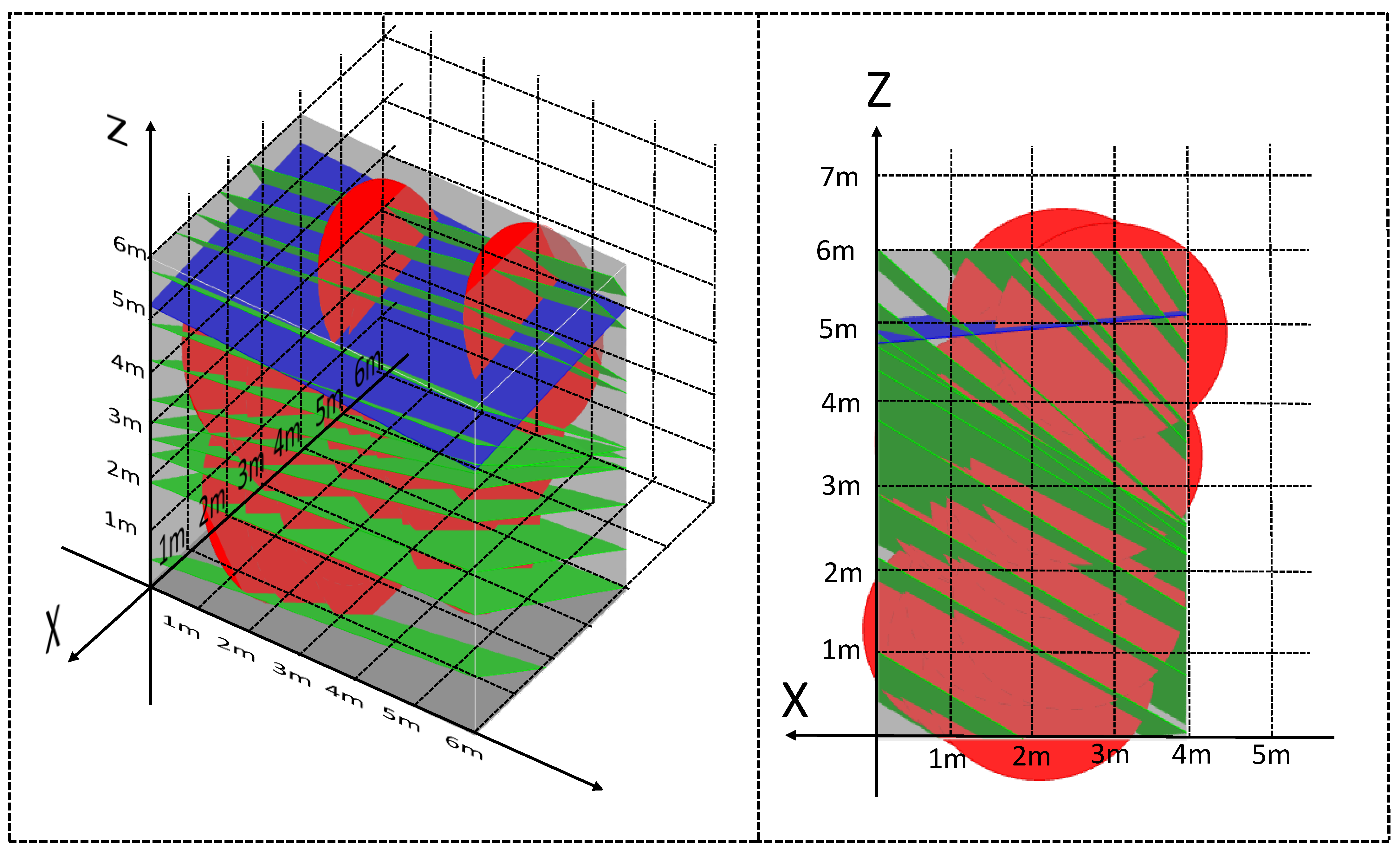
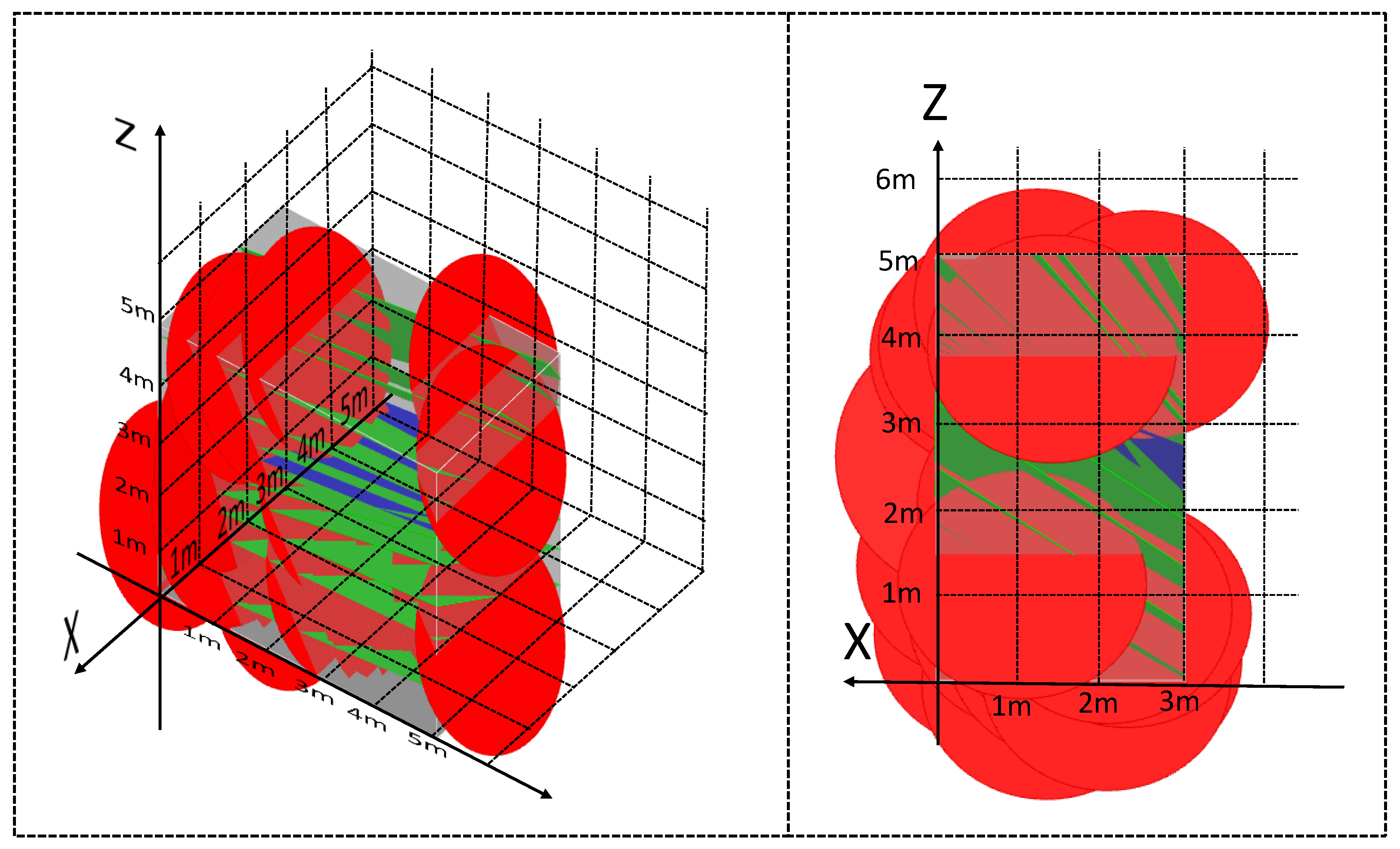
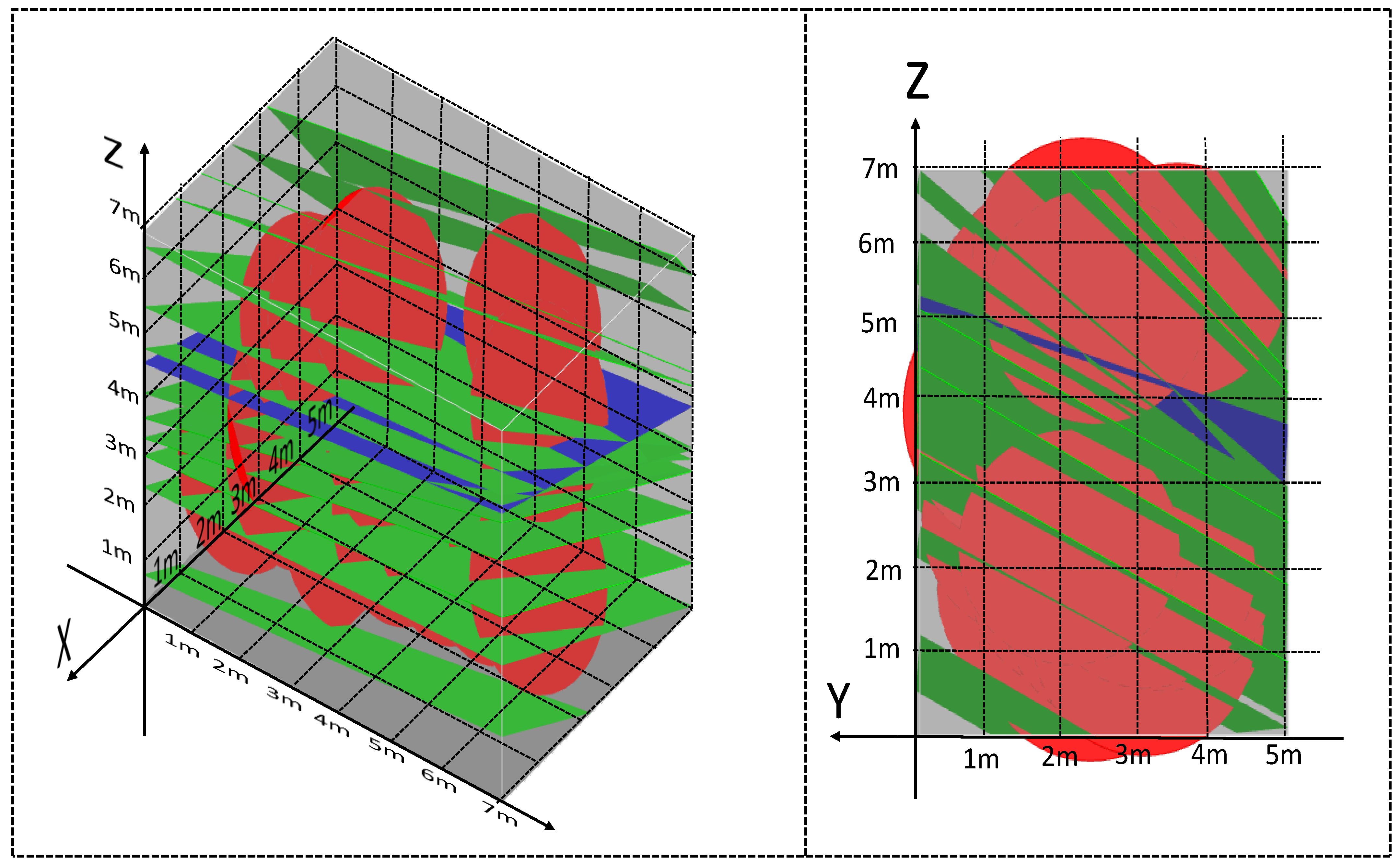
2.4. Structural 3D Modeling of Rock Mass

This section employs a deterministic method for modeling, characterizing joints, layers, and faults with different models. Joints are represented by disk models, which require parameters including the disk’s orientation, central coordinates, and persistence. The calculation of persistence and central coordinates follows: Previous studies have accurately described the relationships among spacing, surface density, volumetric density, and the persistence of structural planes. In the previous step, we extracted the spacing, while surface density and volumetric density can be directly calculated from the number of structural planes. Combining this information with prior research allows us to estimate the persistence of the structural planes. Based on this, geometric knowledge is utilized to deduce the relationship between persistence, trace length, orientation, and the central coordinates of the structural planes, thereby obtaining the 3D central coordinates of the structural planes.

Layer and fault models are characterized using the flat plate model, where the model parameters include the coordinates of a point on the model and its orientation. The coordinates of a point can be replaced by the trace center, thus eliminating the need for additional calculations.

For the rock mass model, it is necessary to continuously adjust its volume range to avoid edge effects.

After calculating the parameters of each model, the DFN model can be obtained by combining these models, as shown in Figure 2 below.

(1) Joint Disk Model:

Joint fractures typically do not penetrate through the entire rock mass region, so a disk model is chosen to represent them. The data required for the disk model in 3D space include the normal vector of the disk plane, the center coordinates of the disk, and the persistence of the disk. The normal vector can be calculated from the dip direction and dip angle of the plane. What needs to be calculated are the persistence and center coordinates. The 3D form of the joint model, along with the structural plane parameters it contains, is illustrated in Figure 3.

① Calculation of Disk Persistence:

As mentioned in previous research, the study object of this experiment is large planes with good influence; smaller, fragmented structural planes have been excluded. Since these structural planes are within a small-scale rock mass and their 3D distribution characteristics do not differ significantly, we decided to use the average persistence as the size of the disk model for the study.

In Ref. [26], the authors constructed 77 fracture network models with different lengths (D) and spacings (C) based on the rock mass fracture classification table from the International Society for Rock Mechanics (ISRM, 1978) (

Table 1. The Relationship Between Spacing, Persistence, and Volumetric Density.

	VCS1 0.04 m	VCS2 0.06 m	CS1 0.13 m	CS2 0.2 m	MS1 0.4 m	MS2 0.6 m	WS1 1.3 m	WS2 2 m	VWS 4 m
VHP 20 m	0.079	0.053	0.024	0.015	0.008	0.005	0.002	0.001	0.000
HP 15 m	0.141	0.094	0.043	0.028	0.014	0.009	0.004	0.002	0.001
MP1 10 m	0.318	0.212	0.097	0.063	0.031	0.021	0.009	0.006	0.003
MP2 6.5 m	0.753	0.502	0.231	0.150	0.075	0.050	0.023	0.015	0.007
LP1 3 m	3.536	2.357	1.088	0.707	0.353	0.235	0.108	0.070	0.035
LP2 2 m	7.957	5.305	2.448	1.591	0.795	0.530	0.244	0.159	0.079
VLP 1 m	31.831	21.220	9.794	6.366	3.183	2.122	0.979	0.636	0.318

). Refs. [27,28] proposed that when the structural surface representation model is a disk model, the persistence in Table 1 can be approximated as the model size. The relationship between persistence, spacing, and volumetric density is shown in Table 1.

In Table 1, VCS represents Very Close Spacing; M represents Moderate; W represents Wide; HP represents High Persistence; and L represents Light. The first row is the classification based on spacing, the first column is the classification based on structural plane size, and the middle section represents the corresponding bulk density.

The calculation formula for the trace line density ${\rho }_m^{\left(k\right)}$ is as follows:

$${\rho }_m^{\left(k\right)}={\displaystyle \frac{N^{\left(k\right)}}{W^2}}$$

(1)

$W$ represents the side length of the sampling window, $N^{\left(k\right)}$ represents the number of trace lines, and $k$ represents the number of groups of structural planes.

The expected value of the cosine of the acute angle γ between the normal vector of structural planes and the sampling window plane, approximated using directional samples, is given as follows:

$$E^{\left(k\right)}\left[cos\left(\gamma \right)\right]={\displaystyle \frac{\sum _{i=1}^{N^{\left(k\right)}}\sqrt{1-{sin}^2{\alpha }_i^{\left(k\right)}{sin}^2{\beta }_i^{\left(k\right)}}}{N^{\left(k\right)}}}$$

(2)

where $E^{\left(k\right)}\left[cos\left(\gamma \right)\right]$ denotes the expected value of $cos\left(\gamma \right)$ formed by the kth joint set. ${\alpha }_i^{\left(k\right)}$ and ${\beta }_i^{\left(k\right)}$ represent the dip direction and dip angle of the ith sample in the kth structural plane group, respectively.

By combining the trace line density ${\rho }_m^{\left(k\right)}$ with the expected value of the cosine of the acute angle γ, we can derive the formula for the volumetric density ${\rho }_V^{\left(k\right)}$:

$${\rho }_V^{\left(k\right)}={\displaystyle \frac{{\rho }_m^{\left(k\right)}}{E^{\left(k\right)}\left[cos\left(\gamma \right)\right]·\left[D^2/W+D\right]}}$$

(3)

From this, we can obtain the relationship between the fracture volumetric density and the fracture persistence [29,30]. By referring to Table 1, which relates volumetric density, spacing, and persistence, we can determine the average size of the disk model.

② Calculation of the disk center coordinates:

After obtaining the persistence and using the trace length and the midpoint of the trace obtained previously, we can calculate the center coordinates of the disk using the following formula:

$$\left\{\begin{array}{c}a=-\sqrt{\left[{(1/2)D}^2\right]-\left[{(1/2)l}^2\right]}cos{(\beta }_i-{\beta }_Q)\\ b=-\sqrt{\left[{(1/2)D}^2\right]-\left[{(1/2)l}^2\right]}sin({\beta }_i-{\beta }_Q)\\ c=\sqrt{\left[{(1/2)D}^2\right]-\left[{(1/2)l}^2\right]}cos{\alpha }_i\end{array}\right.$$

(4)

Among them, $(a,b,c)$ represents the direction from the center of the disk model to the center of the trace, ${\beta }_Q$ is the smaller quadrant angle when a structural surface is oriented such that it lies within the first quadrant and its ${\beta }_Q$ is 0 or 360, $D$ is the model size, and $l$ is the trace length. ${\alpha }_i,{\beta }_i$ represent the dip direction and dip angle, respectively.

Dividing the equation into quadrants:

For example, when ${\beta }_i\in \left(90,180\right)$:

$$\left\{\begin{array}{c}a=-\sqrt{\left[{(1/2)D}^2\right]-\left[{(1/2)l}^2\right]}cos{(\beta }_i-90)\\ b=-\sqrt{\left[{(1/2)D}^2\right]-\left[{(1/2)l}^2\right]}sin({\beta }_i-90)\\ c=\sqrt{\left[{(1/2)D}^2\right]-\left[{(1/2)l}^2\right]}cos{\alpha }_i\end{array}\right.$$

(5)

The relationship between the center coordinates of the disk and the center coordinates of the trace is:

$$\left\{\begin{array}{c}{x}_i=x_j-{\displaystyle \frac{a\sqrt{\left[{(1/2)D}^2\right]-\left[{(1/2)l}^2\right]}}{\sqrt{a^2+b^2+c^2}}}\\ y_i=y_j-{\displaystyle \frac{b\sqrt{\left[{(1/2)D}^2\right]-\left[{(1/2)l}^2\right]}}{\sqrt{a^2+b^2+c^2}}}\\ z_i=z_j-{\displaystyle \frac{c\sqrt{\left[{(1/2)D}^2\right]-\left[{(1/2)l}^2\right]}}{\sqrt{a^2+b^2+c^2}}}\end{array}\right.$$

(6)

$P_i=\left(x_i,y_i,z_i\right)$ is the center coordinates of the disk, and $P_j=\left(x_j,y_j,z_j\right)$ represents the center coordinates of the trace.

(2) Flat plate model for layers and faults:

Due to their extensive nature and the relatively small size of the experimental rock mass area, layers and faults are represented by a flat plate model that extends through the rock mass area. The data required for the flat plate model in 3D space include the normal vector of the plane and the starting point of the plane’s extension. The starting point of the plane’s extension is the midpoint of the trace line of the layer or fault structural surface, and the normal vector of the plane can be obtained from the dip direction and dip angle of the plane. The distribution of the layer and fault models in 3D space are shown in Figure 4.

(3) The Size of the Rock Mass Model

In order to avoid the occurrence of edge effects, it is necessary to expand the rock mass model until it includes all structural surfaces. The REV can be determined by setting up multiple observation windows to monitor the extension of structural planes within the rock mass.

(4) Surrounding Rock Classification

In the field of geotechnical engineering, blockiness serves as an efficient and effective indicator for evaluating rock mass quality and is widely used. In the 1998 Engineering Rock Mass Classification Standard, blockiness was correlated with rock mass quality grades, as shown in

Table 2. The relationship between the grade of rock mass quality and the degree of blockiness.

Classification of Blocking Degree	Rock Mass Grade	Percentage of Block
Non-blocky rock	V	0–10
Slightly blocky rock	IV	10–30
Moderately blocky rock	III	30–60
Blocky rock	I/II	More than 60

[31,32].

The influence of blocks with varying shapes and volumes on the calculation of blockiness was analyzed in detail in [33,34,35]. To account for these variations, weight factors were introduced for blocks of different volumes. The modified blockiness calculation method, incorporating these weighted parameters, is expressed as follows:

$$B_z=B_1+{\displaystyle \frac{1}{2}}{B}_2+{\displaystyle \frac{1}{3}}{B}_3+{\displaystyle \frac{1}{4}}{B}_4+{\displaystyle \frac{1}{5}}{B}_5$$

(7)

where $B_{1,2,3,4}$ variables represent the proportions of blocks with volumes in the ranges of 0~0.008, 0.008~0.030, 0.030~0.200, 0.200~1, and >1 m³, respectively, relative to the total volume of the rock mass. A specific table showing the correspondence between the two is presented in Table 2.

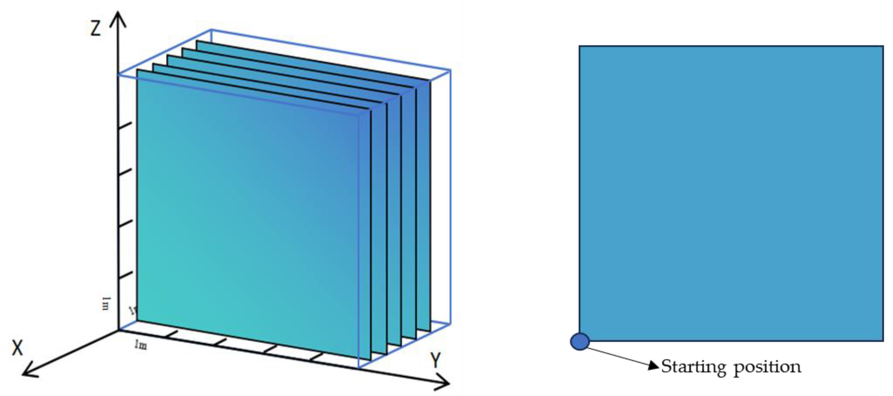
3. Example Verification

Dan Shan Station is located at the intersection of Heilongjiang Middle Road and Shimei’an Road. The strata mainly consist of a slightly weathered granite layer and moderately weathered tuff layer, with burial depths of approximately 23.2 m and 19.15 m, respectively. The rock mass grades are IV and V. The sampling area is primarily within the slightly weathered granite layer and the moderately weathered tuff layer. The following explanation will use pile number K16+790.5 as an example. First, based on the collected point cloud, a raster model of the rock mass area is constructed, as shown in Figure 5.

After obtaining the raster model, extract its slope, aspect, and elevation standard deviation. Perform ISODATA clustering on the slope, aspect, and elevation standard deviation, as shown in Figure 6. After clustering and zoning, filter the noisy clustering results using a window size greater than 20, as shown in Figure 7.

After removing smaller clusters through filtering, the DEV results for the remaining clustered zones were calculated, as presented in

Table 3. The calculation results of the DEV.

Cluster Partition	1	2	3	4	5	6	7	8
DEV	\	\	−0.0009	\	0.0001	−0.0017	−0.0038	−0.0004

. The degree of surface undulation of the structural plane calculated by $DEV$ can be normalized to represent the local surface roughness of the structural plane. $DEV\cong 0$ indicates that the central point and its neighborhood lie within the same plane.

The closer the DEV value is to 0, the more distinct the planar feature becomes. Therefore, values 3, 5, and 8 are identified as structural planes. Extract these values and further identify the more prominent and certain structural planes among them, as shown in Figure 8.

After obtaining the fracture surface grid model, the orientation can be quickly extracted using the arithmetic average method or the least squares method of the normal vectors. Based on this, the three-dimensional center coordinates of the fractures are obtained, and the spacing can then be calculated using geometric methods. For the trace lines, according to the needs of subsequent research, the fracture grids are converted into polygons and then into points in ARCGIS. By extracting the farthest endpoints of each trace line, its central coordinate and length can be calculated. Figure 9 shows the numbers of the structural surfaces, and

Table 4. The structural surface parameters of the Joint (Red).

Red	Dip Direction (°)		Dip Angle (°)	Space (m)	Red	Dip Direction (°)		Dip Angle (°)	Space (m)
1	90.47		59.69	/	11	92.16		50.47	0.754
2	89.55		63.62	0.035	12	96.88		58.54	0.380
3	87.92		57.87	0.004	13	100.86		59.01	0.334
4	95.80		54.56	1.152	14	103.55		68.60	0.066
5	91.33		57.09	0.278	15	89.60		66.55	0.580
6	92.39		50.63	1.042	16	93.29		58.57	0.488
7	90.55		53.66	0.028	17	91.77		52.41	0.200
8	83.70		63.06	0.156	18	92.88		54.89	0.161
9	105.99		66.68	0.156	19	96.35		54.97	1.309
10	90.95		60.39	0.049	20	87.65		54.30	0.122
Red	Midpoint Coordinates of Trace (m)			Trace Length (m)	Red	Midpoint Coordinates of Trace (m)			Trace Length (m)
1	2.52	4.51	−2.90	0.07	11	1.39	2.54	−2.03	0.13
2	4.77	4.34	−3.52	0.07	12	2.99	2.28	−2.70	0.14
3	3.16	3.55	−2.78	0.07	13	1.68	2.50	−2.20	0.14
4	2.88	3.40	−2.69	0.08	14	2.77	2.49	−2.67	0.16
5	4.10	3.40	−3.06	0.08	15	3.66	2.23	−2.84	0.15
6	0.66	3.03	−1.98	0.09	16	3.99	1.15	−2.98	0.18
7	3.04	3.07	−2.70	0.09	17	2.08	1.20	−2.37	0.19
8	3.48	2.79	−2.81	0.10	18	1.14	0.80	−1.82	0.19
9	2.21	2.88	−2.50	0.13	19	1.72	0.59	−2.14	0.25
10	4.28	2.87	−3.20	0.13	20	2.49	0.31	−2.59	0.30

and

Table 5. The structural surface parameters of Layers (Green) and Faults (Blue).

Green	Dip Direction (°)		Dip Angle (°)	Space (m)	Green	Dip Direction (°)		Dip Angle (°)	Space (m)
1	328.28		60.63	/	11	321.52		47.58	1.360
2	328.23		40.68	0.136	12	318.32		54.07	0.196
3	324.57		67.11	0.254	13	336.17		39.72	0.404
4	327.33		53.79	0.185	14	326.05		47.69	0.336
5	337.98		31.44	0.464	15	327.32		31.20	0.327
6	333.64		43.94	0.086	16	320.49		43.09	0.457
7	324.39		46.39	0.958	17	344.53		49.00	0.378
8	342.06		47.51	0.729	18	334.95		49.63	0.125
9	327.51		45.86	0.893	19	331.65		43.20	0.116
10	328.69		46.88	0.565	20	332.63		58.87	0.341
Blue	Dip Direction ($°$)		Dip Angle ($°$)	Space (m)	Blue	Dip Direction ($°$)		Dip Angle ($°$)	Space (m)
1	163.04		31.08	/	/	/		/	/
Green	Midpoint Coordinates of Trace (m)			Trace Length (m)	Green	Midpoint Coordinates of Trace (m)			Trace Length (m)
1	3.10	4.68	−2.90	0.08	11	4.69	2.43	−3.39	0.07
2	4.11	4.44	−3.13	0.12	12	1.10	2.07	−1.94	0.04
3	2.80	4.43	−2.83	0.08	13	4.30	1.94	−3.18	0.07
4	2.73	4.16	−2.67	0.05	14	0.97	1.72	−1.86	0.15
5	1.22	3.82	−2.02	0.12	15	4.00	1.57	−3.06	0.10
6	2.61	3.75	−2.60	0.07	16	4.59	1.70	−3.24	0.17
7	1.05	3.18	−2.01	0.06	17	4.87	1.13	−3.29	0.05
8	3.05	3.36	−2.69	0.12	18	2.61	0.89	−2.72	0.06
9	2.07	3.03	−2.43	0.05	19	4.05	0.80	−3.00	0.06
10	1.02	2.73	−1.83	0.09	20	1.76	0.41	−2.08	0.05
Blue	Midpoint Coordinates of Trace (m)			Trace Length (m)	Blue	Midpoint Coordinates of Trace (m)			Trace Length (m)
1	2.49	0.50	−1.06	0.23	/	/			/

display the structural surface parameters of the joints, layers and faults.

In the characterization of structural surfaces, due to differences in the model, it is necessary to distinguish between joints, layers, and faults. The sampling window persistence is 5 m × 5 m, resulting in a trace line density of 0.8. The inter-group spacing of the joint structural planes is 0.381 m, which is close to 0.4 m, so it is classified into the “MS1” category. Using formulas (1), (2), and (3), the calculated volumetric density is 20 structural planes divided by a volume of 75 m³, resulting in a value of 0.27. The cosine correction factor for the dip direction and angle is 0.5, leading to a structural plane model size of 3.5 m. However, Table 1 does not explicitly specify the exact relationship between spacing (0.4 m), volumetric density (0.27), and model size. Therefore, establishing an “MS1-LP1” model is considered the most appropriate choice. The average size of the disk model is 3 m. Thus, the center coordinates of the disk model can be obtained through calculations based on formulas 4, 5, and 6. For layers and faults, there is no need to perform such calculations. The subsequent analysis will use General Block to evaluate the degree of blockiness; the parameters of the three structural surface models are shown in

Table 6. Parameters of the Joint Model.

Joint	Center Coordinates (m)			Dip Direction (°)	Dip Angle (°)	Joint	Center Coordinates (m)			Dip Direction (°)	Dip Angle (°)
1	−4.47	5.00	5.40	90.47	59.69	11	−3.92	5.51	1.36	92.16	50.47
2	−4.22	5.43	4.79	89.55	63.62	12	−3.87	4.65	3.98	96.88	58.54
3	−4.20	5.47	3.74	87.92	57.87	13	−3.87	5.23	1.93	100.86	59.01
4	−4.16	5.27	5.76	95.80	54.56	14	−3.86	4.78	5.27	103.55	68.60
5	−4.15	4.51	3.93	91.33	57.09	15	−3.85	2.75	5.57	89.60	66.55
6	−4.06	5.02	6.12	92.39	50.63	16	−3.85	4.82	3.39	93.29	58.57
7	−4.02	5.33	2.66	90.55	53.66	17	−3.84	3.89	3.29	91.77	52.41
8	−4.01	4.33	4.46	83.70	63.06	18	−3.81	4.94	2.17	92.88	54.89
9	−3.93	4.22	2.21	105.99	66.68	19	−3.76	4.75	4.67	96.35	54.97
10	−3.93	4.96	5.03	90.95	60.39	20	−3.76	3.71	3.85	87.65	54.30

and

Table 7. Parameters of the Layer and Fault Models.

Layer	Starting Position (m)			Dip Direction (°)	Dip Angle (°)	Layer	Starting Position (m)			Dip Direction (°)	Dip Angle (°)
1	−3.75	4.63	3.05	328.28	60.63	11	−3.54	2.72	1.37	321.52	47.58
2	−3.73	3.39	4.61	328.23	40.68	12	−3.53	3.74	4.91	318.32	54.07
3	−3.69	4.64	1.81	324.57	67.11	13	−3.48	3.63	3.87	336.17	39.72
4	−3.67	4.37	3.22	327.33	53.79	14	−3.46	3.44	4.66	326.05	47.69
5	−3.65	3.22	3.34	337.98	31.44	15	−3.46	3.17	3.69	327.32	31.20
6	−3.65	3.27	4.13	333.64	43.94	16	−3.45	2.44	3.94	320.49	43.09
7	−3.64	3.11	4.46	324.39	46.39	17	−3.45	4.13	2.64	344.53	49.00
8	−3.63	4.69	1.03	342.06	47.51	18	−3.37	2.98	3.99	334.95	49.63
9	−3.62	3.00	3.55	327.51	45.86	19	−3.37	3.09	2.47	331.65	43.20
10	−3.57	3.25	3.82	328.69	46.88	20	−3.35	3.25	1.12	332.63	58.87
Fault	Starting position (m)			Dip Direction ($°$)	Dip Angle ($°$)	Fault	Starting position (m)			Dip Direction ($°$)	Dip Angle ($°$)
1	−2.46	1.66	2.96	163.04	31.08	/	/	/	/	/	/

.

In General Block, the rock mass model can only be built in the second quadrant. So, it is necessary to process the model parameters to ensure they conform to the coordinate system of the General Block. When using it, pay attention to adjusting the coordinate system, the parameters of the structural plane, and the relative position of the rock mass model.

Since the persistence of the sampling window is 5 m × 5 m, a 5 m × 5 m observation window is set every 0.5 m in the X direction starting from the origin, as shown in Figure 10 below. The layer and fault models penetrate the entire rock mass, so it is only necessary to observe the persistence of the joint model within the rock mass. The coordinate system in the figure is that of the software General Block. After selecting the starting point of the observation window, the window can be set along the direction perpendicular to the X-axis.

Due to the large number of observation window settings, only a portion of the observing results will be displayed. In the following text, it can be seen that the structural surfaces do not vanish at the points (0, 0, 0) and (−3, 0, 0). Therefore, it is necessary to expand the model in the X direction. When we continue to set up observation windows at (1, 0, 0) and (−4, 0, 0), it is found that the structural surfaces vanish, as shown in Figure 11.

Therefore, the X-direction dimension of the bedrock model is set to 5 m to ensure complete cutting. Through observation, it was found that the structural surfaces within the observation windows at the starting positions of (−1.5, 0, 0) and (−2, 0, 0) did not completely vanish in the Y direction. Thus, it is necessary to expand the observation windows to locate the vanishing positions. The original 5 m × 5 m windows were extended by 1 m to both the left and right. The distribution of structural surfaces within the observation windows after modifying the starting positions and window persistence is compared with the unmodified case, as shown in Figure 12.

By comparison, it can be seen that after expanding by 1 m in the Y direction, most of the structural surfaces vanished within the observation windows. Therefore, it is reasonable to expand the bedrock model by 1 m to both the left and right in the Y direction.

Similarly, observing the original observation windows reveals that the structural surfaces within the observation windows at (−2, 0, 0) and (−2.5, 0, 0) did not completely vanish in the Z direction. Therefore, the starting positions and window persistence of the observation windows at these two locations need to be adjusted in the Z direction.

Similarly, by comparison, it can be seen that after expanding by 1 m both upward and downward in the Z direction, most of the structural surfaces vanished within the observation windows. Therefore, it is reasonable to expand the bedrock model by 1 m both upward and downward in the Z direction, as shown in Figure 13.

By observing the extension of joints in the rock mass, the range of the rock mass can be preliminarily determined to be 5 m × 7 m × 7 m. Since not all observation results are presented, the next step is to establish a 3D model of the rock mass using GeoGebra3D to demonstrate the rationality of the selected range. The models before and after adjustment are shown in Figure 14 and Figure 15, respectively.

It can be seen from the model that the range of 5 m × 7 m × 7 m already includes almost all joint structural surfaces, avoiding edge effects.

We also conducted the same experiment on the rock masses at K16 + 792.4 and K16 + 795.7, as shown in Figure 16, Figure 17, Figure 18 and Figure 19, obtained the model parameters, and determined the model ranges as 6 m × 6 m × 4 m and 7 m × 7 m × 5 m, respectively.

After determining the scope of the REV, combining it with the structural plane model and importing it into General Block allows the blockiness calculation results to be obtained. The results are shown in

Table 8. The blockiness degree of the rock masses at K16+790.5, K16+792.4, and K16+799.5.

Number	Volume Proportion of Blocks at Five Different Scales (%)					Degree of Blockiness (%)
	B1	B2	B3	B4	B5
K16 + 790.5	73.30	14.40	12.23	0.03	0	12.25
K16 + 792.4	72.4	19.9	7.3	0.4	0	13.38
K16 + 795.7	66.7	21.4	10.6	1.3	0	8.86

below.

According to Table 2, the grades of the three rock masses are all Level IV and V, which matches the results of the geological exploration.

This demonstrates that the deterministic discrete fracture network (DFN) modeling approach, which characterizes different types of structural surfaces in a differentiated manner, indeed has a certain degree of reliability in reconstructing the true structure of small-scale rock masses.

4. Conclusions

(1) The discrete fracture network (DFN) model, established based on deterministically acquired structural surface parameters, can be effectively applied in practical engineering projects, offering greater efficiency and accuracy compared to traditional statistical methods and stochastic modeling theories.

(2) The hybrid model that represents joints as disks, layers, and faults as irregular planes can effectively simulate the real structural characteristics of rock masses, capturing the features of structural surfaces at different scales. This approach shows potential for future integration with the concept of Representative Elementary Volume (REV).

(3) The results show that the degree of blockiness and rock mass quality assessment derived from the rock mass structural models in the three experimental areas are consistent with the geological investigation data from the actual engineering site, thereby validating the reliability of the proposed modeling method.

References

1. Westaway, R.M.; Lane, S.N.; Hicks, D.M. The development of an automated correction -procedure for digital photogrammetry for the study of wide, shallow, gravel-bed rivers. Earth Surf. Process. Landf. 2000, 25, 209–226. [Google Scholar] [CrossRef]
2. Chandler, J. Effective application of automated digital photogrammetry for geomorphological research. Earth Surf. Process. Landf. 1999, 24, 51–63. [Google Scholar] [CrossRef]
3. Assali, P.; Grussenmeyer, P.; Villemin, T.; Pollet, N.; Viguier, F. Surveying and modeling of rock discontinuities by terrestrial laser scanning and photogrammetry: Semi-automatic approaches for linear outcrop inspection. J. Struct. Geol. 2014, 66, 102–114. [Google Scholar] [CrossRef]
4. Li, X.; Chen, J.; Zhu, H. A new method for automated discontinuity trace mapping on rock mass 3D surface model. Comput. Geosci. 2016, 89, 118–131. [Google Scholar] [CrossRef]
5. Umili, G.; Ferrero, A.; Einstein, H. A new method for automatic discontinuity traces sampling on rock mass 3D model. Comput. Geosci. 2013, 51, 182–192. [Google Scholar] [CrossRef]
6. Lane, S.N.; James, T.D.; Crowell, M.D. Application of Digital Photogrammetry to Complex Topography for Geomorphological Research. Photogramm. Rec. 2000, 16, 793–821. [Google Scholar] [CrossRef]
7. Long, J.C.S.; Remer, J.S.; Wilson, C.R.; Witherspoon, P.A. Porous media Equivalents for Networks of Discontinuous Fractures. Water Resour. Res. 1982, 18, 645–658. [Google Scholar] [CrossRef]
8. Cacciari, P.P.; Futai, M.M. Modeling a Shallow Rock Tunnel Using Terrestrial Laser Scanning and Discrete Fracture Networks. Rock Mech. Rock Eng. 2017, 50, 1217–1242. [Google Scholar] [CrossRef]
9. Hardebol, N.J.; Maier, C.; Nick, H.; Geiger, S.; Bertotti, G.; Boro, H. Multiscale fracture network characterization and impact on flow: A case study on the Latemar carbonate platform. J. Geophys. Res. Solid Earth 2015, 120, 8197–8222. [Google Scholar] [CrossRef]
10. Liu, R.; Jiang, Y.; Li, B.; Wang, X. A fractal model for characterizing fluid flow in fractured rock masses based on randomly distributed rock fracture networks. Comput. Geotech. 2015, 65, 45–55. [Google Scholar] [CrossRef]
11. Zhang, K.; Qi, F.; Bao, R.; Xie, J.B. Physical reconstruction and mechanical behavior of fractured rock masses. Bull. Eng. Geol. Environ. 2021, 80, 4441–4457. [Google Scholar] [CrossRef]
12. Guo, L.; Li, X.; Zhou, Y.; Zhang, Y.; Suo, P.; Tu, C. Three-dimensional network simulation of structural planes in fractured rock masses based on the coupling of stochastic and deterministic methods. Rock Soil Mech. 2016, 37, 2636–2644, 2653. [Google Scholar]
13. Wang, S.H.; Mu, X.J.; Zhang, H.; Zhang, S.C. Spatial Modeling of Refined Structural Plane of Rock Mass and Block Stability Analysis. J. Northeast Univ. (Nat. Sci.) 2012, 8, 1186–1189. [Google Scholar]
14. Bandyopadhyay, K.; Mallik, J. An optimum solution for coal permeability estimation from mesoscopic scale calibrated stochastic and deterministic discrete fracture network models. Fuel 2022, 331, 125626. [Google Scholar] [CrossRef]
15. Pan, D.; Li, S.; Xu, Z.; Zhang, Y.; Lin, P.; Li, H. A deterministic-stochastic identification and modelling method of discrete fracture networks using laser scanning: Development and case study. Eng. Geol. 2019, 262, 105310. [Google Scholar] [CrossRef]
16. Liu, T.; Deng, J. Photogrammetry-Based 3D Textured Point Cloud Models Building and Rock Structure Estimation. Appl. Sci. 2023, 13, 4977. [Google Scholar] [CrossRef]
17. Jiang, S.H.; Chen, J.D.; Zou, Z.Y. Stability analysis of jointed rock slopes based on a universal elliptical disc model and its realization in 3DEC. Chin. J. Rock Mech. Eng. 2023, 42, 1610–1622. [Google Scholar]
18. Hekmatnejad, A.; Emery, X.; Vallejos, J.A. Robust estimation of the fracture diameter distribution from the true trace length distribution in the Poisson-disc discrete fracture network model. Comput. Geotech. 2018, 95, 137–146. [Google Scholar] [CrossRef]
19. Zhao, X.Y.; You, Y.C.; Hu, X.Y.; Li, J.; Li, Y. Classified-staged-grouped 3D modeling of multi-scale fractures constrained by genetic mechanisms and main controlling factors: A case study on biohermal carbonate reservoir of the Upper Permian Changxing Fm. in Yuanba area, Sichuan Basin. Oil Gas Geol. 2023, 44, 213–225. [Google Scholar]
20. Zhan, D.; Shao, Z.P.; Zeng, L.; Wang, Y.J.; Tong, L. A Study on Fracture Modelling of the Bedrock Reservoir in Dongping Gas Field, Qaidam Basin. J. Southwest Pet. Univ. (Sci. Technol. Ed.) 2019, 41, 71–79. [Google Scholar]
21. Zhou, Q.M.; Liu, X.J. Analysis of errors of derived slope and aspect related to DEM data properties. Comput. Geosci. 2004, 30, 369–378. [Google Scholar] [CrossRef]
22. Zhang, P.; Li, J.; Yang, X.; Zhu, H. Semi-automatic extraction of rock discontinuities from point clouds using the ISODATA clustering algorithm and deviation from mean elevation. Int. J. Rock Mech. Min. Sci. Géoméch. Abstr. 2018, 110, 76–87. [Google Scholar] [CrossRef]
23. Zhang, P.; Qian, X.; Guo, X.; Yang, X.; Li, G. Automated demarcation of the homogeneous domains of trace distribution within a rock mass based on GLCM and ISODATA. Int. J. Rock Mech. Min. Sci. Géoméch. Abstr. 2020, 128, 104249. [Google Scholar] [CrossRef]
24. Wang, X.M.; Niu, R.Q.; Wu, T. Research on lithology intelligent classification for Three Gorges Reservoir area. Rock Soil Mech. 2010, 31, 2946–2950. [Google Scholar]
25. Guo, J.T.; Zhang, Z.R.; Mao, Y.C.; Liu, S.J. Automatic Discontinuity Classification and Parameter Calculation from Rock Mass 3D Point Cloud. Dong Bei Da Xue Xue Bao/J. Northeast. Univ. 2020, 41, 1161–1166. [Google Scholar]
26. Xia, L.; Zheng, Y.; Yu, Q. Estimation of the REV size for blockiness of fractured rock masses. Comput. Geotech. 2016, 76, 83–92. [Google Scholar] [CrossRef]
27. Xia, L.; Xie, J.; Yu, Q.C. Influence of statistical distribution dispersion in the fracture size on blockiness REV of fractured rock masses. Hydrogeol. Eng. Geol. 2019, 46, 112–118. [Google Scholar]
28. Zhang, L.L.; Zhang, X.; Wang, Y. Determining of the REV for fracture rock mass of very low ductility. Hydrogeol. Eng. Geol. 2011, 38, 20–25. [Google Scholar]
29. Zhang, Q.; Wang, X.; Zhu, H.; Zhang, K.; Li, X. Mixture distribution model for three-dimensional geometric attributes of multiple discontinuity sets based on trace data of rock mass. Eng. Geol. 2022, 311, 106915. [Google Scholar] [CrossRef]
30. Zhang, Q.; Wang, X.; He, L.; Tian, L. Estimation of Fracture Orientation Distributions from a Sampling Window Based on Geometric Probabilistic Method. Rock Mech. Rock Eng. 2021, 54, 3051–3075. [Google Scholar] [CrossRef]
31. Chen, Q.F.; Wei, C.S.; Niu, W.J.; Chen, D.Y.; Feng, C.H.; Fan, Q.Y. Stability classification of roadway roof in fractured rock mass based on blockiness theory. Rock Soil Mech. 2014, 35, 2901–2908. [Google Scholar]
32. He, D.Z.; Hu, B.; Yao, W.M.; Li, L.C.; Li, H.Z. Stability grading method for open-pit slope based on blockiness and cloud model. Min. Metall. Eng. 2017, 37, 6–10. [Google Scholar]
33. Chen, Q.F.; Niu, W.J.; Zheng, W.S.; Liu, J.G.; Yin, T.C.; Fan, Q.Y. Correction of the problems of blockiness evaluation method for fractured rock mass. Rock Soil Mech. 2018, 39, 3727–3734. [Google Scholar]
34. The Ministry of Water Resources of the People’s Republic of China. GB50218-94 Standard for Engineering Classification of Rock Masses; China Planning Press: Beijing, China, 1994.
35. Ding, Z.J.; Zheng, J.; Lü, Q.; Deng, J.H.; Tong, M.S. Discussion on calculation methods of quality index of slope engineering rock mass in Standard for engineering classification of rock mass. Rock Soil Mech. 2019, 40, 275–280. [Google Scholar]
Figure 1. Flow Chart of Deterministic Discrete Fracture Network Model.
Applsci 15 06264 g001
Figure 2. Estimation of the 3D Distribution Morphology of Integral Structural Surfaces.
Applsci 15 06264 g002
Figure 3. The distribution of the 3D joint model.
Applsci 15 06264 g003
Figure 4. The distribution of the Layer and Fault 3D Models.
Applsci 15 06264 g004
Figure 5. Rock Surface Raster Model.
Applsci 15 06264 g005
Figure 6. (a) Slope, (b) Aspect, (c) Elevation standard deviation, and (d) ISODATA clustering results.
Applsci 15 06264 g006
Figure 7. Comparison before and after filtering.
Applsci 15 06264 g007
Figure 8. Extraction of Structural Surfaces.
Applsci 15 06264 g008
Figure 9. The number of the structural surface at K16+790.5.
Applsci 15 06264 g009
Figure 10. Set up observation windows.
Applsci 15 06264 g010
Figure 11. The observation windows at (1, 0, 0) and (−4, 0, 0).
Applsci 15 06264 g011
Figure 12. The observation windows at (−2, −1, 0) and (−1.5, −1, 0).
Applsci 15 06264 g012
Figure 13. The observation windows at (−2, 0, −1) and (−2.5, 0, −1).
Applsci 15 06264 g013
Figure 14. GeoGebra3D model before adjustment in K16+790.5.
Applsci 15 06264 g014
Figure 15. GeoGebra3D model after adjustment in K16+790.5.
Applsci 15 06264 g015
Figure 16. GeoGebra3D model before adjustment in K16+792.4.
Applsci 15 06264 g016
Figure 17. GeoGebra3D model after adjustment in K16+792.4.
Applsci 15 06264 g017
Figure 18. GeoGebra3D model before adjustment in K16+795.7.
Applsci 15 06264 g018
Figure 19. GeoGebra3D model after adjustment in K16+795.7.
Applsci 15 06264 g019