A Transformer-Based Reinforcement Learning Framework for Sequential Strategy Optimization in Sparse Data

Abstract

A deep reinforcement learning framework is presented for strategy generation and profit forecasting based on large-scale economic behavior data. By integrating perturbation-based augmentation, backward return estimation, and policy-stabilization mechanisms, the framework facilitates robust modeling and optimization of complex, dynamic behavior sequences. Experimental evaluations on four distinct behavior data subsets indicate that the proposed method achieved consistent performance improvements over representative baseline models across key metrics, including total profit gain, average reward, policy stability, and profit–price correlation. On the sales feedback dataset, the framework achieved a total profit gain of 0.37, an average reward of 4.85, a low-action standard deviation of 0.37, and a correlation score of $R^2=0.91$. In the overall benchmark comparison, the model attained a precision of 0.92 and a recall of 0.89, reflecting reliable strategy response and predictive consistency. These results suggest that the proposed method is capable of effectively handling decision-making scenarios involving sparse feedback, heterogeneous behavior, and temporal volatility, with demonstrable generalization potential and practical relevance.

1. Introduction

Driven by the wave of digitalization, massive volumes of economic behavior data have become a critical foundation for modern enterprises to support decision-making and optimization processes [1]. These data primarily encompass transaction records, click behavior, browsing paths, and price responses, capturing user decision-making patterns and market dynamics across various economic activities [2]. With the continuous advancement of big data technologies and computational capabilities, these large-scale datasets offer unprecedented opportunities for enterprises to refine pricing strategies and forecast revenues with higher accuracy [3,4]. Nevertheless, extracting meaningful insights from complex, high-dimensional, and delayed-feedback economic behavior data remains a significant challenge in the field of intelligent pricing [5]. Traditional pricing strategies often rely on static statistical models or manually defined rules, which tend to be inadequate in handling dynamic market environments [6]. Such approaches demonstrate limited flexibility and effectiveness, particularly in scenarios involving diverse product types, intricate user behavior, and intense market competition [7,8]. Specifically, static pricing models are unable to dynamically adjust prices, making them unsuitable for rapidly changing markets. Rule-based methods, on the other hand, depend heavily on expert experience and often fail to quantitatively model complex economic behavior and market feedback [9]. Moreover, economic behavior data are characterized by high dimensionality, heterogeneity, temporal dependence, and sparsity, which makes it difficult for traditional models to generalize effectively or cope with the data’s inherent complexity [10]. Although static pricing approaches were among the earliest methods applied in market settings, they generally set prices based on historical data and market patterns [11]. While effective in simple markets with a single product and stable conditions, such methods exhibit substantial limitations in complex real-world scenarios [12], such as the inability to promptly update prices or account for consumer heterogeneity and intricate market behavior [13]. Regression-based dynamic pricing methods typically involve building regression models to estimate the relationship between price and sales volume, followed by pricing adjustments based on market feedback [14]. While these methods can partially address demand fluctuations, their limitations are evident. First, regression models often assume a fixed relationship between demand and price; however, in complex market environments, this relationship is highly nonlinear and dynamic, which cannot be adequately captured by standard regression techniques [15]. Second, these models usually presume immediate and continuous feedback from the market, whereas, in reality, feedback is frequently delayed and sparse, leading to uncertainty that regression models are ill-equipped to manage [16,17].

With the advancement of deep learning technologies, data-driven pricing strategies have attracted increasing attention in both academic and industrial domains. Deep learning enables multi-layer neural networks to extract abstract representations from complex economic behavior data, thereby facilitating more accurate and flexible decision-making processes [18,19]. In particular, deep reinforcement learning (DRL), which combines the perceptual capabilities of deep networks with the sequential decision-making mechanisms of reinforcement learning, has emerged as a highly promising paradigm [20]. Among the various DRL methods, the deep Q-network (DQN) represents a fundamental breakthrough. By leveraging deep neural networks to approximate the Q-value function, DQN effectively addresses the scalability issues encountered by traditional Q-learning in high-dimensional state spaces [21,22]. Through end-to-end interactions with the environment, DQN enables direct learning of pricing strategies from feedback signals [23]. Compared with conventional approaches, DQN exhibits superior generalization performance and adaptability to dynamic market environments. For example, Liang et al. constructed a Dueling DQN-based presale pricing model capable of adapting to complex dynamics in multi-phase sales processes, which demonstrated strong policy generalization across various product categories, thereby improving retail profitability [24]. Zhu et al. developed a reinforcement learning framework for multi-flight pricing, validating the policy convergence and generalization performance of DQN and other algorithms under high-dimensional state spaces and competitive market conditions such as high-speed rail interference [25]. Narayan et al. further demonstrated the profit advantages of DQN in high-volatility pricing scenarios within intelligent transportation systems [26]. Recent studies have also extended DRL to incorporate more diverse behavioral signals, such as inventory levels, competitor pricing, and user browsing behavior [27]. Effectively integrating these multidimensional features remains a core challenge in pricing-strategy modeling. To address this issue, Avramelou et al. proposed a multimodal financial embedding approach to fuse price and sentiment data while enabling interpretable weighting of each modality’s influence on the decision outcomes [28]. Yan et al. designed a multi-source information fusion framework that integrates graph convolutional networks and large language models for sector rotation-based asset allocation, demonstrating strong performance under multi-source financial data scenarios [29]. Wang et al. developed a high-dimensional state representation framework capable of capturing cross-feature interactions and enhancing the robustness of pricing decisions [30]. In addition, hybrid models have also been explored. Chen et al. introduced a K-means–LSTM hybrid model based on dynamic time warping (DTW) clustering to predict financial time series [31]. Liu et al. developed a DDPG-based pricing strategy for electric vehicle aggregators under evolving market conditions [32]. Moreover, Yin et al. integrated DRL with game-theoretic reasoning to derive optimal pricing strategies under strategic competition using Nash equilibrium solutions [6]. He et al. proposed a hybrid DRL model based on a bi-level Markov decision process that integrates day-ahead and real-time pricing mechanisms for coordinated modeling of supply–demand dynamics in electricity markets [33]. These recent developments underscore the increasing structural sophistication of DRL-based pricing frameworks and highlight the importance of designing architectures capable of learning from heterogeneous, delayed, and interactive economic feedback signals.

A novel framework for pricing-strategy generation and revenue prediction based on DRL is proposed in this work. By introducing a deep Q-network architecture and incorporating high-dimensional state modeling, price perturbation enhancement, and delayed-reward reevaluation mechanisms, the framework enables dynamic responses to user behavior and progressive optimization of pricing strategies. The key contributions of this work are summarized as follows:

• High-dimensional heterogeneous state modeling and long short-term return balancing: A DRL-based pricing framework is proposed that effectively addresses the challenges of modeling high-dimensional heterogeneous states and balancing short- and long-term returns using large-scale economic behavior data.
• Reward enhancement via price perturbation and delayed-feedback revisitation: A novel reward enhancement mechanism is designed based on price perturbation and delayed-feedback tracing, significantly improving model stability and applicability in real-world big data environments, especially under delayed-feedback and sparse-data conditions.
• Comprehensive empirical validation and multi-scenario applicability: Extensive experiments on multiple real-world economic datasets demonstrate the proposed method’s superior performance in terms of revenue growth rate, pricing stability, and policy generalization compared to existing baseline approaches.

A subset of the data samples and the full source code will be made publicly available at 28 May 2025 https://github.com/user837498178/DRL after acceptance.

2. Related Works

2.1. Traditional Pricing Models and Strategies

Traditional pricing models have been extensively applied across various economic domains, particularly in product pricing and market strategy optimization [34]. Classical pricing approaches primarily include static pricing methods, regression-based dynamic pricing models, and pricing game strategies derived from game theory [35]. While each of these methods demonstrates value under specific market conditions, limitations are evident when addressing high-dimensional state modeling and real-time feedback [36]. Static pricing methods represent one of the earliest and most widely adopted pricing strategies. The core idea involves predefining prices based on historical data and market patterns, without accommodating dynamic market changes [37]. Such methods are typically suitable for relatively stable markets with predictable demand [38]. However, in volatile markets influenced by complex consumer behavior and competitive pricing, static pricing approaches often lack efficiency and adaptability [39]. Consequently, these models generally rely on averages or heuristic rules derived from historical data but lack the capacity for dynamic adjustments. To address these shortcomings, regression-based dynamic pricing models have been introduced [40]. These models dynamically adjust prices by establishing functional relationships between price, sales, and demand. Regression analysis is commonly used to model the dependency between pricing and demand. A representative linear regression model is expressed as

$$y={\beta }_0+{\beta }_1{x}_1+{\beta }_2{x}_2+\dots +{\beta }_n{x}_n+ϵ,$$

(1)

where y denotes sales or demand, $x_1,x_2,\dots ,x_n$ represent feature variables related to price and market conditions, ${\beta }_0,{\beta }_1,\dots ,{\beta }_n$ are regression coefficients, and $ϵ$ is the error term. This approach assumes a linear or otherwise regressive relationship between price and demand. However, in practical scenarios, the relationship between pricing and consumer demand is often nonlinear and influenced by various factors, such as psychological behavior and seasonal market fluctuations. Therefore, regression-based dynamic pricing methods tend to lack accuracy and stability when faced with such complexity. Pricing game strategies derived from game theory have been widely applied in competitive market scenarios, especially under multi-agent competition [41]. Game theory offers a systematic framework for analyzing strategic behavior among market participants, where pricing is often a critical decision variable [42]. Typical game-theoretic models involve defining the players, strategy spaces, and payoff functions, from which equilibrium pricing can be derived [43]. For example, in a classical Nash equilibrium model, each participant chooses the optimal strategy considering the strategies of others. The payoff function can be expressed as

$$u_i(p_1,p_2,\dots ,p_n)=\mathrm{profit}\mathrm{function}(p_i,p_1,p_2,\dots ,p_n),$$

(2)

where $u_i$ denotes the profit of the i-th participant, $p_1,p_2,\dots ,p_n$ are the pricing strategies of all participants, and the profit function reflects how revenue varies under different pricing scenarios. Although game-theoretic approaches provide a theoretical framework for analyzing pricing competition, practical application is constrained by the dynamic nature of markets, nonlinear price feedback, and the unpredictability of competitor behavior. These models often assume fully rational agents, thereby overlooking the complexity of consumer behavior and the presence of irrational market factors, which limits their applicability in complex real-world environments [44].

2.2. Applications of Deep Reinforcement Learning in Pricing Scenarios

DRL, which integrates reinforcement learning (RL) with deep learning, has gained substantial traction in various practical domains in recent years [45,46]. RL, as a major branch of machine learning, enables agents to learn optimal strategies by interacting with the environment. The fundamental components of RL include the agent, environment, state, action, and reward [47]. An agent selects an action under a given state and updates its strategy based on feedback (reward or penalty) from the environment, aiming to maximize the cumulative reward. The value function in RL is defined as

$$V\left(s\right)=\mathbb{E}[\sum _{t=0}^{\infty }{\gamma }^t{r}_t|s_0=s],$$

(3)

where $V\left(s\right)$ represents the expected value under state s, $r_t$ is the reward at time t, and $\gamma$ is the discount factor representing the attenuation of future rewards. By iteratively updating strategies, agents can discover optimal policies in complex environments. In DRL, deep neural networks are employed to approximate value or policy functions, effectively addressing the computational challenges posed by high-dimensional state spaces faced by traditional RL [48]. Among the most representative DRL algorithms is the deep Q-network (DQN), which combines Q-learning with deep learning to approximate the Q-function using neural networks, enabling the model to handle complex and high-dimensional state spaces [49]. The Q-function is defined as

$$Q(s,a)=\mathbb{E}[r_t+\gamma \underset{a^{\prime }}{max}Q(s^{\prime },a^{\prime })|s_t=s,a_t=a],$$

(4)

where $Q(s,a)$ denotes the expected return from taking action a in state s, $s^{\prime }$ is the next state, $r_t$ is the immediate reward, $\gamma$ is the discount factor, and ${max}_{a^{\prime }}Q(s^{\prime },a^{\prime })$ represents the maximum Q-value for all possible actions in state $s^{\prime }$. Through end-to-end neural network training, DQN can learn optimal pricing policies in complex environments [50]. Additionally, algorithms such as deep deterministic policy gradient (DDPG) and asynchronous advantage actor–critic (A3C) have also been applied in pricing decisions, particularly in scenarios involving continuous action spaces and high-dimensional state representations [51]. DDPG is a policy-gradient-based algorithm that estimates both the policy and value functions through deep networks to solve continuous control problems [52]. A3C leverages asynchronous multi-threaded training to enhance efficiency and has demonstrated strong performance in various tasks [53]. Despite the promising performance of DRL in pricing applications, several challenges remain. First, training DRL models typically requires a large volume of interaction data, which may be difficult to obtain in real-world pricing scenarios [54]. Second, due to the dynamic and complex nature of economic environments, DRL models are prone to overfitting and training instability [55]. Furthermore, delayed rewards and partial feedback complicate the learning process, making the design of effective reward functions and the mitigation of these issues a critical area for future research.

2.3. Revenue Prediction and Economic Behavior Modeling

Revenue prediction constitutes a core problem in economics, particularly in sales forecasting and market analysis, where accurate prediction supports the development of optimized pricing strategies [56]. In recent years, deep learning methods—especially those tailored to sequential data such as long short-term memory (LSTM) networks and transformers—have been widely adopted for sales forecasting [57]. LSTM networks, designed for sequence modeling, introduce gated mechanisms that effectively address the vanishing gradient problem observed in traditional recurrent neural networks (RNNs). The fundamental components of an LSTM unit include the input, forget, and output gates, with the update equations as follows:

$$f_t=\sigma (W_f·[h_{t-1},x_t]+b_f)$$

(5)

$$i_t=\sigma (W_i·[h_{t-1},x_t]+b_i)$$

(6)

$$\widetilde{C_t}=tanh(W_C·[h_{t-1},x_t]+b_C)$$

(7)

$$C_t=f_t\ast C_{t-1}+i_t\ast \widetilde{C_t}$$

(8)

$$o_t=\sigma (W_o·[h_{t-1},x_t]+b_o)$$

(9)

$$h_t=o_t\ast tanh\left(C_t\right),$$

(10)

where $f_t$ is the output of the forget gate, $i_t$ is the input gate, $\widetilde{C_t}$ is the candidate cell state, $C_t$ is the updated cell state, $o_t$ is the output gate, and $h_t$ is the hidden state. The LSTM structure enables the modeling of long-range dependencies, which play a vital role in revenue forecasting. Transformer models, built on self-attention mechanisms, offer advantages over LSTM in handling long sequences through parallel processing [58]. The core operation of the self-attention mechanism is formulated as

$$\mathrm{Attention}(Q,K,V)=\mathrm{softmax}\left({\displaystyle \frac{Q{K}^T}{\sqrt{d_k}}}\right)V,$$

(11)

where Q, K, and V represent the query, key, and value matrices, respectively, and $d_k$ denotes the dimensionality of the keys. This mechanism enables the modeling of dependencies between all positions in a sequence, facilitating more expressive representations. Although LSTM and transformer models have demonstrated strong performance in revenue forecasting, several challenges persist. First, the complexity and variability of temporal data make models susceptible to noise interference [59]. Second, these models often assume a fixed sequential relationship in data; however, in practice, user behavior is influenced by seasonal effects, promotional campaigns, and other external factors. Addressing the non-stationarity of time-series data remains a key direction for future research [60].

3. Materials and Method

3.1. Dataset Collection

The dataset utilized in this study was collected from major e-commerce platforms across multiple representative industries over a continuous period from January 2023 to December 2023. The data exhibit a well-defined time-series structure and encompasses diverse behavioral features. To ensure both the practical relevance and generalizability of the experimental results, four core types of economic behavior data were gathered: product pricing records, sales feedback, user browsing behavior, and inventory levels. Data sources included leading platforms such as JD (jd.com), Taobao (taobao.com), Suning (suning.com), and Vipshop (vip.com). For each category, between 200,000 and 400,000 complete records were collected, resulting in a total dataset size exceeding 1,000,000 entries. The data were collected at a daily granularity, enabling robust time-series modeling, as shown in

Table 1. Behavior data subtype statistics.

Data Type	Source Platforms	Number of Records	Collection Period
Product Pricing Records	JD, Taobao, Suning	205,890	April–December 2023
Sales Feedback	Taobao, Suning, Vipshop	280,312	July–December 2023
User Browsing Behavior	Taobao, Suning	279,034	January–June 2023
Inventory Levels	JD, Taobao	348,910	February–October 2023
Total	——	1,000,000+	Daily Time Series

.

During the data collection process, an automated scraping system was developed using Python 3.13-based tools, including Scrapy and Selenium. While these tools enabled the acquisition of large-scale behavior data from multiple e-commerce platforms, their use also introduced potential risks, such as parsing errors caused by frequent website structure changes, anti-scraping mechanisms, and inconsistent page templates. To mitigate these issues, several safeguards were employed: structural schema validation was applied during crawling to ensure field consistency, periodic manual sampling was conducted to audit data quality, and records with missing or anomalous key attributes were filtered out during preprocessing. Additionally, data collection was performed within a constrained time window to minimize discrepancies due to platform-side updates. For the pricing records, data were periodically retrieved from product detail pages and promotional listings, capturing listed prices, discount prices, and associated timestamps. The pricing fields followed a consistent structure, incorporating price fluctuation ranges, update frequency, and promotional tags, which effectively reflected the dynamic characteristics of pricing strategies. Sales feedback data were obtained from historical transaction statistics and monthly sales rankings, with fields including daily sales volume, cumulative monthly sales, and sales ranks, normalized using timestamp alignment for consistent analysis. Browsing behavior data were extracted from page popularity indicators, click-tracking modules, and redirection logs in recommendation zones. The collected fields included click frequency, navigation depth, and average session duration, providing insight into user engagement patterns. Inventory data were inferred from stock status prompts, restock frequency indicators, and seller dispatch cycles on product pages, and further refined through integration with pricing and sales information to approximate real-world supply–demand dynamics.

3.2. Data Preprocessing and Augmentation

In the framework of DRL, data preprocessing and augmentation constitute critical steps to ensure model stability and accuracy in complex market environments. In practical applications, economic behavior data often suffer from missing values and outliers. Furthermore, due to delayed market feedback, handling lagged data and enhancing data diversity have emerged as core challenges in preprocessing. To address these issues, several effective preprocessing and augmentation techniques have been proposed to improve learning efficiency and model robustness. Initially, the imputation of missing values and treatment of outliers are essential preprocessing procedures. In economic behavior datasets—particularly transaction logs and market feedback—missing or anomalous data are frequently encountered. Missing values typically arise from incomplete user actions or data collection errors, while outliers refer to values that significantly deviate from expected ranges, such as sudden spikes in product sales or abrupt price fluctuations. Common imputation methods include mean imputation, interpolation, and prediction-based filling using other features. In this work, a k-nearest neighbors (KNN)-based imputation approach is adopted. The method estimates missing values by identifying and averaging the k most similar instances. Given a dataset $D=(x_1,y_1),(x_2,y_2),\dots ,(x_n,y_n)$, where $x_i$ denotes the feature vectors and $y_i$ represents the target variables, missing features $x_m$ can be filled as follows:

$${\widehat{y}}_m={\displaystyle \frac{1}{k}}\sum {i=1}^k{y}_i,$$

(12)

where k denotes the number of nearest neighbors, $y_i$ are the target values of the k most similar data points, and ${\widehat{y}}_m$ is the imputed target. Outliers are identified and corrected using standard deviation thresholds or box plot-based statistical techniques, ensuring the rationality and consistency of the data. After addressing missing and anomalous values, the next step involves constructing state representations from the triplets of price, sales, and inventory. To enable DRL models to interpret economic behavior data, these variables must be transformed into state spaces amenable to model learning. While traditional pricing models often rely solely on price and sales data, inventory levels and competitive dynamics also critically influence pricing decisions. Accordingly, a multidimensional state representation is constructed by integrating the price ($p_t$), sales ($q_t$), and inventory ($I_t$), forming the state vector $s_t=(p_t,q_t,I_t)$. These state variables provide richer information about market dynamics and allow more informed optimization of pricing strategies. To further enhance the representational quality, weighted transformations of the price, sales, and inventory are introduced. The refined state representation is defined as

$$s_t=\left(p_t,{\displaystyle \frac{q_t}{I_t+1}},log(I_t+1)\right),$$

(13)

where $p_t$ represents the price at time t, ${\displaystyle \frac{q_t}{I_t+1}}$ denotes the sales-to-inventory ratio, and $log(I_t+1)$ captures the nonlinear influence of inventory levels. This formulation enables the model to better grasp the interdependencies among pricing, demand, and stock, thereby facilitating more precise pricing decisions. Subsequently, a price perturbation mechanism based on a normal distribution is introduced to simulate variations in market response. In real-world markets, price fluctuations often trigger nonlinear and delayed changes in sales. To emulate such feedback behavior, a stochastic price perturbation strategy is adopted. Let $\Delta p_t$ denote the price perturbation at time t, sampled from a normal distribution:

$$\Delta p_t\sim \mathcal{N}(0,{\sigma }^2),$$

(14)

where $\sigma$ represents the standard deviation of the price perturbation. This augmentation technique increases the diversity of training data and enables the model to generalize better across different pricing conditions, reducing the risk of overfitting and enhancing adaptability to unseen market fluctuations. The resulting impact of price perturbation on sales can be modeled as

$$q_t=\alpha p_t+\beta I_t+{ϵ}_t,$$

(15)

where $q_t$ denotes the sales volume at time t, $p_t$ is the price, $I_t$ is the inventory level, $\alpha$ and $\beta$ are regression coefficients, and ${ϵ}_t$ is a stochastic noise term representing market volatility. This perturbation-based approach effectively enhances data diversity and model robustness. Due to the presence of delayed market feedback in economic behavior data, handling lagged responses constitutes another important aspect of preprocessing. In pricing optimization, the influence of pricing decisions on sales and revenue is often realized only after a temporal delay. To account for this effect, a delayed-reward reestimation mechanism is introduced to construct temporally extended feedback. Specifically, suppose the model selects an action $a_t$ (pricing strategy) at state $s_t$ at time t and receives an immediate reward $r_t$ corresponding to the observed revenue. However, due to feedback delays, the actual outcomes may only manifest in subsequent time steps. To model this, a multi-step return approach is employed to compute the delayed reward $r_t^{\mathrm{delay}}$ as

$$r_t^{\mathrm{delay}}=\sum _{k=0}^n{\gamma }^k{r}_{t+k},$$

(16)

where $r_{t+k}$ represents the reward received at time $t+k$, $\gamma$ is the discount factor, and n is the number of steps in the lookahead window. This temporal aggregation allows the model to assess the long-term impact of pricing decisions, reducing over-reliance on short-term fluctuations. The delayed-reward reestimation mechanism, therefore, effectively addresses the problem of lagged market response and facilitates more rational pricing behavior. Through the aforementioned preprocessing and augmentation techniques, challenges related to missing values and anomalies are resolved, while learning performance and robustness are improved via high-dimensional state representation, stochastic price perturbation, and delayed-reward modeling. These enhancements enable DRL models to better adapt to dynamic market environments, thereby improving the stability and precision of pricing strategies.

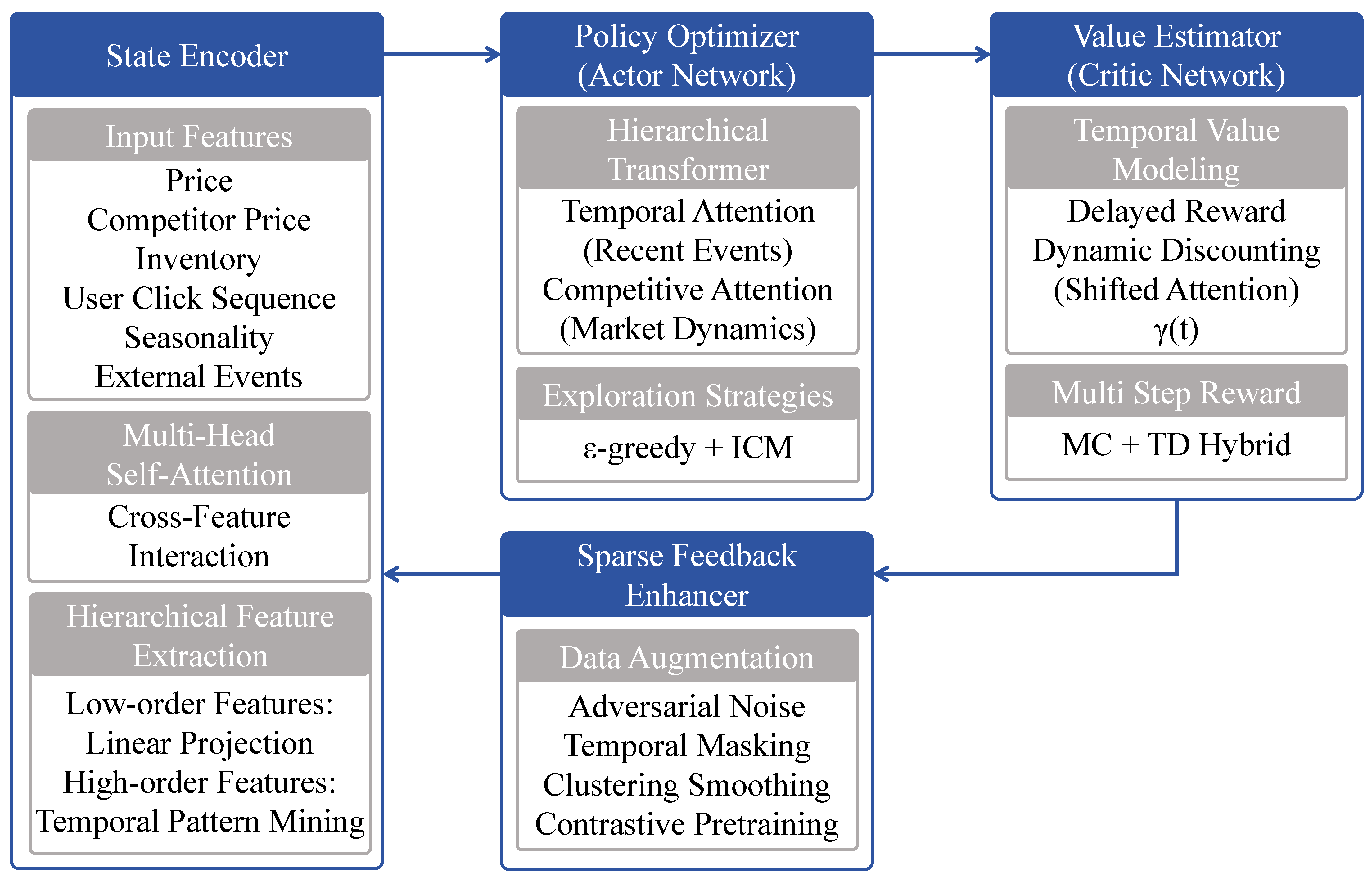
3.3. Proposed Method

A modular DRL strategy-generation system was constructed, in which preprocessed temporal data features were initially processed by a state encoder for multi-level feature extraction. Cross-modal interactions were subsequently realized through multi-head self-attention mechanisms. A strategy optimizer then generated decision actions based on the encoded states, employing an $\epsilon$-greedy strategy combined with an intrinsic motivation mechanism to facilitate exploration. Concurrently, a value estimator modeled future returns based on current states and actions using delayed modeling and dynamic discounting, with training signals optimized via multi-step mixed returns. To enhance feedback robustness, a sparse-enhancement module was introduced, which incorporated adversarial perturbation, temporal masking, and cluster smoothing for structural augmentation and prior training. All modules functioned cooperatively in a closed-loop configuration, enabling efficient generation and dynamic optimization of decision policies under high-dimensional states, as shown in Figure 1 and

Table 2. Layer-wise architecture and parameter count of the proposed method.

Layer	Input Dim	Output Dim	Param
Input Embedding	4	128	512
Positional Encoding	–	128	0
Multi-Head Attention (4 heads)	128	128	49,152
Feed-Forward Network (FFN)	128	128	65,536
LayerNorm × 2	128	128	256
Dropout	–	–	0
GRU-based Value Head	128	1	98,432
Policy Head (MLP)	128	3	384
Total	–	–	214,272

. The overall architecture follows an actor–critic paradigm based on the deep Q-network (DQN) framework. The policy network (actor) generates a stochastic action distribution through a softmax layer, while the value network (critic) estimates the Q-values using a multi-step return formulation. This design combines the sample efficiency and convergence stability of value-based learning with the flexibility of gradient-based policy optimization.

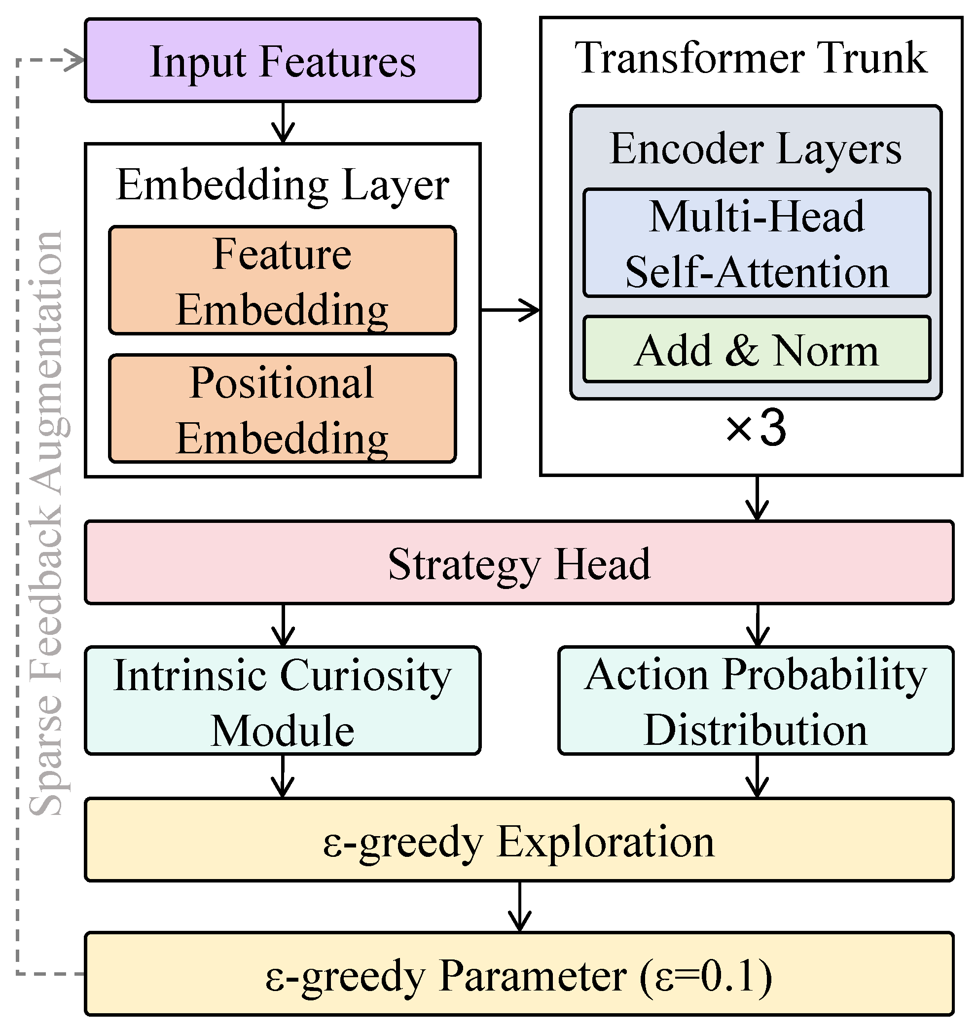
3.3.1. Policy-Learning Module

The policy-learning module represents the core component of the proposed DRL-based pricing-strategy framework, responsible for mapping high-dimensional economic state inputs to distributions over pricing actions. The entire process can be abstractly formulated by the following mathematical expression:

$${\pi }^{\ast }=arg\underset{\pi }{max}{\mathbb{E}}_{\pi }\left[\sum _{t=0}^{\infty }{\gamma }^t{r}_t\right]$$

(17)

Here, ${\pi }^{\ast }$ denotes the optimal pricing policy, and $\pi (a_t|s_t)$ represents the policy function, which outputs a probability distribution over actions $a_t$ given the state $s_t$. The state $s_t$ comprises the current price $p_t$, competitor pricing, user click sequences, inventory levels $I_t$, seasonal factors, and external events. The action $a_t$ refers to the pricing decision made by the platform at time t. The immediate reward $r_t$ is defined as follows:

$$r_t={\lambda }_1·{\mathrm{Profit}}_t+{\lambda }_2·{\mathrm{SalesGrowth}}_t+{\lambda }_3·{\mathrm{StabilityPenalty}}_t$$

(18)

In this formulation, ${\mathrm{Profit}}_t$ denotes the actual profit at time t, ${\mathrm{SalesGrowth}}_t$ measures the relative increase in sales volume compared to a historical average, and ${\mathrm{StabilityPenalty}}_t$ penalizes abrupt pricing fluctuations to encourage smooth strategy evolution. The weighting coefficients are set as ${\lambda }_1=0.6$, ${\lambda }_2=0.3$, and ${\lambda }_3=0.1$, emphasizing a profit-oriented optimization objective while incorporating considerations for sales growth and pricing stability. The learned mapping function from state to action distribution $\pi \theta (a_t|s_t)$ guides the platform in selecting optimal pricing strategies at each time step. The input features of this module include current product prices, competitor prices, inventory levels, user click-behavior sequences, seasonality factors, and external event variables. These features are vectorized via an embedding layer and fused with positional embeddings to retain both sequential and structural information within the transformer backbone network. The embedded state tensor $X\in {\mathbb{R}}^{T\times d}$, where T denotes the sequence length and d is the embedding dimension, is processed through multiple transformer encoder layers for state representation modeling, as shown in Figure 2.

The transformer trunk is composed of three stacked encoder layers, each consisting of a multi-head self-attention mechanism and a feed-forward network, both integrated with residual connections and layer normalization (Add and Norm). In each self-attention layer, the input X is projected into queries (Q), keys (K), and values (V), and the attention weight matrix is computed as $A=\mathrm{softmax}(Q{K}^{\top }/\sqrt{d_k})$. The contextual representation is then obtained via $AV$, followed by multi-head concatenation and a linear projection to yield the fused feature representation. This design enables the policy network to capture intricate dependencies between heterogeneous features such as price trends, user engagement, and competitive actions, which is particularly suitable for economic behavior modeling scenarios characterized by complex causal structures and market dynamics. For instance, the mechanism can emphasize recent user behavior spikes during promotional periods or prioritize inventory fluctuations when supply constraints emerge. Following the transformer backbone, the output features are passed to the strategy head to generate action probabilities. A fully connected layer maps the hidden states to a probability distribution over the pricing action space, denoted as ${\pi }_{\theta }(a|s)$, with the softmax function ensuring proper probability constraints. Specifically, given the state representation $h_t$ at time t, the policy function is defined as ${\pi }_{\theta }(a_t|s_t)=\mathrm{softmax}(W{h}_t+b)$, where W and b are trainable parameters. The resulting probability distribution is used to sample a pricing action $a_t$, which is then passed into the environment for interaction. To enhance exploration capabilities and generalizability, the policy-output stage incorporates an $\epsilon$-greedy strategy and an intrinsic curiosity module (ICM). In the $\epsilon$-greedy strategy, the action with the highest probability $a^{\ast }=arg{max}_a{\pi }_{\theta }(a|s)$ is selected with probability $1-\epsilon$, while a random action is selected with probability $\epsilon$, with $\epsilon =0.1$ in the experiments. The ICM further defines an intrinsic reward $r^{\mathrm{int}}t=||\widehat{\varphi }\left(s_{t+1}^{\ast }\right)-\varphi \left(s_{t+1}\right){||}^2$ based on the prediction error between state–action pairs, thereby encouraging exploration in underrepresented regions of the state space and alleviating policy degradation caused by sparsity in economic behavior data. This design of the policy-learning module offers several mathematical advantages. First, the transformer-based state modeling process is equivalent to constructing a class of learnable dynamic feature kernel functions $K(s_i,s_j)$ within the state space, where the self-attention mechanism adaptively adjusts the weight distribution among features, significantly outperforming fixed-structure convolutional or recurrent units. Second, the multi-head mechanism enables the parallel modeling of local and global dependencies across multiple subspaces, enhancing the policy’s sensitivity to complex market dynamics such as promotional events and seasonal fluctuations. Moreover, the probabilistic output of the policy, combined with the $\epsilon$-greedy exploration mechanism, provides interpretable and elastic action selection, theoretically mitigating the risk of converging to suboptimal local solutions.

3.3.2. Reward Estimation Module

The reward estimation module, serving as the core component for value evaluation in reinforcement learning, is responsible for estimating the contribution of each pricing action to long-term returns. Given that feedback in real-world platforms is often significantly delayed, sparse, and incomplete, a reward-modeling structure integrating multi-step return and dynamic discounting has been designed to enhance both the accuracy of return estimation and the stability of training. Architecturally, the reward estimation module adopts a multi-layer, one-dimensional convolutional neural network (1D-CNN) tailored for temporal modeling, which is motivated by the need to capture local temporal dependencies (e.g., short-term revenue trends or clustered sales fluctuations) in reward sequences with lower computational overhead. The input consists of the state representation vectors from the policy-learning module (i.e., the transformer output), shaped as $(B,T,d)$, where B denotes the batch size, T is the temporal window length, and $d=256$ is the feature dimension. The first convolutional layer employs a kernel size of $k=3$ with $C_1=128$ channels, resulting in an output dimension of $(B,T-2,128)$; the second layer uses a kernel size of $k=3$ with $C_2=64$ channels, yielding $(B,T-4,64)$. A global average pooling layer compresses the temporal dimension into a single vector. This is followed by two fully connected layers with widths of 128 and 1, respectively, producing the value estimate $Q(s_t,a_t)$ for each state–action pair. This structure is not only computationally lightweight but also enhances local dependency modeling among adjacent states through the sliding nature of convolution kernels. From a modeling perspective, the objective function of this module is based on a hybrid multi-step return, which combines Monte Carlo return and temporal difference return through weighted fusion. The learning objective is to minimize the Bellman error as follows:

$${\mathcal{L}}_{\mathrm{value}}={\mathbb{E}}_{(s_t,a_t,r_t,\dots )}\left[{\left(Q(s_t,a_t)-R_t^{\left(n\right)}\right)}^2\right],$$

(19)

where n denotes the number of backward steps and $R_t^{\left(n\right)}$ represents the n-step cumulative return, defined as

$$R_t^{\left(n\right)}=\sum _{i=0}^{n-1}{\gamma }^i{r}_{t+i}+{\gamma }^n·\underset{a^{\prime }}{max}Q(s_{t+n},a^{\prime };{\theta }^{-}),$$

(20)

where $\gamma$ denotes the dynamic discount factor, which is designed as a time-decaying function:

$$\gamma \left(t\right)={\gamma }_0·exp(-\lambda t).$$

(21)

This formulation allows the model to assign moderate but diminishing attention to long-term rewards, thereby balancing short-term and long-term strategy optimization. In experiments, ${\gamma }_0$ is set to $0.99$ and $\lambda$ to $0.01$, which have been empirically determined to be optimal. This module is jointly trained with the policy-learning module, forming an actor–critic architecture. The policy network ${\pi }_{\theta }$ outputs pricing actions, while the value network $Q_{\varphi }$ estimates the returns for those actions under given states. The total loss function used for joint optimization is

$${\mathcal{L}}_{\mathrm{total}}={\mathcal{L}}_{\mathrm{policy}}+\beta ·{\mathcal{L}}_{\mathrm{value}},$$

(22)

where $\beta$ is the weighting coefficient for value loss, which is set to $0.5$ to maintain a balance between policy learning and value estimation. The policy loss ${\mathcal{L}}_{\mathrm{policy}}$ is defined as the cross-entropy between predicted and high-reward actions, encouraging the network to prefer actions with higher expected returns. This reward estimation module offers several advantages in the pricing task. First, the convolutional structure demonstrates strong capabilities in modeling local behavior sequences, which aligns well with the needs of e-commerce pricing scenarios characterized by high correlation and low latency. Second, the use of multi-step returns mitigates the high variance of single-step temporal difference methods and the high bias of full-trajectory returns, achieving a favorable bias–variance trade-off. Third, the introduction of dynamic discounting enables the model to adapt to varying time scales, thereby enhancing generalization capabilities. Mathematically, this module also satisfies the expected convergence properties. When the learning rate $\alpha \to 0$ and $n\to \infty$, the following convergence holds:

$$\underset{n\to \infty }{lim}\mathbb{E}\left[R_t^{\left(n\right)}\right]=\mathbb{E}\left[\sum _{i=0}^{\infty }{\gamma }^i{r}_{t+i}\right].$$

(23)

This implies that the module’s estimation of long-term cumulative rewards asymptotically approaches the expected return in the true environment, ensuring that policy optimization is guided by reliable value signals rather than noise.

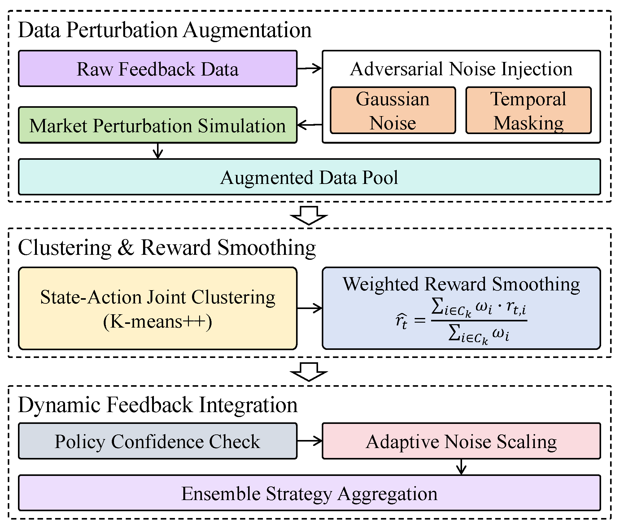
3.3.3. Sparse-Feedback-Enhancement Module

In large-scale data environments, behavioral feedback often exhibits high levels of sparsity and heterogeneity, particularly under conditions in which data recording is constrained by uneven user attention, short sampling intervals, or asynchronous event timing. These factors frequently result in missing or delayed supervisory signals, which can significantly undermine the accuracy of value estimation during training, amplify gradient propagation errors, and ultimately lead to policy degradation or convergence to suboptimal solutions. This issue critically impairs the model’s generalization and stability in complex environments. To address this, a sparse-feedback-enhancement module (reward denoising module) has been designed to improve robustness, generalizability, and exploratory capabilities under sparse-feedback conditions. This module integrates data perturbation augmentation, temporal masking, state–action clustering, and weighted return smoothing as core mechanisms, as shown in Figure 3.

The first component, data perturbation augmentation, includes adversarial noise injection and Gaussian noise perturbation to simulate uncertainty in market feedback by generating perturbed samples. Adversarial noise is computed using the Fast Gradient Sign Method (FGSM), applying perturbation $\delta =ϵ·\mathrm{sign}\left({\nabla }_x\mathcal{L}\right)$ to the input state features x, thereby yielding perturbed samples $x^{\prime }=x+\delta$. Gaussian noise sampled from $\mathcal{N}(0,{\sigma }^2)$ is added to critical variables such as price and inventory to generate boundary-near training instances. To further enhance robustness to partial temporal observation, a temporal masking mechanism is employed, randomly masking a proportion of time steps t in the state sequence. This forces the model to infer action values from incomplete observations, thereby improving tolerance to missing data. The second component, clustering and reward smoothing, performs joint clustering of high-dimensional state–action pairs $(s_t,a_t)$ using the K-means++ algorithm. Within each cluster $C_i$, a weighted average reward ${\tilde{r}}_t$ is constructed as the smoothed feedback signal, calculated as

$$\tilde{r}t={\displaystyle \frac{\sum j\in \mathcal{N}\left(t\right){\omega }_j{r}_j}{{\sum }_{j\in \mathcal{N}\left(t\right)}{\omega }_j}},$$

(24)

where $\mathcal{N}\left(t\right)$ denotes the KNN of $(s_t,a_t)$ in the embedding space and ${\omega }_j$ is a distance-based weight defined by ${\omega }_j=exp(-\alpha |z_t-z_j{|}^2)$, where $z_t$ is the embedding of the state and $\alpha$ is a decay coefficient. A policy confidence check mechanism is further incorporated, executing smoothing only when the output confidence $\pi (a_t|s_t)$ exceeds a predefined threshold, preventing over-reliance on noisy data during early exploration stages and preserving training validity. During training, the original reward $r_t$ is fused with the smoothed reward ${\tilde{r}}_t$ to form an enhanced reward signal $r_t^{\mathrm{aug}}$, computed as

$$r_t^{\mathrm{aug}}=\lambda ·r_t+(1-\lambda )·{\tilde{r}}_t.$$

(25)

The weighting coefficient $\lambda \in [0,1]$ is adaptively adjusted based on the clustering density, confidence, and loss dynamics. A higher weight is assigned to ${\tilde{r}}_t$ in regions of high density and low confidence to mitigate bias introduced by skewed samples. Additionally, an ensemble strategy aggregation mechanism is introduced to improve generalization, whereby policy outputs under multiple perturbation and clustering instances are aggregated through behavior–consistency weighting. This yields a more robust policy estimation and prevents training drift caused by individual perturbations. Mathematically, this smoothing process is analogous to applying a low-pass filter to the reward function, suppressing high-frequency noise while preserving stable local value signals. In reinforcement learning, this reduces the variance of value-error propagation. Theoretically, for perturbed feedback $r_t^{\prime }=r_t+{ϵ}_t$, where ${ϵ}_t$ is independent and identically distributed with zero mean, the following holds after smoothing:

$$\mathbb{E}[{\tilde{r}}_t]=\mathbb{E}[r_t],\mathrm{Var}[{\tilde{r}}_t]<\mathrm{Var}[r_t^{\prime }].$$

(26)

This result indicates that the smoothed reward remains an unbiased estimator while achieving variance reduction, thereby enhancing the stability of Q-value estimation and driving the policy network toward a superior convergence solution.

4. Results and Discussion

4.1. Experimental Setup and Evaluation Metrics

4.1.1. Hardware and Software Platform

In the present study, the choice of hardware platform plays a critical role in the training and execution of DRL models. To ensure efficient training on large-scale datasets, high-performance computing resources were employed. Specifically, multiple servers equipped with NVIDIA Tesla V100 GPUs (manufactured by NVIDIA Corporation, headquartered in Santa Clara, CA, USA) were utilized, offering substantial parallel computing capabilities that significantly accelerate the training of deep learning algorithms. These servers are further supported by the latest Intel Xeon processors (manufactured by Intel Corporation, headquartered in Santa Clara, CA, USA), ensuring stable and efficient CPU–GPU cooperation during data preprocessing, model training, and results analysis. Each server is outfitted with 128 GB of DDR4 RAM (manufactured by Intel Corporation, headquartered in Santa Clara, CA, USA) to accommodate the loading and processing of large volumes of data. In addition, NVMe SSDs (manufactured by Intel Corporation, headquartered in Santa Clara, CA, USA) were used for storage to facilitate fast data reading and writing. This hardware configuration allows the DRL algorithms to iterate rapidly, greatly reducing training time and improving experimental efficiency. On the software side, Python was selected as the primary programming language, combined with the TensorFlow framework, for implementing DRL models. TensorFlow, one of the most widely used deep learning frameworks, supports GPU acceleration and enables efficient training of large-scale neural networks. Its flexibility and scalability allow for the implementation of various models and algorithms. For reinforcement learning environment interaction, the OpenAI Gym platform was employed as the training and testing environment. OpenAI Gym provides a collection of standardized, modular environments suitable for various reinforcement learning algorithms, facilitating seamless integration between agents and environments. Additionally, Pandas and NumPy were used for data cleaning, manipulation, and analysis. All experiments were conducted on the Ubuntu 20.04 Linux operating system, ensuring platform stability and compatibility. This comprehensive hardware and software setup ensures efficient execution and guarantees the reliability and accuracy of the experimental results.

4.1.2. Hyperparameter Settings

To ensure generalizability and stability, the dataset was divided using a temporal split strategy to prevent future information leakage inherent in standard random cross-validation schemes. Specifically, data collected from January to September 2023 were used for training, while data from October to December 2023 were reserved for testing. This setup simulates real-world deployment scenarios in which pricing strategies must generalize to future unseen market conditions. In addition, since the four behavior data subsets (i.e., browsing behavior, inventory status, product pricing records, and sales feedback) span different temporal ranges, each subset was treated as an independent experimental task. For each task, training and testing splits were performed within the respective subset’s available time range (e.g., browsing data from January–June were split into training on January–May and testing on June), thereby ensuring consistency in temporal ordering and eliminating the risk of information leakage over time. Several hyperparameters were configured to ensure effective training and convergence of the DRL model. The learning rate $\alpha$ was set to 0.001, a value determined through empirical tuning to balance training speed and convergence stability. The discount factor $\gamma$ was set to 0.99, reflecting a strong emphasis on long-term rewards and improving the stability and accuracy of pricing policies. The experience replay buffer size was configured to store 100,000 samples to ensure a rich and diverse history of interactions. A batch size of 64 was selected to balance computational efficiency and learning diversity across different states. The neural network architecture adopted in the deep Q-network (DQN) consisted of three fully connected layers, each containing 256 neurons. The ReLU activation function was applied to each layer to enhance the model’s capacity for nonlinear representation. The target network was updated every 10,000 steps during training to stabilize learning.

4.1.3. Evaluation Metrics

The performance of the model was assessed using several key evaluation metrics, including total profit gain, average reward, strategy stability (standard deviation of actions), the coefficient of determination ($R^2$) for the reward–price relationship, the Sharpe ratio, and maximum drawdown.

$$\mathrm{Total}\mathrm{Profit}\mathrm{Gain}={\displaystyle \frac{P_{\mathrm{final}}-P_{\mathrm{initial}}}{P_{\mathrm{initial}}}}\times 100\%$$

(27)

$$\mathrm{Average}\mathrm{Reward}={\displaystyle \frac{1}{N_1}}\sum _{t=1}^{N_1}{r}_t$$

(28)

$$\mathrm{Std}.\mathrm{of}\mathrm{Actions}=\sqrt{{\displaystyle \frac{1}{N_1}}\sum _{t=1}^{N_1}{(a_t-\overline{a})}^2}$$

(29)

$$R^2=1-{\displaystyle \frac{{\sum }_{t=1}^{N_2}{(r_t-{\widehat{r}}_t)}^2}{{\sum }_{t=1}^{N_2}{(r_t-\overline{r})}^2}},$$

(30)

$$\mathrm{Sharpe}\mathrm{Ratio}={\displaystyle \frac{\overline{r}-r_f}{{\sigma }_r}}$$

(31)

$$\mathrm{Max}\mathrm{Drawdown}=\underset{t\in [1,T]}{max}\left({\displaystyle \frac{{max}_{\tau \in [1,t]}{P}_{\tau }-P_t}{{max}_{\tau \in [1,t]}{P}_{\tau }}}\right)$$

(32)

where $P_{\mathrm{final}}$ represents the total profit obtained by the model at the end of training and $P_{\mathrm{initial}}$ is the total profit at the initial state. The variable $r_t$ denotes the immediate reward at time t, $N_1$ is the total number of training steps, $a_t$ refers to the action taken at time t, and $\overline{a}$ is the average of all actions taken. In addition, ${\widehat{r}}_t$ is the model’s predicted reward, $\overline{r}$ is the mean of the actual rewards, and $N_2$ is the total number of data points. $r_f$ is the baseline risk-free reward (set to 0 in our experiments for simplicity), and ${\sigma }_r$ is the standard deviation of the reward sequence. $P_t$ denotes the cumulative profit at time t. The total profit gain measures the percentage increase in the cumulative profit achieved through the optimized pricing policy relative to the initial profit level. The average reward quantifies the mean reward obtained per decision step, reflecting the effectiveness of the learned strategy throughout the training process. Strategy stability, represented by the standard deviation of actions, evaluates the consistency of the pricing decisions, particularly under changing market conditions. The $R^2$ metric assesses the correlation between the predicted pricing strategies and actual revenue, where higher $R^2$ values indicate a stronger alignment between the model’s pricing outputs and real-world revenue patterns. The Sharpe ratio measures the average excess reward earned per unit of reward volatility, indicating the risk-adjusted efficiency of the pricing strategy throughout the decision-making process. And the maximum drawdown quantifies the worst-case decline from a historical peak in the cumulative profit, reflecting the extent of the short-term loss risk encountered during strategy execution.

4.2. Comparative Experiments and Baselines

In order to evaluate the performance of the proposed method, several baseline models were considered for comparison. These included XGBoost [61], DQN [62], BERT [63], transformer-based prediction market models [64], and LSTM-based prediction market models [65]. Each of these baselines represents a different approach to pricing optimization, enabling a comprehensive comparison across various state-of-the-art techniques. XGBoost (Extreme Gradient Boosting) is a highly effective implementation of gradient-boosted decision trees and is widely used for supervised learning tasks. It has been particularly successful in many machine learning competitions due to its scalability, efficiency, and ability to handle various types of data. The deep Q-network (DQN) is another baseline model used for reinforcement learning tasks, particularly in the context of dynamic pricing. The DQN model approximates the Q-value function using a deep neural network, allowing the model to learn optimal pricing strategies by interacting with the environment. BERT (Bidirectional Encoder Representations from Transformers) is a pre-trained transformer-based model that has achieved significant success in natural language processing tasks. BERT models are able to understand contextual relationships between words in a text by training on large corpora with both left-to-right and right-to-left contexts. The transformer-based prediction market model employs self-attention mechanisms to capture dependencies across various market conditions and consumer behavior. By using multi-head attention layers, the transformer model learns the relationships between market inputs and predictions, allowing it to make more accurate forecasts over long sequences. The LSTM-based prediction market model is another baseline used to model sequential dependencies, especially in time-series data such as sales and pricing history. LSTM is well known for handling long-range dependencies by using gating mechanisms that control the flow of information.

4.3. Results and Analysis

4.3.1. Experimental Results of Different Pricing-Strategy Models

This experiment was designed to evaluate the overall capability of various models to predict pricing strategies under large-scale heterogeneous behavior data. Particular attention was given to their performance in terms of profit growth, behavioral stability, and the consistency of strategy responses, as shown in

Table 3. Experimental results of different pricing-strategy models.

Model	Total Profit Gain	Average Reward	Std. of Actions	${\mathbf{R}}^2$	Sharpe Ratio	Max Drawdown
XGBoost [61]	0.12	3.25	0.97	0.61	0.64	0.43
BERT [63]	0.17	3.56	0.89	0.68	0.68	0.39
LSTM-based [65]	0.21	3.72	0.85	0.72	0.72	0.36
Transformer-based [64]	0.24	4.01	0.79	0.77	0.77	0.33
DQN [62]	0.28	4.23	0.66	0.80	0.80	0.28
Proposed method	0.34	4.78	0.41	0.88	0.86	0.21

and Figure 4.

The results indicate that XGBoost demonstrated the weakest performance across all metrics, primarily due to its static modeling approach, which failed to capture the temporal dynamics inherent in complex behavioral feedback. While BERT exhibited some capability in modeling sequential data, its contextual embedding mechanism struggled to generate stable policies in the absence of reinforcement signals. The LSTM-based model performed better in handling continuous time series but still suffered from degradation in capturing long-term dependencies. The transformer-based model significantly improved the efficiency and stability of policy learning through its global attention mechanism. The DQN model, equipped with a reinforcement learning structure, adapted policies dynamically and performed well in terms of average return and behavioral smoothness. The proposed method achieved the best results across all evaluation metrics, which can be attributed to its structural design that accommodates the entire modeling pipeline of multi-source behavior data. From a mathematical perspective, the multi-head attention mechanism of the transformer effectively captured long-range dependencies, the delayed-reward estimation module enhanced sensitivity to future gains, and the sparse-feedback-enhancement mechanism mitigated training bias caused by low-frequency behavioral samples. The strategy-generation process incorporated dynamic exploration and value-constrained mechanisms, theoretically constructing a more stable convergence path toward the optimal solution. As a result, the framework succeeded in simultaneously achieving profit maximization and smooth responses under complex behavioral environments.

4.3.2. Performance Evaluation on Different Subsets of Economic Behavior Data

This experiment was designed to evaluate the generalization capability and response stability of different models when applied to various dimensions of economic behavior data in a large-scale setting. By constructing four specialized subsets—product pricing records, sales feedback, browsing behavior, and inventory status—the performance of each model under different types of information structures was assessed to determine its adaptability and prediction effectiveness.

As shown in

Table 4. Prediction results on product pricing records dataset.

Model	Total Profit Gain	Average Reward	Std. of Actions	${\mathbf{R}}^2$	Sharpe Ratio	Max Drawdown
XGBoost [61]	0.13	3.38	0.92	0.62	0.65	0.41
BERT [63]	0.17	3.67	0.86	0.69	0.69	0.37
LSTM-based [65]	0.20	3.88	0.79	0.73	0.73	0.34
Transformer-based [64]	0.24	4.09	0.73	0.78	0.78	0.31
DQN [62]	0.28	4.33	0.61	0.82	0.81	0.27
Proposed method	0.36	4.91	0.38	0.90	0.87	0.19

,

Table 5. Prediction results on sales feedback dataset.

Model	Total Profit Gain	Average Reward	Std. of Actions	${\mathbf{R}}^2$	Sharpe Ratio	Max Drawdown
XGBoost [61]	0.12	3.31	0.94	0.60	0.63	0.44
BERT [63]	0.16	3.62	0.87	0.67	0.67	0.39
LSTM-based [65]	0.22	3.91	0.78	0.74	0.74	0.33
Transformer-based [64]	0.25	4.13	0.72	0.78	0.78	0.30
DQN [62]	0.29	4.36	0.60	0.83	0.82	0.25
Proposed method	0.37	4.85	0.37	0.91	0.89	0.18

,

Table 6. Prediction results on browsing behavior dataset.

Model	Total Profit Gain	Average Reward	Std. of Actions	${\mathbf{R}}^2$	Sharpe Ratio	Max Drawdown
XGBoost [61]	0.14	3.41	0.90	0.63	0.66	0.42
BERT [63]	0.18	3.71	0.85	0.70	0.70	0.38
LSTM-based [65]	0.21	3.93	0.77	0.74	0.74	0.35
Transformer-based [64]	0.25	4.07	0.70	0.79	0.79	0.29
DQN [62]	0.29	4.26	0.60	0.83	0.82	0.26
Proposed method	0.33	4.66	0.43	0.87	0.85	0.20

and

Table 7. Prediction results on inventory status dataset.

Model	Total Profit Gain	Average Reward	Std. of Actions	${\mathbf{R}}^2$	Sharpe Ratio	Max Drawdown
XGBoost [61]	0.15	3.43	0.93	0.64	0.67	0.40
BERT [63]	0.19	3.74	0.84	0.69	0.70	0.36
LSTM-based [65]	0.23	3.96	0.75	0.75	0.75	0.32
Transformer-based [64]	0.26	4.11	0.67	0.78	0.79	0.28
DQN [62]	0.30	4.30	0.55	0.82	0.81	0.24
Proposed Method	0.32	4.72	0.44	0.86	0.84	0.22

and Figure 5, the proposed method consistently outperformed all baselines across the sub-tasks. It achieved the highest total profit gain and average reward on the sales feedback dataset while maintaining lower action variability and higher correlation scores in the browsing behavior and inventory status datasets, demonstrating strong robustness in handling unstructured behavior data. From a theoretical standpoint, XGBoost, although capable of modeling structured features, lacked the temporal representation and contextual modeling abilities necessary for sequential prediction, resulting in the weakest performance across all subsets. BERT captured semantic relationships to a certain extent, but the inconsistency between its pretraining objectives and temporal dynamics hindered its sequential adaptability. The LSTM-based model benefited from its recurrent architecture for learning local dependencies but suffered from memory decay when modeling long-range behavioral cycles. In contrast, the transformer-based model leveraged its global attention mechanism to model nonlinear dependencies over extended time horizons, resulting in performance improvements. The DQN model constructed an iterative optimization path via reinforcement learning, providing advantages in sparse-feedback environments. The proposed method, which combines multi-head attention structures, delayed-return estimation, and sparse-feedback enhancement, achieved synergistic improvements in representation learning, value estimation, and policy stability, thereby enhancing prediction accuracy and consistency across heterogeneous behavior data subsets.

4.3.3. Ablation Study of Key Modules in the Proposed Method

This experiment was conducted to assess the individual contributions of the key structural components within the overall strategy-generation framework by progressively removing each module.

As shown in

Table 8. Ablation study of key modules in the proposed method.

Configuration	Total Profit Gain	Average Reward	Std. of Actions	${\mathbf{R}}^2$	Sharpe Ratio	Max Drawdown
w/o All (Only Backbone)	0.19	3.42	0.91	0.65	0.66	0.45
w/o Perturbation	0.23	3.88	0.75	0.72	0.72	0.37
w/o Profit Backtracking	0.26	4.10	0.68	0.77	0.76	0.32
w/o Strategy Stabilizer	0.29	4.21	0.57	0.80	0.80	0.27
Proposed (Full Model)	0.34	4.78	0.41	0.88	0.86	0.21

, a continuous improvement across all four metrics was observed as individual components were incrementally restored, demonstrating the synergistic value of each module in modeling complex behavioral patterns under large-scale data conditions. In the absence of the perturbation module, the model’s adaptability to dynamic behavior changes declined significantly. When the profit-backtracking module was removed, the ability to capture long-term rewards was diminished, leading to reduced prediction accuracy and lower cumulative returns. Disabling the strategy stabilizer resulted in a notable increase in policy variance, compromising the consistency of execution. The full model consistently outperformed all ablated configurations, confirming the compounded benefit of combining all modules. From a theoretical perspective, although the backbone structure possessed basic temporal awareness and action-mapping capabilities, it lacked the mechanisms required to effectively address data sparsity and delayed feedback. The perturbation module introduced Gaussian and adversarial noise mechanisms, thereby constructing a localized generalization neighborhood within the input space to enhance policy robustness. The profit-backtracking module employs a multi-step bootstrapped return formulation defined as

$$R_t^{\left(n\right)}=\sum _{i=0}^{n-1}{\gamma }^i{r}_{t+i}+{\gamma }^n\underset{a^{\prime }}{max}Q(s_{t+n},a^{\prime })$$

(33)

where n is the lookahead step (set to $n=5$ in our experiments), $\gamma$ is the discount factor, and $Q(s,a)$ is the estimated action-value function. This approach allowed the model to improve value-function accuracy, enabling it to optimize policy trajectories under long-term incentive structures. The strategy stabilizer reweighted historical action distributions to impose structural constraints in the output space, reducing volatility and enhancing policy coherence. Together, these modules jointly optimized the convergence trajectory from the input perturbation to value estimation and action generation, achieving the dual objectives of improved stability and increased return from a mathematical standpoint.

4.3.4. Cross-Stock Domain Transfer Evaluation

To evaluate the model’s generalization ability across different assets within the same market domain, a domain transfer experiment was conducted. The agent was trained exclusively on AAPL stock data and directly evaluated on MSFT data without any fine-tuning. All features and preprocessing procedures were kept consistent. The evaluation metrics included the total profit gain, average reward, policy stability, $R^2$ correlation, and Sharpe ratio.

Table 9. Cross-stock generalization performance: training on AAPL, testing on MSFT.

Model	Total Profit Gain	Average Reward	Std. of Actions	R2 Score	Sharpe Ratio
XGBoost	0.08	2.91	1.03	0.52	0.64
LSTM-based	0.14	3.45	0.84	0.67	0.71
Transformer-based	0.18	3.88	0.74	0.75	0.76
DQN	0.21	4.01	0.60	0.78	0.79
Proposed	0.27	4.49	0.42	0.85	0.83

summarizes the performance of various models under this cross-stock generalization scenario.

The results demonstrate that the proposed method achieved superior cross-stock generalization performance. Despite being trained on AAPL, the model exhibited a high $R^2$ score (0.85) and low action standard deviation (0.42) when deployed on MSFT, indicating consistent policy stability and accurate reward prediction. This supports the model’s capability to generalize across assets within the same market domain without fine-tuning.

4.4. Discussion

4.4.1. Empirical Findings and Behavioral Insights

A series of experiments was conducted to systematically evaluate the proposed model from three perspectives: overall performance, module contributions, and robustness across different subsets of behavior data. The results demonstrated that the proposed framework exhibits strong adaptability, stability, and generalization capabilities under complex economic behavioral scenarios. In real-world applications, platform-level decision-making is often challenged by high-dimensional heterogeneity, delayed feedback, and volatile user behavior. Traditional static or shallow learning models fail to effectively integrate such multi-source, heterogeneous information. The proposed approach, constructed and validated on large-scale daily-granularity behavior data from e-commerce platforms, exhibits practical potential for deployment. In terms of overall performance, the proposed strategy-generation framework significantly outperformed mainstream models such as XGBoost, BERT, LSTM, transformer, and standard DQN across all metrics, including total profit gain, average reward, behavioral output stability, and profit–price curve fitting. In the dataset collected throughout 2023 from jd.com, taobao.com, suning.com, and vip.com, numerous occurrences, such as temporary promotions, unexpected demand surges, and inventory fluctuations, were observed. These patterns require models with strong temporal sensitivity and adaptive policy adjustment capabilities. Unlike traditional methods that tend to respond prematurely or belatedly due to rigid weighting schemes, the proposed model demonstrated the ability to generate stable, trend-aware policy trajectories in the presence of highly imbalanced and volatile economic signals. For instance, in datasets related to holiday promotions for consumer electronics, the proposed method responded more accurately to changes in click behavior and peak historical sales, maintaining continuity and an upward trajectory in profit outcomes.

Among the four behavior data subsets, the model performed best on sales feedback and pricing records data, indicating a particular sensitivity to features exhibiting numerical continuity and strong price–sales coupling. In the sales feedback subset, the model captured periodic patterns and temporal surges in sales, effectively avoiding policy instability at peak or off-season transitions, which is critical for datasets involving cyclical categories such as food and personal care. Although the performance was slightly lower on the browsing behavior and inventory status datasets, the proposed method still outperformed all baseline models. The browsing dataset, characterized by high uncertainty and weak click–conversion correlation, presented a low signal-to-noise ratio. While the model could not fully predict post-click conversion behavior, the combination of perturbation augmentation and policy stabilization successfully suppressed the influence of behavioral outliers. In inventory modeling, the model estimated potential stockout risks by learning from inventory update frequencies and outbound flow patterns, enabling timely policy adjustments. This feature proved particularly valuable in domains prone to stock discontinuities, such as books and home goods. Regarding module contributions, the ablation study confirmed the distinct value of the three key modules in practical scenarios. The perturbation augmentation module introduced Gaussian and adversarial noise to price shifts, sales fluctuations, and inventory interventions, simulating real-world market uncertainty such as competitor price cuts or temporary policy changes. Without this module, the model’s adaptability diminished, leading to increased policy volatility and overreaction to minor behavioral disturbances. The profit-backtracking module was especially effective in desynchronized sequences, in which platform actions such as pre-event advertisements precede actual revenue realization by several days. By leveraging multi-step discounted returns, the module allowed the early incorporation of anticipated profits, thus enhancing foresight and buffering capacity in policy generation. The strategy stabilizer played a critical role under high-frequency policy update constraints, as operational systems often limit the number of adjustments per day. This module applied weighted reinforcement from historical behavior to smooth the current policy output, effectively controlling fluctuations and enhancing the operational feasibility and responsiveness of platform strategies.

4.4.2. Computational Complexity Analysis

From the perspective of computational efficiency, the proposed framework maintains a favorable balance between model expressiveness and runtime feasibility. The transformer-based policy-learning module, composed of three stacked encoder layers, introduces a self-attention mechanism with a complexity of $\mathcal{O}\left(T^{2}d\right)$, where T denotes the input sequence length and d is the feature embedding dimension. In our setting, $T=10$ and $d=256$, which constrains the quadratic growth and allows practical training on modern GPUs. Multi-head attention introduces a constant multiplicative overhead proportional to the number of heads (set to four in our implementation), but parallelization across heads mitigates latency. The reward estimation module adopts a 1D convolutional architecture with a total of two convolutional layers and one pooling operation. Its time complexity is $\mathcal{O}\left(Tkd\right)$, where k is the kernel size. This design is significantly more efficient than a transformer- or RNN-based critic while still capturing local dependencies through sliding receptive fields. The entire training pipeline runs on a single Tesla V100 GPU (manufactured by NVIDIA Corporation, headquartered in Santa Clara, CA, USA) with approximately 24 min per epoch and peak memory usage below 12 GB, as profiled on the full-scale dataset. Furthermore, the sparse-feedback-enhancement module operates during training only and introduces minimal inference-time overhead. Clustering-based reward smoothing has a complexity of $\mathcal{O}\left(Nk\right)$ for k-nearest neighbor search, where N is the batch size. However, this process is offloaded to auxiliary GPU streams and does not impede forward or backward propagation.

In summary, the overall framework achieves a complexity-efficient configuration that supports deployment in real-time decision-making systems. Compared with other DRL-based pricing models, the proposed approach introduces only moderate computational overhead while yielding consistent gains in stability, generalization, and long-horizon value estimation.

4.5. Limitations and Future Work

Despite the superior performance demonstrated by the proposed strategy-generation and prediction framework across various large-scale behavior data scenarios, several limitations remain that warrant further investigation and refinement. First, the current approach still relies on a minimum amount of historical behavior data to support state modeling and value estimation, which may pose challenges during cold-start phases or in cases involving newly deployed platforms and short-lived product categories. Under such conditions, the stability of early-stage policy training may be insufficient. Second, the model’s training and inference procedures are currently executed within a centralized framework that aggregates data and generates policies in a unified manner. This architecture does not account for data silos and heterogeneity that are common across different platforms. In practical e-commerce environments, significant structural and access discrepancies exist among platforms with respect to data sharing. Future extensions could incorporate federated learning or multi-agent coordination mechanisms to enable cross-platform policy alignment and knowledge sharing without exposing raw data, thereby enhancing deployment flexibility and scalability in real-world settings. Future work will also consider the integration of multimodal information fusion mechanisms. By leveraging graph neural networks or joint language–behavior encoding strategies, diverse modalities—such as textual content, imagery, news feeds, and sequential user behavior—can be modeled collectively. This enhancement is expected to improve the model’s adaptability to complex and dynamic market conditions while increasing its sensitivity to latent strategic signals. Ultimately, such developments would facilitate the construction of an interpretable and practically valuable intelligent optimization system for strategic decision-making.

5. Conclusions

Under the paradigm of data-driven intelligent decision-making, a fundamental challenge has emerged in effectively extracting informative patterns from high-dimensional, heterogeneous, and sparsely labeled economic behavior data and in constructing stable and forward-looking strategy-optimization models. To address the limitations of existing approaches—such as inadequate modeling of long-term returns, high sensitivity to behavioral perturbations, and poor control over policy fluctuations—a DRL framework has been proposed. This framework integrates perturbation-based augmentation, delayed-reward estimation, and policy-stabilization mechanisms for dynamic strategy generation and profit forecasting. The architecture is built upon a transformer backbone, incorporating both policy and value networks. Data diversity is enhanced through the use of perturbation-injected samples, while multi-step return estimation is employed to improve reward perception over extended time horizons. In addition, a behavior-weighted stabilization mechanism is applied to suppress oscillations in policy outputs, thereby improving the model’s responsiveness to complex behavioral dynamics and ensuring output consistency. Extensive experiments were conducted using real-world economic behavior data collected from jd.com, taobao.com, suning.com, and vip.com. The results demonstrated the effectiveness of the proposed method. On the sales feedback subset, the highest total profit gain of 0.37 was achieved, along with an average reward of 4.85, a policy action standard deviation of only 0.37, and a profit-to-price correlation score of $R^2=0.91$. Comparable stability and superior performance were observed on other subsets such as pricing records and inventory status when compared with baseline models. These findings indicate that the proposed framework is capable of effectively handling complex decision-making scenarios characterized by sparse feedback, behavioral heterogeneity, and temporal volatility, thereby offering strong generalization capabilities and significant potential for real-world application.

References

1. Sedliacikova, M.; Moresova, M.; Alac, P.; Drabek, J. How do behavioral aspects affect the financial decisions of managers and the competitiveness of enterprises? J. Compet. 2021, 13, 99–116. [Google Scholar] [CrossRef]
2. Umapathy, T. Behavioral Economics: Understanding Irrationality In Economic Decision-Making. Migr. Lett. 2024, 21, 923–932. [Google Scholar]
3. Zhou, X.; Chen, S.; Ren, Y.; Zhang, Y.; Fu, J.; Fan, D.; Lin, J.; Wang, Q. Atrous Pyramid GAN Segmentation Network for Fish Images with High Performance. Electronics 2022, 11, 911. [Google Scholar] [CrossRef]
4. Das, P.; Pervin, T.; Bhattacharjee, B.; Karim, M.R.; Sultana, N.; Khan, M.S.; Hosien, M.A.; Kamruzzaman, F. Optimizing real-time dynamic pricing strategies in retail and e-commerce using machine learning models. Am. J. Eng. Technol. 2024, 6, 163–177. [Google Scholar] [CrossRef]
5. Alwan, A.A.; Ciupala, M.A.; Brimicombe, A.J.; Ghorashi, S.A.; Baravalle, A.; Falcarin, P. Data quality challenges in large-scale cyber-physical systems: A systematic review. Inf. Syst. 2022, 105, 101951. [Google Scholar] [CrossRef]
6. Yin, C.; Han, J. Dynamic pricing model of e-commerce platforms based on deep reinforcement learning. Comput. Model. Eng. Sci. 2021, 127, 291–307. [Google Scholar] [CrossRef]
7. Izaret, J.M.; Sinha, A. Game Changer: How Strategic Pricing Shapes Businesses, Markets, and Society; John Wiley & Sons: Hoboken, NJ, USA, 2023. [Google Scholar]
8. Zhang, L.; Zhang, Y.; Ma, X. A New Strategy for Tuning ReLUs: Self-Adaptive Linear Units (SALUs). In Proceedings of the ICMLCA 2021; 2nd International Conference on Machine Learning and Computer Application, VDE, Shenyang, China, 17–19 December 2021; pp. 1–8. [Google Scholar]
9. Nagle, T.T.; Müller, G.; Gruyaert, E. The Strategy and Tactics of Pricing: A Guide to Growing More Profitably; Routledge: London, UK, 2023. [Google Scholar]
10. Gast, R.; Solla, S.A.; Kennedy, A. Neural heterogeneity controls computations in spiking neural networks. Proc. Natl. Acad. Sci. USA 2024, 121, e2311885121. [Google Scholar] [CrossRef]
11. Mehrjoo, S.; Amoozad Mahdirji, H.; Heidary Dahoei, J.; Razavi Haji Agha, S.H.; Hosseinzadeh, M. Providing a Robust Dynamic Pricing Model and Comparing It with Static Pricing in Multi-level Supply Chains Using a Game Theory Approach. Ind. Manag. J. 2023, 15, 534–565. [Google Scholar]
12. Jalota, D.; Ye, Y. Stochastic online fisher markets: Static pricing limits and adaptive enhancements. Oper. Res. 2025, 73, 798–818. [Google Scholar] [CrossRef]
13. Cohen, M.C.; Miao, S.; Wang, Y. Dynamic pricing with fairness constraints. SSRN 2021, 09, 3930622. [Google Scholar] [CrossRef]
14. Sari, E.I.P.; Aurachman, R.; Akbar, M.D. Determination Price Ticket Of Airline Low-cost Carrier Based On Dynamic Pricing Strategy Using Multiple Regression Method. eProceedings Eng. 2021, 8, 6881–6892. [Google Scholar]
15. Skiera, B.; Reiner, J.; Albers, S. Regression analysis. In Handbook of Market Research; Springer: Berlin/Heidelberg, Germany, 2021; pp. 299–327. [Google Scholar]
16. Li, Q.; Ren, J.; Zhang, Y.; Song, C.; Liao, Y.; Zhang, Y. Privacy-Preserving DNN Training with Prefetched Meta-Keys on Heterogeneous Neural Network Accelerators. In Proceedings of the 2023 60th ACM/IEEE Design Automation Conference (DAC), San Francisco, CA, USA, 9–13 July 2023; pp. 1–6. [Google Scholar]
17. Anis, H.T.; Kwon, R.H. A sparse regression and neural network approach for financial factor modeling. Appl. Soft Comput. 2021, 113, 107983. [Google Scholar] [CrossRef]
18. Li, Q.; Zhang, Y.; Ren, J.; Li, Q.; Zhang, Y. You Can Use But Cannot Recognize: Preserving Visual Privacy in Deep Neural Networks. arXiv 2024, arXiv:2404.04098. [Google Scholar]
19. Li, D.; Xin, J. Deep learning-driven intelligent pricing model in retail: From sales forecasting to dynamic price optimization. Soft Comput. 2024, 28, 12281–12297. [Google Scholar] [CrossRef]
20. Chuang, Y.C.; Chiu, W.Y. Deep reinforcement learning based pricing strategy of aggregators considering renewable energy. IEEE Trans. Emerg. Top. Comput. Intell. 2021, 6, 499–508. [Google Scholar] [CrossRef]
21. Li, Q.; Zhang, Y. Confidential Federated Learning for Heterogeneous Platforms against Client-Side Privacy Leakages. In Proceedings of the ACM Turing Award Celebration Conference, Changsha, China, 5–7 July 2024; pp. 239–241. [Google Scholar]
22. Massahi, M.; Mahootchi, M. A deep Q-learning based algorithmic trading system for commodity futures markets. Expert Syst. Appl. 2024, 237, 121711. [Google Scholar] [CrossRef]
23. Park, M.; Kim, J.; Enke, D. A novel trading system for the stock market using Deep Q-Network action and instance selection. Expert Syst. Appl. 2024, 257, 125043. [Google Scholar] [CrossRef]
24. Liang, Y.; Hu, Y.; Luo, D.; Zhu, Q.; Chen, Q.; Wang, C. Distributed Dynamic Pricing Strategy Based on Deep Reinforcement Learning Approach in a Presale Mechanism. Sustainability 2023, 15, 10480. [Google Scholar] [CrossRef]
25. Zhu, X.; Jian, L.; Chen, X.; Zhao, Q. Reinforcement learning for Multi-Flight Dynamic Pricing. Comput. Ind. Eng. 2024, 193, 110302. [Google Scholar] [CrossRef]
26. Paudel, D.; Das, T.K. Tacit Algorithmic Collusion in Deep Reinforcement Learning Guided Price Competition: A Study Using EV Charge Pricing Game. arXiv 2024, arXiv:2401.15108. [Google Scholar] [CrossRef]
27. Alabi, M. Data-Driven Pricing Optimization: Using Machine Learning to Dynamically Adjust Prices Based on Market Conditions. J. Pricing Strategy Anal. 2024, 12, 45–59. [Google Scholar]
28. Avramelou, L.; Nousi, P.; Passalis, N.; Tefas, A. Deep reinforcement learning for financial trading using multi-modal features. Expert Syst. Appl. 2024, 238, 121849. [Google Scholar] [CrossRef]
29. Yan, Y.; Zhang, C.; An, Y.; Zhang, B. A Deep-Reinforcement-Learning-Based Multi-Source Information Fusion Portfolio Management Approach via Sector Rotation. Electronics 2025, 14, 1036. [Google Scholar] [CrossRef]
30. Wang, C.H.; Wang, Z.; Sun, W.W.; Cheng, G. Online regularization toward always-valid high-dimensional dynamic pricing. J. Am. Stat. Assoc. 2024, 119, 2895–2907. [Google Scholar] [CrossRef]
31. Chen, Y.; Wu, J.; Wu, Z. China’s commercial bank stock price prediction using a novel K-means-LSTM hybrid approach. Expert Syst. Appl. 2022, 202, 117370. [Google Scholar] [CrossRef]
32. Liu, D.; Wang, W.; Wang, L.; Jia, H.; Shi, M. Dynamic pricing strategy of electric vehicle aggregators based on DDPG reinforcement learning algorithm. IEEE Access 2021, 9, 21556–21566. [Google Scholar] [CrossRef]
33. He, Y.; Gu, C.; Gao, Y.; Wang, J. Bi-level day-ahead and real-time hybrid pricing model and its reinforcement learning method. Energy 2025, 322, 135316. [Google Scholar] [CrossRef]
34. Khedr, A.M.; Arif, I.; El-Bannany, M.; Alhashmi, S.M.; Sreedharan, M. Cryptocurrency price prediction using traditional statistical and machine-learning techniques: A survey. Intell. Syst. Accounting, Financ. Manag. 2021, 28, 3–34. [Google Scholar] [CrossRef]
35. Kenyon, P. Pricing. In A Guide to Post-Keynesian Economics; Routledge: London, UK, 2023; pp. 34–45. [Google Scholar]
36. Ali, B.J.; Anwar, G. Marketing Strategy: Pricing strategies and its influence on consumer purchasing decision. Int. J. Rural. Dev. Environ. Health Res. 2021, 5, 26–39. [Google Scholar] [CrossRef]
37. Gerpott, T.J.; Berends, J. Competitive pricing on online markets: A literature review. J. Revenue Pricing Manag. 2022, 21, 596. [Google Scholar] [CrossRef]
38. Zhao, Y.; Hou, R.; Lin, X.; Lin, Q. Two-period information-sharing and quality decision in a supply chain under static and dynamic wholesale pricing strategies. Int. Trans. Oper. Res. 2022, 29, 2494–2522. [Google Scholar] [CrossRef]
39. Zhao, C.; Wang, X.; Xiao, Y.; Sheng, J. Effects of online reviews and competition on quality and pricing strategies. Prod. Oper. Manag. 2022, 31, 3840–3858. [Google Scholar] [CrossRef]
40. Basal, M.; Saraç, E.; Özer, K. Dynamic pricing strategies using artificial intelligence algorithm. Open J. Appl. Sci. 2024, 14, 1963–1978. [Google Scholar] [CrossRef]
41. Chen, P.; Han, L.; Xin, G.; Zhang, A.; Ren, H.; Wang, F. Game theory based optimal pricing strategy for V2G participating in demand response. IEEE Trans. Ind. Appl. 2023, 59, 4673–4683. [Google Scholar] [CrossRef]
42. Patel, P. Modelling Cooperation, Competition, and Equilibrium: The Enduring Relevance of Game Theory in Shaping Economic Realities. Soc. Sci. Chron. 2021, 1, 1–19. [Google Scholar] [CrossRef]
43. Ghosh, P.K.; Manna, A.K.; Dey, J.K.; Kar, S. Supply chain coordination model for green product with different payment strategies: A game theoretic approach. J. Clean. Prod. 2021, 290, 125734. [Google Scholar] [CrossRef]
44. Bekius, F.; Meijer, S.; Thomassen, H. A real case application of game theoretical concepts in a complex decision-making process: Case study ERTMS. Group Decis. Negot. 2022, 31, 153–185. [Google Scholar] [CrossRef]
45. Li, C.; Zheng, P.; Yin, Y.; Wang, B.; Wang, L. Deep reinforcement learning in smart manufacturing: A review and prospects. CIRP J. Manuf. Sci. Technol. 2023, 40, 75–101. [Google Scholar] [CrossRef]
46. Zhou, S.K.; Le, H.N.; Luu, K.; Nguyen, H.V.; Ayache, N. Deep reinforcement learning in medical imaging: A literature review. Med. Image Anal. 2021, 73, 102193. [Google Scholar] [CrossRef]
47. Shakya, A.K.; Pillai, G.; Chakrabarty, S. Reinforcement learning algorithms: A brief survey. Expert Syst. Appl. 2023, 231, 120495. [Google Scholar] [CrossRef]
48. Elbrächter, D.; Perekrestenko, D.; Grohs, P.; Bölcskei, H. Deep neural network approximation theory. IEEE Trans. Inf. Theory 2021, 67, 2581–2623. [Google Scholar] [CrossRef]
49. Liang, Z.; Yang, R.; Wang, J.; Liu, L.; Ma, X.; Zhu, Z. Dynamic constrained evolutionary optimization based on deep Q-network. Expert Syst. Appl. 2024, 249, 123592. [Google Scholar] [CrossRef]
50. Ke, D.; Fan, X. Deep reinforcement learning models in auction item price prediction: An optimisation study of a cross-interval quotation strategy. PeerJ Comput. Sci. 2024, 10, e2159. [Google Scholar] [CrossRef] [PubMed]
51. Xiao, Y.; Tan, W.; Amato, C. Asynchronous actor-critic for multi-agent reinforcement learning. Adv. Neural Inf. Process. Syst. 2022, 35, 4385–4400. [Google Scholar]
52. Sumiea, E.H.; Abdulkadir, S.J.; Alhussian, H.S.; Al-Selwi, S.M.; Alqushaibi, A.; Ragab, M.G.; Fati, S.M. Deep deterministic policy gradient algorithm: A systematic review. Heliyon 2024, 10, e30697. [Google Scholar] [CrossRef]
53. Shen, H.; Zhang, K.; Hong, M.; Chen, T. Towards understanding asynchronous advantage actor-critic: Convergence and linear speedup. IEEE Trans. Signal Process. 2023, 71, 2579–2594. [Google Scholar] [CrossRef]
54. Wang, X.; Wang, S.; Liang, X.; Zhao, D.; Huang, J.; Xu, X.; Dai, B.; Miao, Q. Deep reinforcement learning: A survey. IEEE Trans. Neural Netw. Learn. Syst. 2022, 35, 5064–5078. [Google Scholar] [CrossRef] [PubMed]
55. Arthur, W.B. Foundations of complexity economics. Nat. Rev. Phys. 2021, 3, 136–145. [Google Scholar] [CrossRef]
56. Vishnevskaya, O.; Irtyshcheva, I.; Kramarenko, I.; Popadynets, N. The influence of globalization processes on forecasting the activities of market entities. J. Optim. Ind. Eng. 2022, 15, 261–268. [Google Scholar]
57. Ghimire, S.; Yaseen, Z.M.; Farooque, A.A.; Deo, R.C.; Zhang, J.; Tao, X. Streamflow prediction using an integrated methodology based on convolutional neural network and long short-term memory networks. Sci. Rep. 2021, 11, 17497. [Google Scholar] [CrossRef]
58. Han, K.; Xiao, A.; Wu, E.; Guo, J.; Xu, C.; Wang, Y. Transformer in transformer. Adv. Neural Inf. Process. Syst. 2021, 34, 15908–15919. [Google Scholar]
59. Zhang, W.; Luo, C. Decomposition-based multi-scale transformer framework for time series anomaly detection. Neural Netw. 2025, 187, 107399. [Google Scholar] [CrossRef] [PubMed]
60. Dixit, A.; Jain, S. Contemporary approaches to analyze non-stationary time-series: Some solutions and challenges. Recent Adv. Comput. Sci. Commun. (Former. Recent Patents Comput. Sci.) 2023, 16, 61–80. [Google Scholar] [CrossRef]
61. Chen, T.; Guestrin, C. Xgboost: A scalable tree boosting system. In Proceedings of the 22nd ACM Sigkdd International Conference on Knowledge Discovery and Data Mining, San Francisco, CA, USA, 13–17 August 2016; pp. 785–794. [Google Scholar]
62. Osband, I.; Blundell, C.; Pritzel, A.; Van Roy, B. Deep exploration via bootstrapped DQN. Adv. Neural Inf. Process. Syst. 2016, 29, 231–245. [Google Scholar]
63. Koroteev, M.V. BERT: A review of applications in natural language processing and understanding. arXiv 2021, arXiv:2103.11943. [Google Scholar]
64. Wang, C.; Chen, Y.; Zhang, S.; Zhang, Q. Stock market index prediction using deep Transformer model. Expert Syst. Appl. 2022, 208, 118128. [Google Scholar] [CrossRef]
65. Bhandari, H.N.; Rimal, B.; Pokhrel, N.R.; Rimal, R.; Dahal, K.R.; Khatri, R.K. Predicting stock market index using LSTM. Mach. Learn. Appl. 2022, 9, 100320. [Google Scholar] [CrossRef]
Figure 1. Overview of the proposed DRL framework for pricing-strategy generation. It includes a state encoder for multi-level feature extraction, a transformer-based policy optimizer with exploration mechanisms, a value estimator for delayed-reward modeling, and a sparse-feedback enhancer to improve training robustness.
Applsci 15 06215 g001
Figure 2. Architecture of the policy-learning module. The design includes feature embedding, a transformer encoder with multi-head attention, a strategy head for action distribution, and dual exploration and intrinsic curiosity.
Applsci 15 06215 g002
Figure 3. Illustration of the sparse-feedback-enhancement module, which enhances policy robustness through data augmentation, clustering-based reward smoothing, adaptive noise scaling, and dynamic feedback integration.
Applsci 15 06215 g003
Figure 4. Visualization of the learned pricing-policy behavior across different models.
Applsci 15 06215 g004
Figure 5. R 2 curves of different models.
Applsci 15 06215 g005