Article

Analysis of Vorticity and Velocity Fields of Jets from Gas Injector Using PIV

by
Giovanni Cecere
1,
Mats Andersson
2,
Simona Silvia Merola
1,
Adrian Irimescu
1,* and
Bianca Maria Vaglieco
1
1
CNR–STEMS Science and Technology Institute for Sustainable Energy and Mobility, 80125 Napoli, Italy
2
Department of Mechanics and Maritime Sciences, Chalmers University of Technology, Chalmersplatsen 4, 412 96 Göteborg, Sweden
*
Author to whom correspondence should be addressed.
Appl. Sci. 2025, 15(11), 6180; https://doi.org/10.3390/app15116180
Submission received: 14 May 2025 / Revised: 26 May 2025 / Accepted: 28 May 2025 / Published: 30 May 2025
(This article belongs to the Section Optics and Lasers)

Abstract

The present article offers a detailed analysis of helium jet velocity and vorticity intensity distribution using the particle image velocimetry (PIV) technique. A gaseous fuel injector featuring an interchangeable tip was implemented. The test campaign involved the use of three nozzle patterns characterized by different orifices shape and orientations. The helium was injected into a constant volume chamber (CVC) and the delivery pressure varied, as well as that inside the chamber, in order to obtain pressure ratios (PRs) ranging from 2 to 20. The synchronization system was set to record two consecutive frames at different time-instants after the start of energizing (aSOE). Green light from a dual cavity Nd:YAG laser was used for illumination and a 4-megapixel PIV-camera for image capture. Vegetable oil particles were seeded into the chamber to trace the helium jet structure and cross-correlation methodology employed to measure their instantaneous displacements. The role of orifices size and orientations has been deeply scrutinized and related to the morphological outcomes. The least-oriented nozzle (first) exhibited the highest values of jet penetration and well-defined vortex structures. In contrast, the more the orifices are oriented, the wider the regions interacting with surrounding environment. Specifically, geometry with smaller orifice sizes (third) returned an overall absence of localized significant vortex structures. This deficiency is counterbalanced by a large distribution of small vortices that were observed to replace the main rings for each condition examined.

1. Introduction

The ever-increasing concerns about the expected growth of future energy demand are driving the search for new and alternative energy sources [1]. In this framework, hydrogen consists of a middle term option to boost the decarbonization of the so-called hard-to-abate sectors [2]. Of these, the road transport sector represents a test bench for studying hydrogen implementation and resulting performance. Here, hydrogen can be used in two main ways: via injection in internal combustion engines (H2-ICEs) or forcing an electrochemical reaction into a fuel cell (FC). Despite its potential, the physical properties that make hydrogen an attractive energy carrier also present several challenges for its application, from the very low density, which requires sophisticated manufacturing techniques [3,4], to the wide flammability range that combined with the low minimum ignition energy make the hydrogen prone to explosive phenomena [5]. Because of the risks associated with the utilization of this fuel, an increasing number of articles propose the use of substitute or surrogate fuels for those investigations that do not involve the experimental reproduction of reacting phenomena [6,7,8]. Helium, which is the second lightest element with the closest molecular mass weight to that of hydrogen, is already considered the best candidate to mimic the mixing properties. The literature offers a large number of studies involving the use of helium; from the simulation of hydrogen gas leaks in enclosed spaces [9,10] to its application in the aerospace sector. Oamjee A. et al. in [11] performed a numerical investigation for evaluating helium as a hydrogen substitute in supersonic mixing conditions. The results demonstrated how helium returns a qualitative understanding of the global mixing parameters, with a good agreement in terms of jet penetration while underestimating the dispersion, leading to an overall loss of about 10% in the mixing efficiency compared to H2. Other investigations exploit the use of advanced optical techniques like schlieren photography [12] and PIV [13] to bring additional margins for the understanding of the underlying phenomena that play a key role in the flow-field distribution. The schlieren photography exploits the inhomogeneities in gas density caused by temperature differences or by the presence of a species with different physical properties. Other methods were developed to extent the visualizable scale-flow [14], the analysis of the concentration of specific species [15] (i.e., rainbow schlieren reflectometry, RSD), or to make possible the study of the local heat transfer pattern [16]. Recent articles have studied hybrid solutions in which the turbulent flow field serves as tracer particles [17]. In contrast to the schlieren technique which provides qualitative results, the PIV is a quantitative optical technique capable of providing a detailed analysis of the flow-field under investigation [18,19,20,21,22]. The high precision of the results of this technique makes it suitable for the development of fluid dynamics codes (CFD) [23,24]. Considering the purpose of the present study, the PIV technique has been chosen to carry out a detailed analysis on helium jet structure. The first gaseous jet model to be proposed is the one of Turner JS in 1962 [25]. According to this model, if the injector features a round nozzle, the gaseous jet is assumed to have a conical shape with an almost axial symmetric head vortex. The model proposed by Turner JS was one of the first to suggest that most of the air is dragged inside a structure from the back of the head, thus in the so-called steady state region. Zhao J. et al. in [26] used the schlieren method to record the injection process of hydrogen by using an outward opening injector. The study revealed that the self-similarity factor (S), defined as the ratio between radial penetration to the axial penetration, results always larger than 1 in the initial stage. Nevertheless, as the jet develops the S factor decreases below 1, regardless of ambient and injection pressure. This phenomenon can be addressed to the high diffusivity of hydrogen that brings the particles to rapidly fill the low-pressure areas that take place along the injector axis. In view of a possible application in the automotive field, other studies investigated the characteristics of jet morphology with high PR values [27]. However, the current literature presents some critical issues. First of all, most of the studies involve the use of the schlieren technique, which is unable to provide quantitative information, thus leaving the unknown aspects to free interpretation. This gap is further highlighted by the lack of investigations comparing the flow-mixing properties of hydrogen with those of substitute or surrogate fuels [28]. In addition, the search for studies involving the use of PIV technique for engine-like experiments becomes rather difficult as the number of available articles decreases drastically. In fact, most investigations available in the literature focus on injectors with a single circular orifice, whereas studies involving complex geometries are nearly absent [29,30]. In such a framework, the present study presents the analysis of velocity and vorticity distribution of helium jet using the particle image velocimetry (PIV) technique. With a nominal injector pressure of 20 bar, a parametric investigation was conducted to assess the influence of the pressure ratio (PR) on jet morphology, with PR values ranging from 2 to 20. In particular, the constant volume chamber (CVC) pressure varied from 1 to 7 bar, reflecting operating conditions representative of early injection strategies in both naturally aspirated and supercharged engines. The injector was equipped with an interchangeable nozzle tip, allowing the use of three different tip models with different orifice shapes and orientations. To investigate the fundamental mixing capacities, it was used with a dual cavity Nd:YAG laser, with an optically accessible CVC filled with air and seeded with vegetable oil particles.

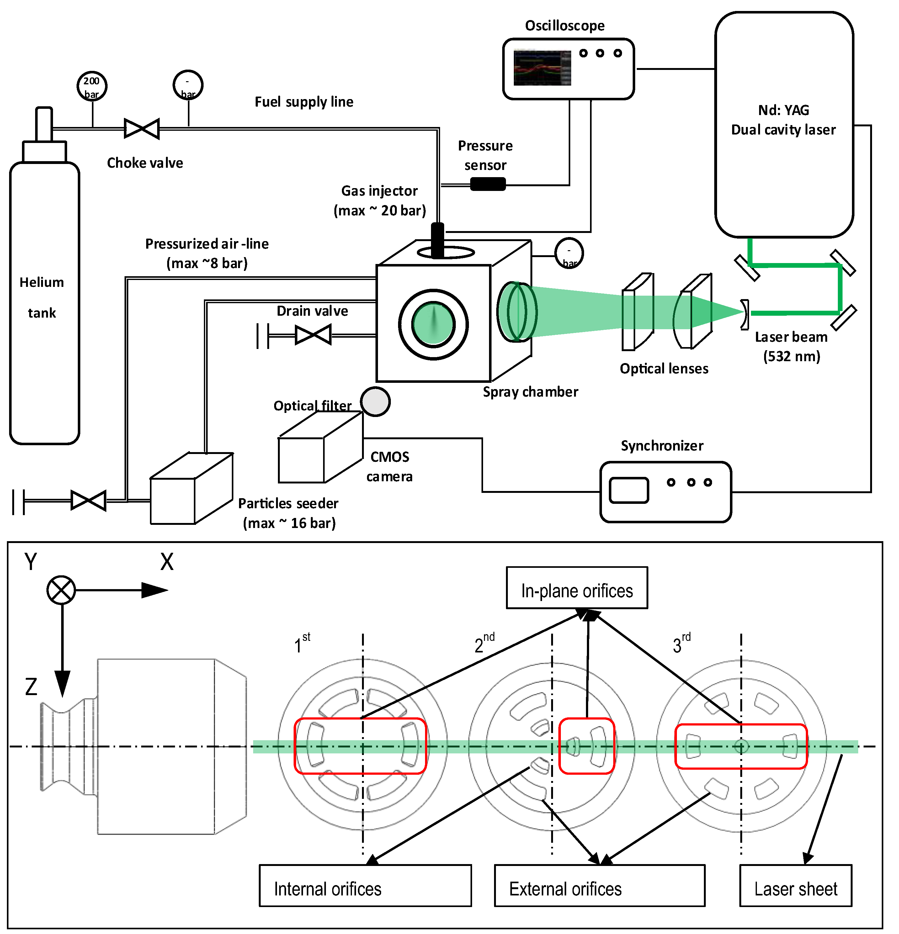
2. Experimental Setup

The schematization of the experimental setup and of three nozzle patterns are shown in Figure 1. A dual cavity Nd:YAG laser (Spectra Physics, Quanta Ray PIV-400, Milpitas, CA, USA) was used for the generation of the luminous background through the emission of two pulsed signals of light with a wavelength of 532 nm. The nominal energy of pulsed light was approximately of 60 mJ, having a duration of 6 ns and a time separation of 3 µs. Since it was not possible to know a priori the correct time delay between the two pulses, the above value was found by linearly increasing it from 1 to 15 µs during experiments at intermediate pressure ratio, i.e., PR10. The two laser pulses generated by the laser are then deviated by a series of mirrors and directed towards the CVC as shown in Figure 1. Before reaching the chamber the two signals pass through three cylindrical lenses; the first concave lens with a focal length of −50 mm and for the other two large lenses it was +500 mm. The two pulsed signals are thus converted onto sheets with a thickness of approximately 1 mm in correspondence of the injector axis. The air supply line reaches a maximum pressure of 8 bar and is connected to both CVC and particle seeder. The air input system in the chamber, as well as that for tracer particles, are designed to reduce their influence over the jet structure. Specifically, the air is supplied through a duct positioned on the upper wall away from the injector axis, while oil particles are conveyed through a perforated hollow toroidal tube located on the upper wall. Particular attention was paid to the calibration of the particle seeder to avoid two opposing conditions: lack or oversaturation of the tracer particles. This task was achieved by managing the inlet pressure of the particle seeder in relation to that of the pressure line. For the present study, the particle seeded was set to operate in order to produce tracers of 600 nm ± 200 nm. The resulting images of scattered light were recorded using an interline transfer camera (TSI 630090, Shoreview, MN, USA) with a resolution of 2352 × 1768 pixels and a 16-bit concentration per pixel. The helium was supplied from a tank at 200 bar and the gas injector mounted in the top wall of the chamber. The effective pressure of injection was set using a manual regulator and fluctuations monitored by a sensor. The pressure was observed to suffer a maximum reduction of less than 5% with reference to the nominal value, therefore influencing in a negligible way the flowrate characteristics. Optical access to the CVC was provided by four circular windows located on the side walls, each with an inner diameter of 130 mm. For the present study, two of these windows were obscured using laser beam stoppers or black screens. As for the three nozzle tip models (Figure 1, bottom), the geometric angle of divergence of the orifice paths from the injector axis was 15° for the first, 18° (external orifices)–12° (inner orifices) for the second and 20° for the third. The total area of the orifices on the nozzle tips is equal to 7.0, 4.3 and 4.0 mm2 for the first, second and third geometries, respectively.

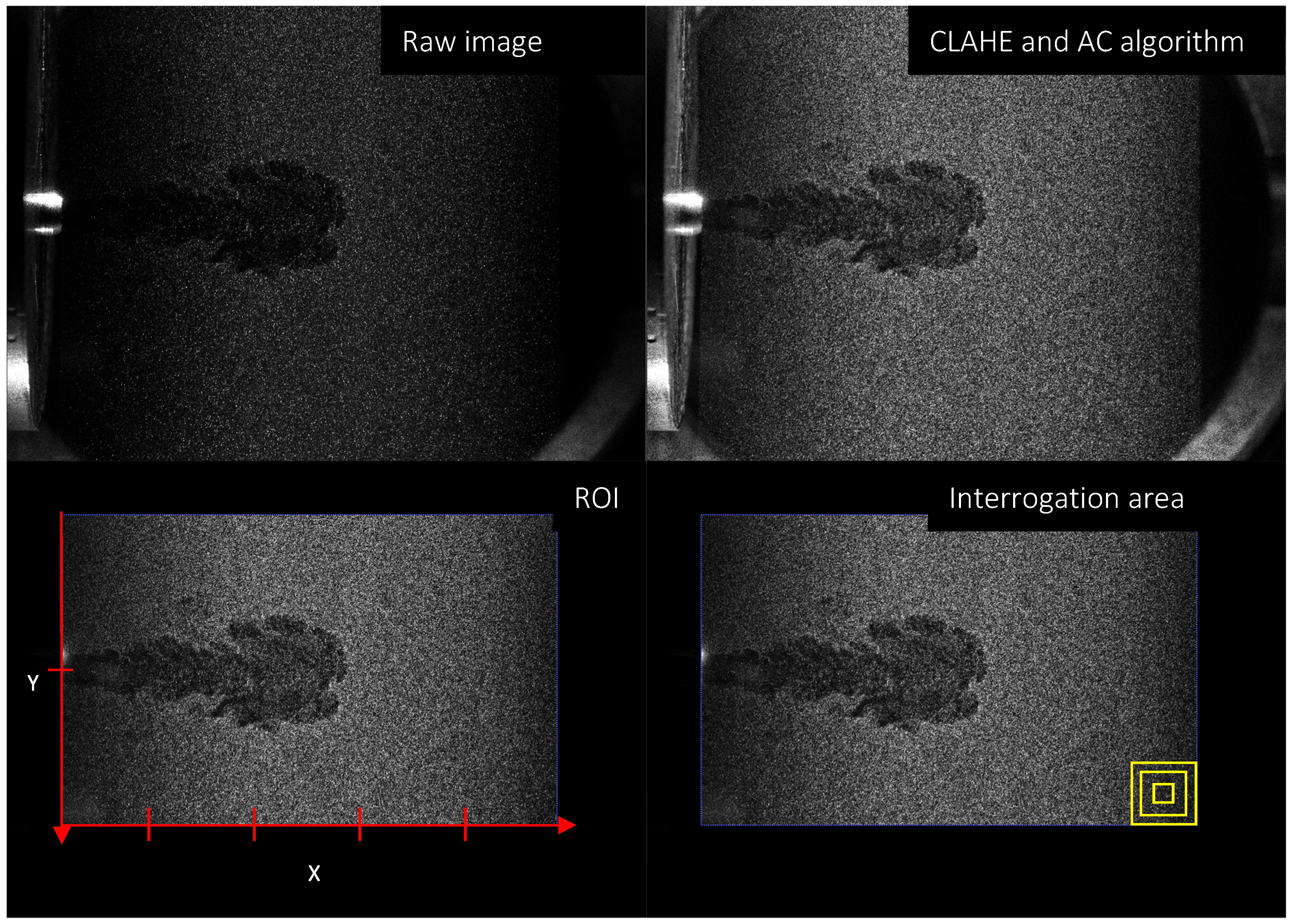
3. Software and Methodology

The cross-correlation algorithm was applied to evaluate the tracer particles displacement and the software used for this purpose was the Matlab R2022b (Natick, MA, USA) tool: PIVlab v2.61. Before proceeding with the algorithm, the scattered images were post-processed to improve their quality and to define the coordinate center reference system as shown in Figure 2. The jet object has been put in the foreground by using the contrast limited adaptive histogram equalization (CLAHE) and auto-contrast (AC) algorithms. The first is an image pre-processing technique that improves contrast in images. This algorithm elaborates several histograms, each corresponding to a distinct region of the raw image and uses them to redistribute the luminous values of the image [31]. Differently, the AC algorithm linearly stretches and offsets the image intensities. The next step involved the definition of the region of interest (ROI). This is the area within which the software performs the cross-correlation analysis. For the present work the ROI was set equal to 50 × 75 mm, and the x-y-center was positioned at injector tip as shown in Figure 2. The diameter of the nozzle tip was used to calibrate the spatial resolution of the PIV images, thus measuring the pixel/millimeters ratio. Next, it was necessary to choose the dimensions of the interrogation area (IA) whose size defines the resolution of the PIV analysis. It was decided to use a square-shaped IA with a multi-pass approach. This methodology causes the software to start performing the cross-correlation analysis by imposing an initial oversized interrogation area (defined by the user). This preliminary operation will turn a “rough” vectors distribution, then the software repeats the cross-correlation with a reduced size of the IA (normally it gets halved with reference to the initial value), returning a more detailed vector distribution, thus gradually increasing the accuracy of the PIV analysis. For the present study, a 3-step cross-correlation approach was used, and the starting size of the IA fixed equal to 64 × 64 pixels, then decreased to 32 × 32 and finally to 16 × 16 pixels (≈0.8 × 0.8 mm). A 25% overlap between neighboring cells has been applied for the correlation of the two consecutive frames.
For all operating conditions, two filters were applied to reduce the presence of spur vectors. First, a standard deviation filter was used to remove vectors whose magnitude exceeded the threshold defined by the following equation:
T r u e / F a l s e   V _ m e a n + n d e v . s t
where V_mean is the average velocity measured over the total spatial grid, n the user-imposed multiplier and dev.st the standard deviation. For the present study, n was set equal to 10. The second filter applied is a local median filter. In a 2-dimensional analysis, such as that considered for the present work, the filter considers neighbor values to calculate a moving average to limit the presence of local spikes. The window size has been set equal to 6 × 6 cells. Note that both filters discussed above were set to operate in a non-aggressive manner, due to the low number of spur vectors measured in raw vector grids.
Regarding edge detection, although it is necessary to measure jet penetration and plume angles, this information could not be directly extracted from the post-processed images. The high pixel density and local inhomogeneity typical of this type of analysis led the software to interpret the data as point-like, making impossible the identification of a coherent boundary between the jet and the background. For this reason, the jet edges were measured using a dedicated code built on Matlab R2022b by setting a threshold to separate the jet from the surroundings. This value was set equal to 20% of the maximum speed.
However, it is worth noting that the PIV provides an indirect measurement of flow velocity; therefore, this technique is subject to a certain degree of uncertainty, which can be estimated from Taylor series propagation and expressed by the equation:
U u u 2 = U X X 2 + U t t 2 + U M M 2
where u is the velocity at a point (x,y), calculated by measuring the displacement ∆x during time interval ∆t, and Uu represents the corresponding uncertainty. Then, the three variables refer to the uncertainty due to the displacement UX, laser pulse separation Ut and magnification UM contribute. The last two parameters depend on laser characteristics (normally Ut is around 1 ns, leading a negligible errors for most experiments) and correct calibration of the camera with respect to the optical window, that for the present study has been calibrated for adjusting the height of the CVC using spirit levels and monitoring the spatial resolution with respect to the injector tip size. Differently, the first variable depends on the error between real displacement and that measured. Since it is not possible to know a priori the true displacement, the uncertainty quantification is demanded to different theoretical models or by specific experiments in controlled environment [32]. Nevertheless, the accuracy of the PIV can be improved in many ways; among these, the use of multi-pass cross-correlation algorithm has been proven to reduce the error between measured and true displacement. Furthermore, the Stokes number (Stk) can be used to quantify a particle’s ability to follow the flow. It is defined as follows:
S t k = ρ p d p 2 U 18 μ L
where ρp is the seeded particle density (vegetable oil ≈ 900 kg/m3), d2p the diameter (≈600 nm), U the velocity, μ the dynamic viscosity (1.98 × 10⁻⁵ Pas) and L the characteristic length, which depends on orifice size. Regarding the speed, considered the condition with a ∆P of 19 bar (PCVC 1 bar–PINJ 20 bar), in proximity of the injector tip the flow can be assumed to be in choked conditions (See Equation (5)); then, the equation to calculate the velocity becomes
U = γ R T
where γ is the specific heat ratio of the gas (≈1.66 for helium), R the gas constant (2077 J/kgK) and T the temperature (300 K). The calculated speed is of approximately 1020 m/s. Since, at the early stages the jets emerging from the orifices are still separated, the characteristic length used in the Stk formula is set equal to the equivalent diameter of the single orifice. For example, for the first geometry, the characteristic length is 0.3 mm, and the calculated Stk is greater than 1, suggesting a slow particle response to flow acceleration, which justifies the presence of the weak correlation area. The situation rapidly changes downstream of the tip (5–15 mm depending on PR), where the maximum velocity recorded by the software decreases to 250–300 m/s and the individual jets merge into a single structure with an average diameter ranging from approximately 1.8 to 3.8 mm, depending on the nozzle geometry and operative condition. In particular, at PR20 in correspondence of the peak velocity, the Stokes number falls within a much lower range, from 0.07 to 0.09, indicating the particles’ ability to accurately follow the flow under subsonic conditions.

4. Results and Discussion

The experimental test campaign implied the use of helium as a hydrogen substitute. The operative conditions were chosen in order to gain an extensive understanding of jet propagating process (Table 1). With a pressure ratio over 3 (or 2 theoretically) it is expected to have choked flow and sonic velocity at the exit of the nozzle. The critical PR represents the threshold above which the flow reaches the sonic conditions and cannot increase speed despite a lower pressure downstream the circuit. The choked conditions at the nozzle tip are defined as follows:
P I N J P C V C = γ + 1 2 γ γ 1
where the ∗ indicates the minimum ratio to achieve the sonic conditions, while γ is the specific heat ratio (1.66 for He). Applying the above equation, the critical pressure ratio is approximately ≈2.0. This implies that almost all tested pressure ratios exceed this threshold. Specifically, downstream of the nozzle, where the PIV becomes capable of providing reliable results, the velocity magnitude varied from 100 to around of 300 m/s, thus remaining always under the sonic regime

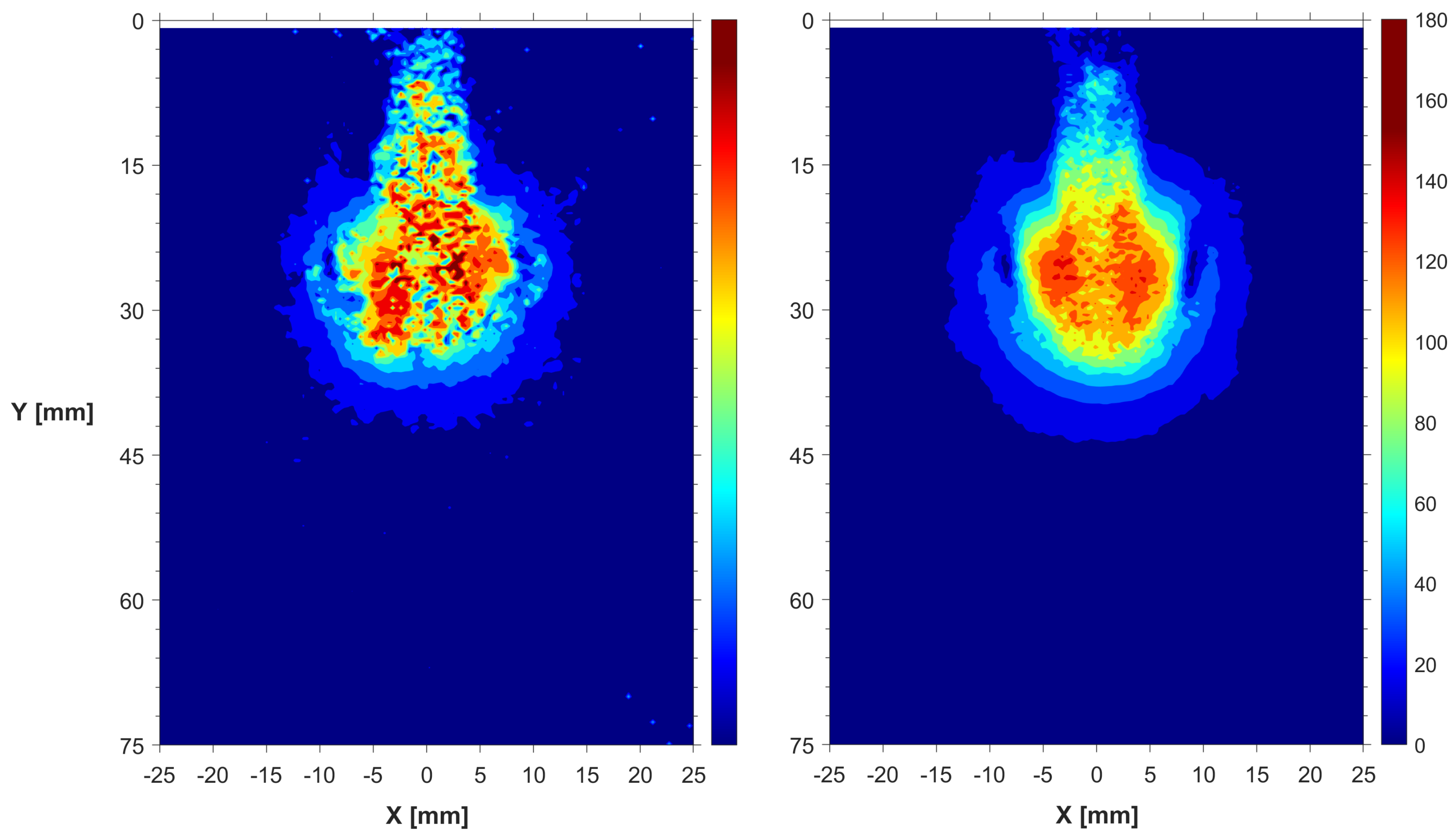
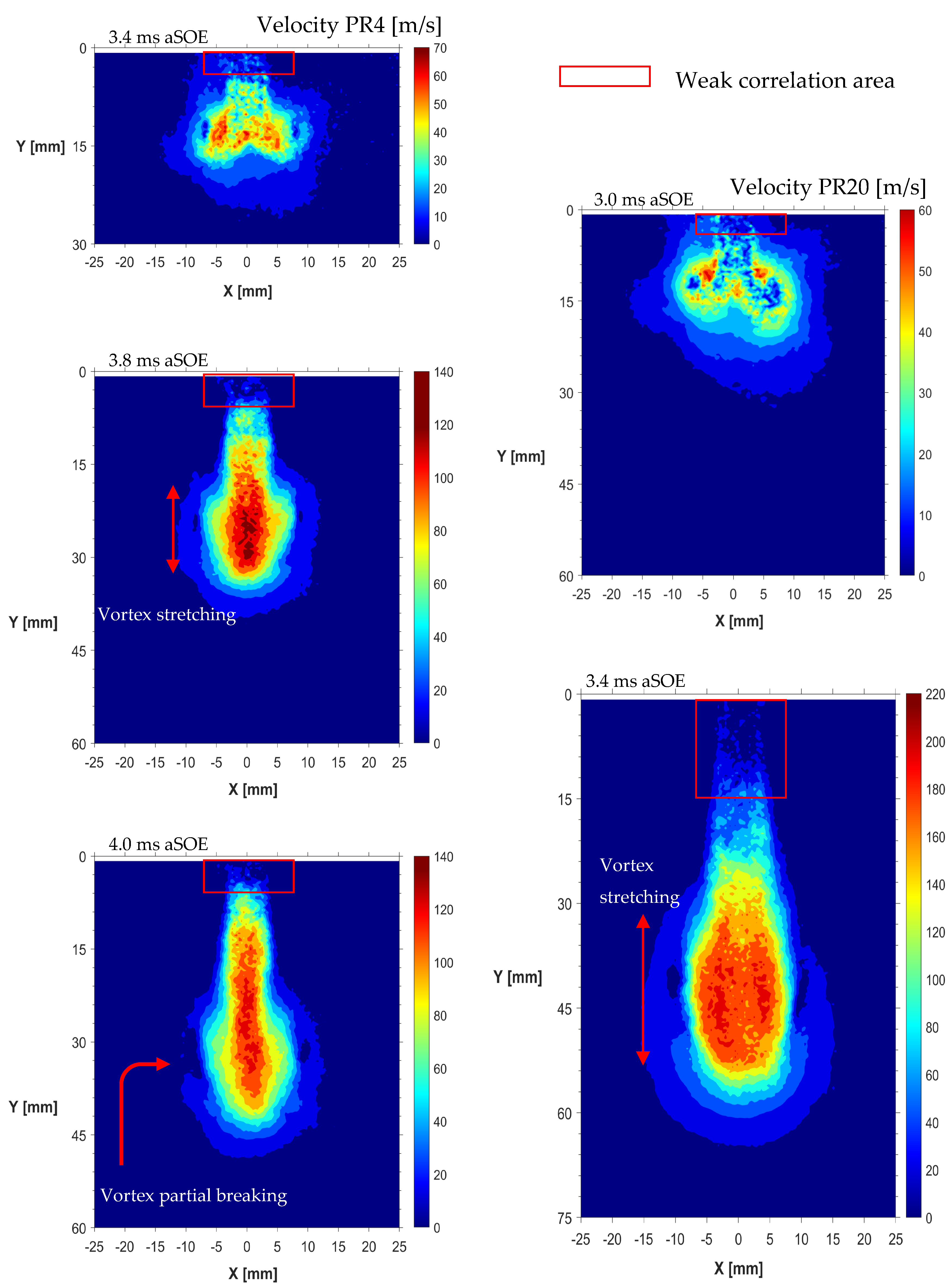
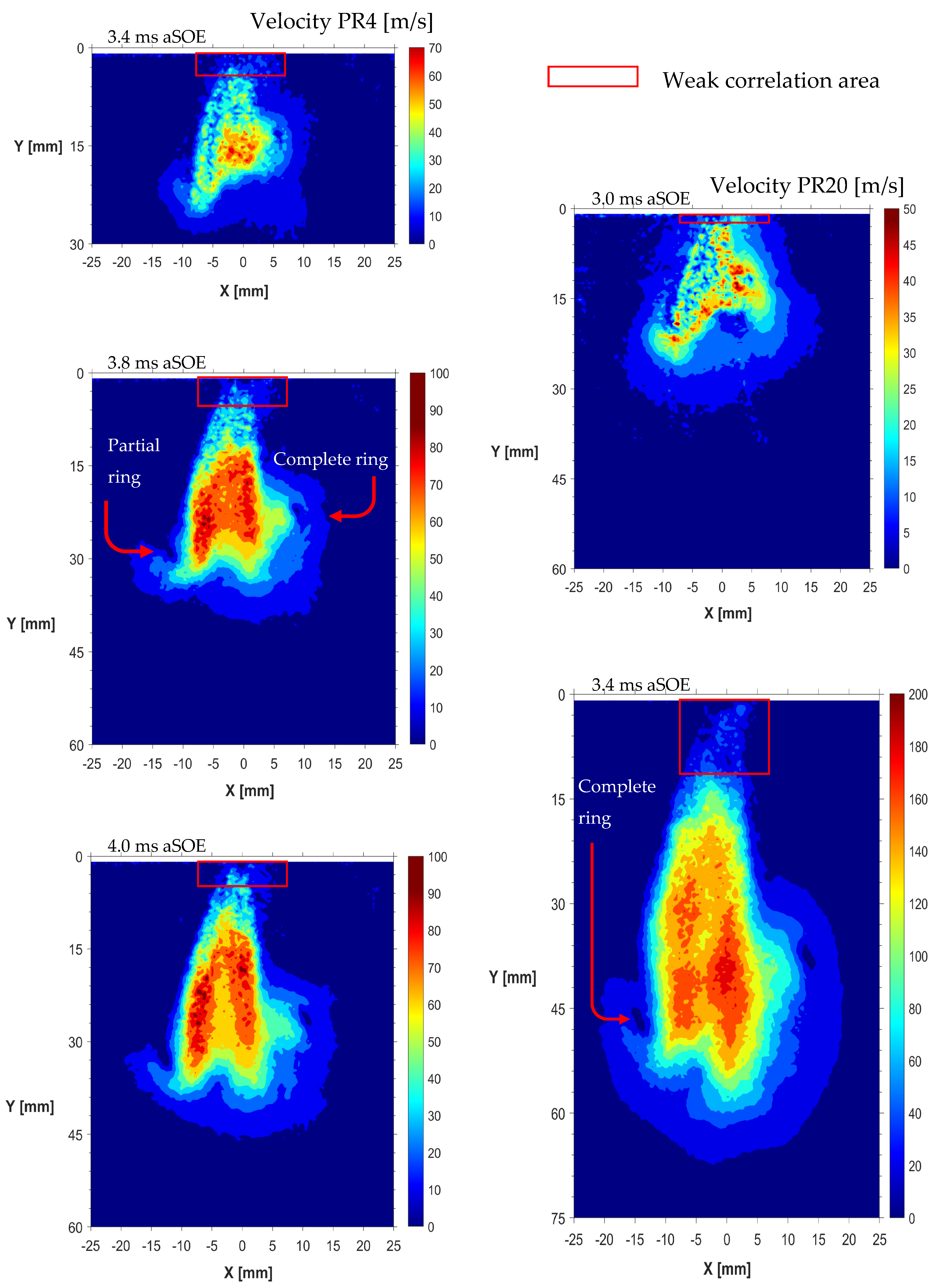
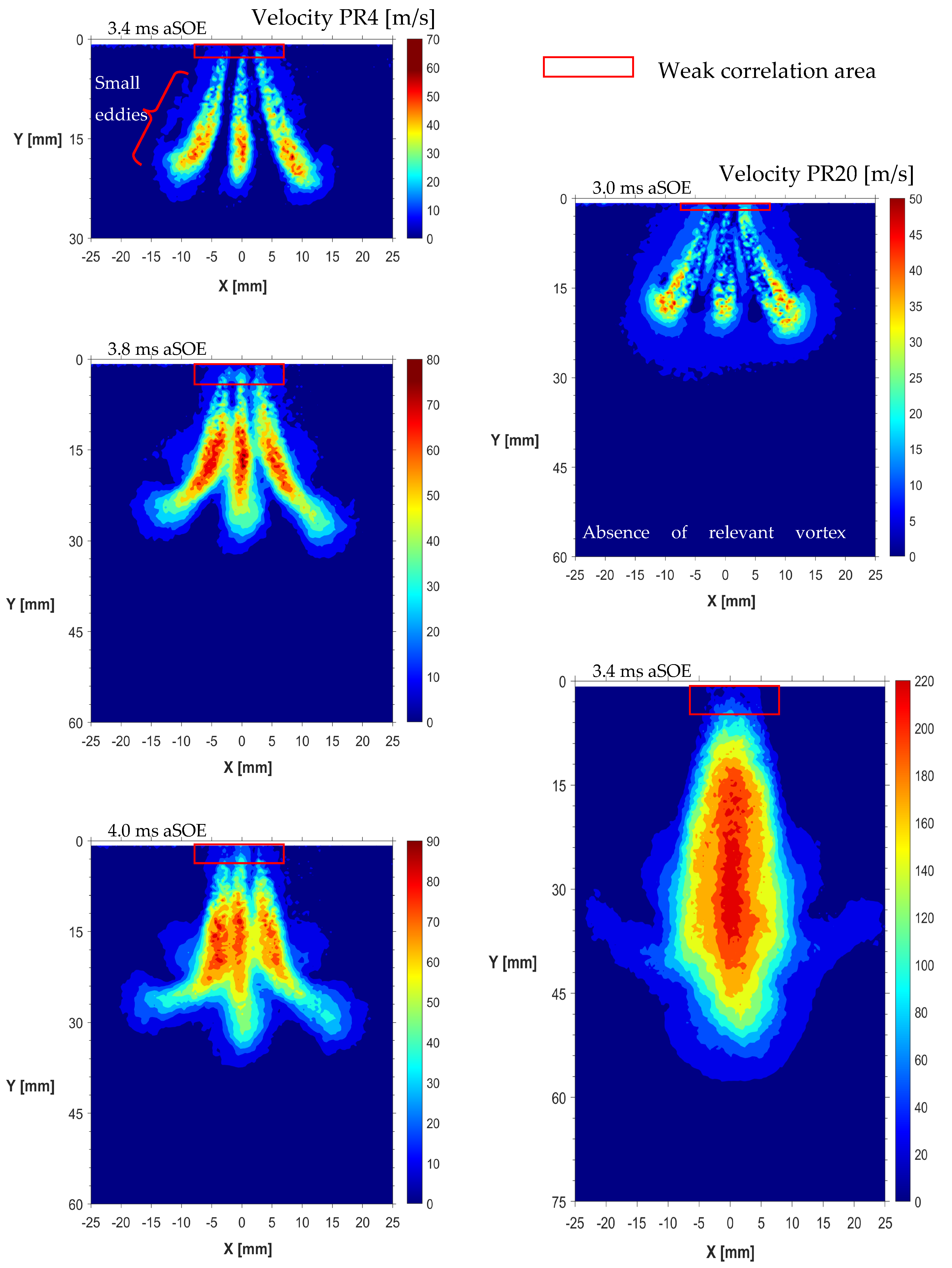
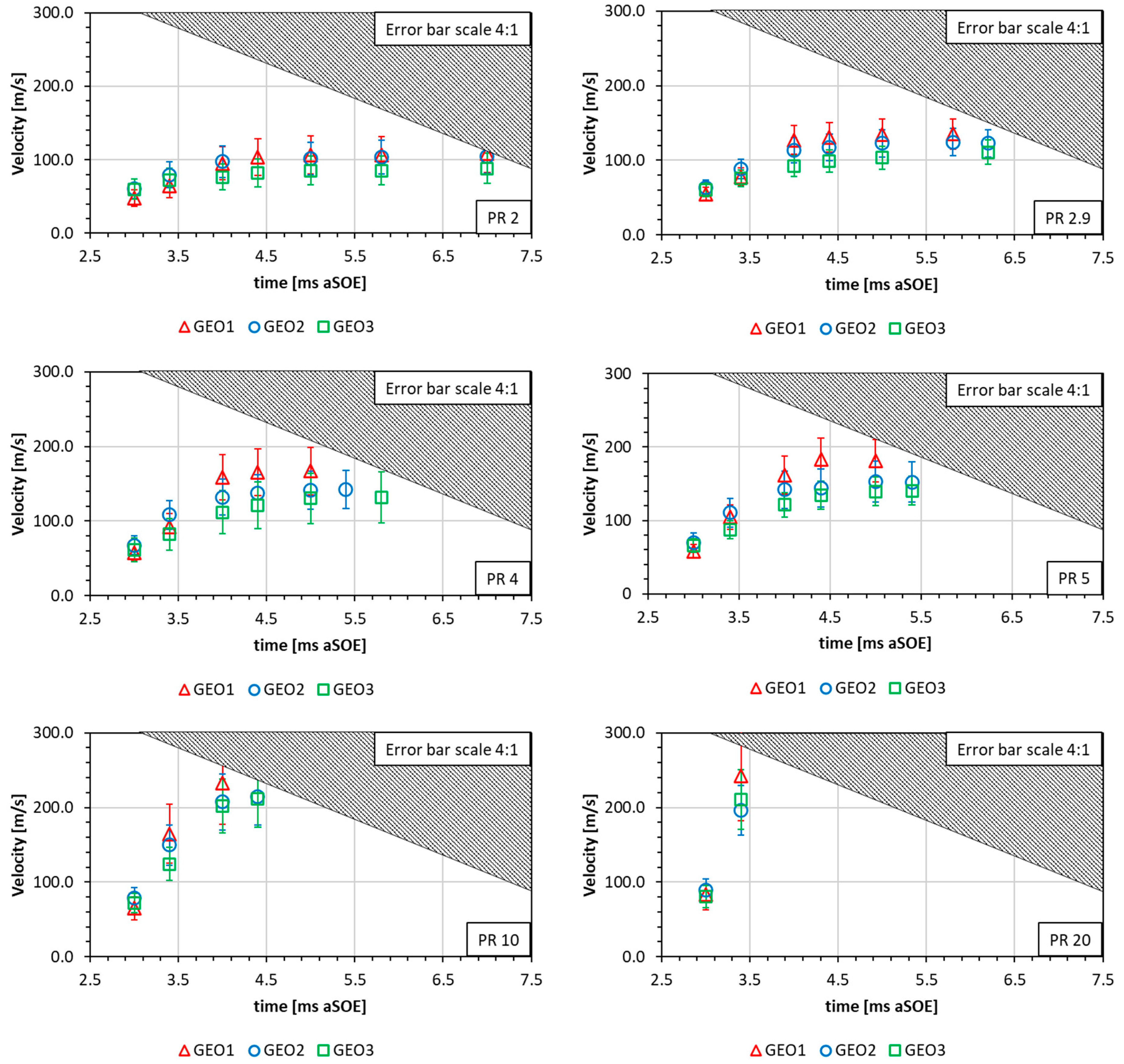
4.1. Velocity Magnitude

The results described and discussed in this section are based on an analysis performed on 20 pairs of frames recorded at different time-instants after the start of energizing (aSOE). It was experimentally observed that the first frame at which it was possible to see the jet coming out from the nozzle tip corresponded to the time instant at 2.7 ms aSOE. Specifically, the jet becomes appreciable at 3.0 ms aSOE, thus all the data discussed in this work range from this time instant onwards. Figure 3 compares the velocity distributions generated by a single pair of frames and that obtained by an ensemble of 20 pair of frames. As expected, the averaged image looks much more homogeneous and the velocity distribution well defined, highlighting the regions featuring different levels of velocity magnitude. Differently, the information coming from the single pair of frames appears fragmented with a more chaotic distribution of the sub-structures. For this reason, most of the data discussed in this and following section refer to the post-processed frames obtained by the average data. The drawback of using such type of data is related to the loss of part of the details in local vortex structures, as well as an overall reduction in the velocity magnitude (and vorticity intensity) caused by the random position of the peaks in the individual frame pairs, thus resulting in a lower value when “spatially” averaged.
For the sake of brevity, the next graphs will show the solely data recorded with PR 4 and 20, representative of the low- and high-pressure ratio conditions. Figure 4 illustrates the velocity distribution generated by the first geometry at high and low PR conditions, highlighting the differences in terms of jet extension, as well as the phenomena addressed to the formation of vortex structures. Specifically, two lateral vortices (recognizable by the presence of a quasi-static area surrounded by non-zero velocity regions) were noticeable since the very early stage of the jet development for both ratios. At PR4, as the jet extends these structures start stretching trying to keep pace with the jet head region, thus contributing to the entrainment of air from the rear area. In the advanced stages, these structures were noted to become unable to match the jet extension, losing their capacity to further penetrate along the jet axis, thus collapsing. These large vortexes improve their capacity to keep up with the jet as the pressure ratio increases. In this condition, the jet rapidly reaches the border of the ROI, i.e., ≈3.6 ms at PR20. In a 3D perspective, these rings can be assumed to generate a toroidal corona surrounding the jet, the main contributor to the air dragging from the rear area of the jet. However, the mixing efficiency was noted to be mainly demanded by these structures since the achievement of the steady state conditions; then they were replaced by many small eddies positioned downstream the nozzle tip. Figure 5 shows the velocity distribution of the jet generated by the second geometry. At PR4 condition, both jets remain recognizable for the entire duration of the sequence recorded. The interaction with surrounding air leads to the formation of two vortexes. The one on the inner side appeared more stable, with a well-defined center, contributing to the air dragging from the rear area. Differently, the one on the outer side the vortex lasted for a short period before collapsing, i.e., ≈3.4–3.8 ms. The presence of a low-speed region between the two jets was noted to form before the achievement of the steady state conditions. This area can be addressed to the presence of air in between the two jets, resulting in a local speed of around 45–50 m/s, while surrounded by the tail of the two jets at 90–100 m/s. At PR 20 condition, the overall increase in momentum of the jets makes them able to create more stable vortexes. In addition, opposite the low-ratio condition, the in-plane jet becomes predominant for extension, with the outer jet that rapidly fills the low-speed area, reducing the radial propagation of the entire structure.
The higher orientation of the outer orifices of the third geometry, as well as the increased distance between these and the central orifice, make it possible to clearly visualize the three jets cross sectioned by the laser sheet (Figure 6). Due to the small size of nozzle orifices, it was not possible to recognize any relevant vortex structure, regardless of the PR condition. Further, it was noted that the radial propagation grows until the head of the lateral jets deviates towards external regions. At this stage, the velocity magnitude of the lateral jets rapidly decreases to less than half of the maximum value. In this condition, the fresh charge of helium coming from the rear area sweep away the lateral jets head. Among all the injector tips investigated, the third geometry produced in the shortest jet, and the short distance between external orifices did not allow for the presence of low-speed regions, thus demanding the mixing efficiency to the small eddies. Further, the velocity magnitude measured is the lowest among that observed, with an overall gap about of 15–20% compared to the first geometry and 5–10% to the second.
In Figure 7 the maximum velocity values for each case are illustrated. Those shown in the graphs are the values calculated by the 20 peaks measured for each individual pair of frames, while the dashed area represents the ROI border. The largest size of first geometry nozzle cap orifices always ensured the achievement of the highest values of velocity magnitude, regardless of the PR condition, which ranged from 108 to 242 m/s. In particular, at early stages the second and third geometries were observed to be slightly faster than the first nozzle pattern, with a gap ranging from 10 to 20%. In this phase, rather than orientation, the size of the orifices on the nozzle tip plays a key role in restricting the jet, giving it a better ability to penetrate through the air. This trend is reversed between 3.4 and 4.0 ms aSOE, when the first geometry becomes faster than other configurations. The gap between the three configurations rises as the PR increases, with the first nozzle leading to a difference in a few percentages at low PR, to slightly more than 20% of PR10 and PR20 cases.
Regarding the range of the reported average data, it was observed that velocity peaks exhibited a higher standard deviation in the moments subsequent to the injection trigger, with values ranging between 6 and 11%. This is attributed to the influence of the low-correlation area. As the jet extended, this value rapidly decreased, reaching values between 3 and 6%, with an improved reproducibility of the velocity peaks noted at higher PR values. In particular, the third geometry was found to be the most stable with standard deviation ranging from 3 and 5% under most operative conditions.
However, it is worth noting that the values determined in Figure 7 refer to the velocity calculated in the jet core, rather than near the nozzle tip, since in this area a sufficient number of seed particles are not yet trapped to follow the jet flow. A further set of 20 pairs of frames was recorded at 8.0 ms aSOE for each ratio examined, when the jet was in steady state conditions. The recorded maximum speed values are presented in Table 2.
The data listed in Table 2 have been used to calculate the Reynolds number (Re). The latter is a dimensionless quantity defined as the ratio between inertial and viscous forces. The Reynolds number is used to characterize flow regime, and it is calculated as follows:
R e = ρ U D μ
where ρ is the gas density, thus ≈ 0.85, 1.71 and 3.43 kg/m3 for helium at 5, 10 and 20 bar, respectively (at 300 K). U is the speed of the jet, D the characteristic length and μ the dynamic viscosity (1.98 × 10⁻⁵ Pas at 300 K). As far as the speed and characteristic length, it was noted that under steady state conditions the areas characterized by the highest values of velocity (the same presented in Table 2) were always located downstream of the weak correlation area, 5–15 mm far from the injector, depending on the pressure ratio. At this distance, the jet width is rather narrow and by setting a threshold equal to 80% of the maximum recorded velocity, to assume the presence of only helium [33], the jet core size was measured. The calculated Re number values are listed in Table 3.
All the operating conditions examined fall within the turbulent flow regime. The first geometry was the most stable, returning a jet diameter of approximately 3.5–3.8 mm at peak velocity. In contrast, the second and third geometries revealed a higher degree of variation in this parameter. More specifically, the second geometry returned to a diameter between 2.0 and 3.2 mm, with maximum value measured at intermediate PR conditions. The third geometry, on the other hand, showed the lowest diameter values, i.e., from 1.8 to 2.2 mm, except in the case of the most severe injection pressure. At PR 20 the three jets merged in a single structure, leading to an increase in the overall jet width to 5.4 mm near the peak velocity.

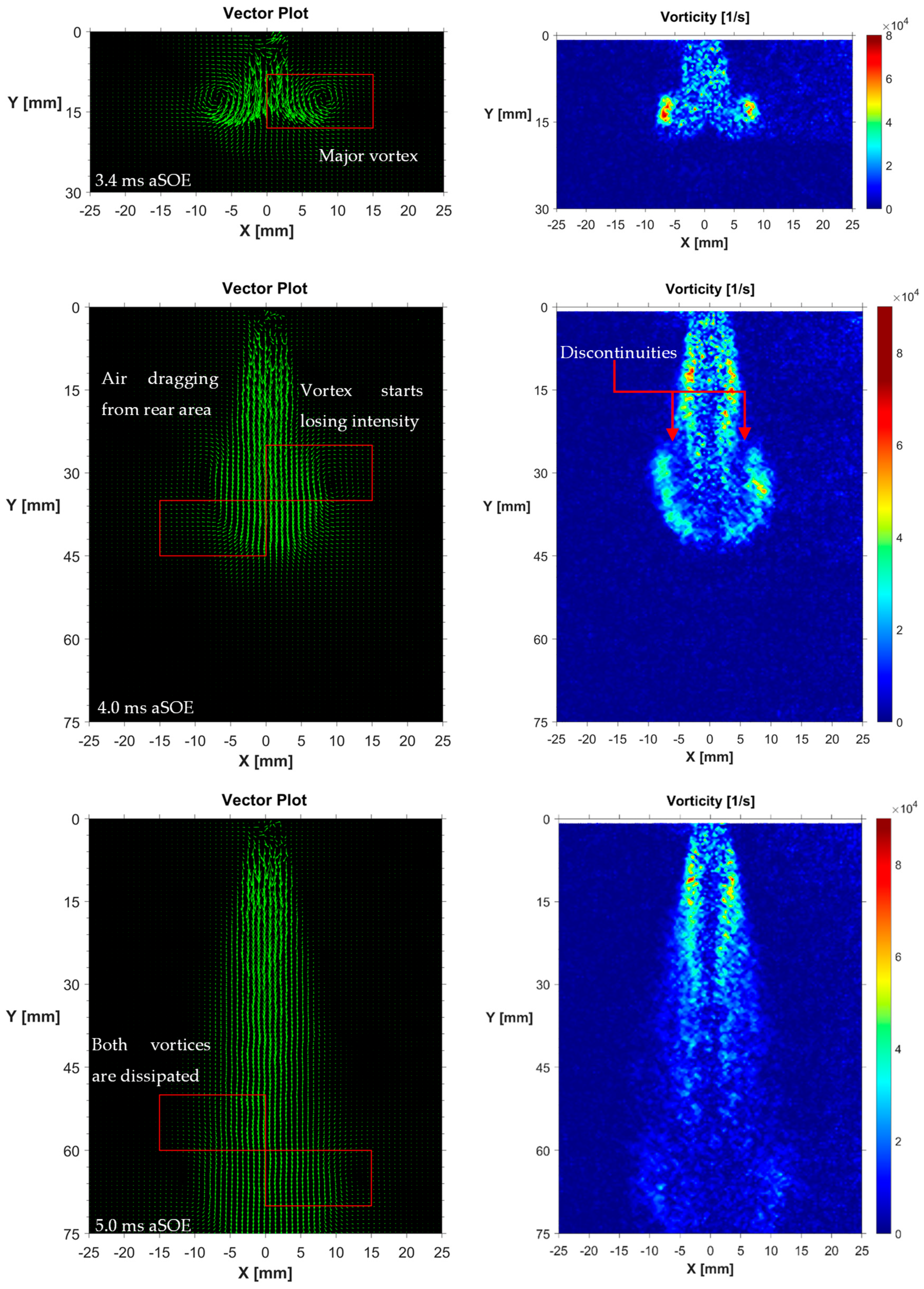
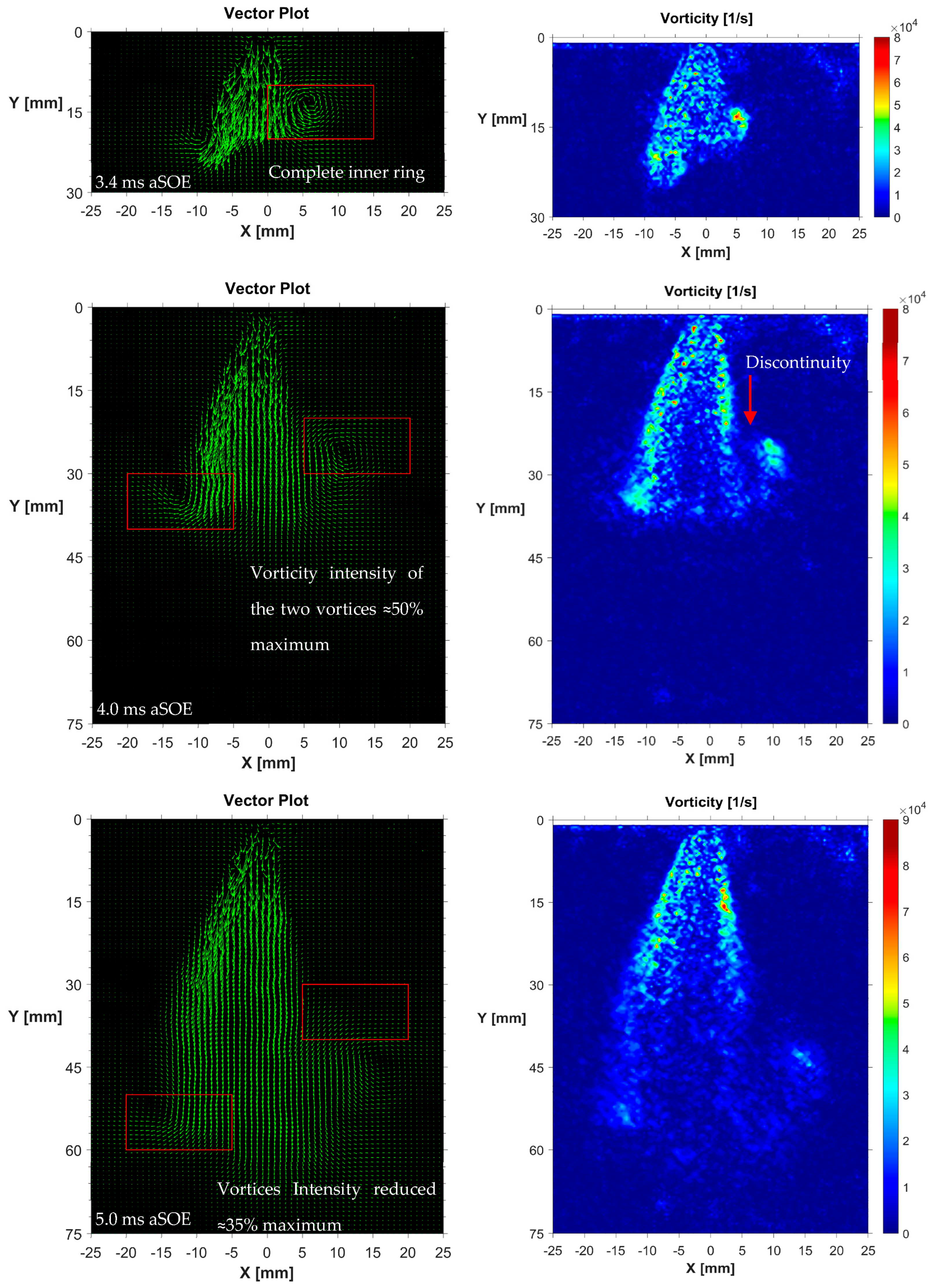
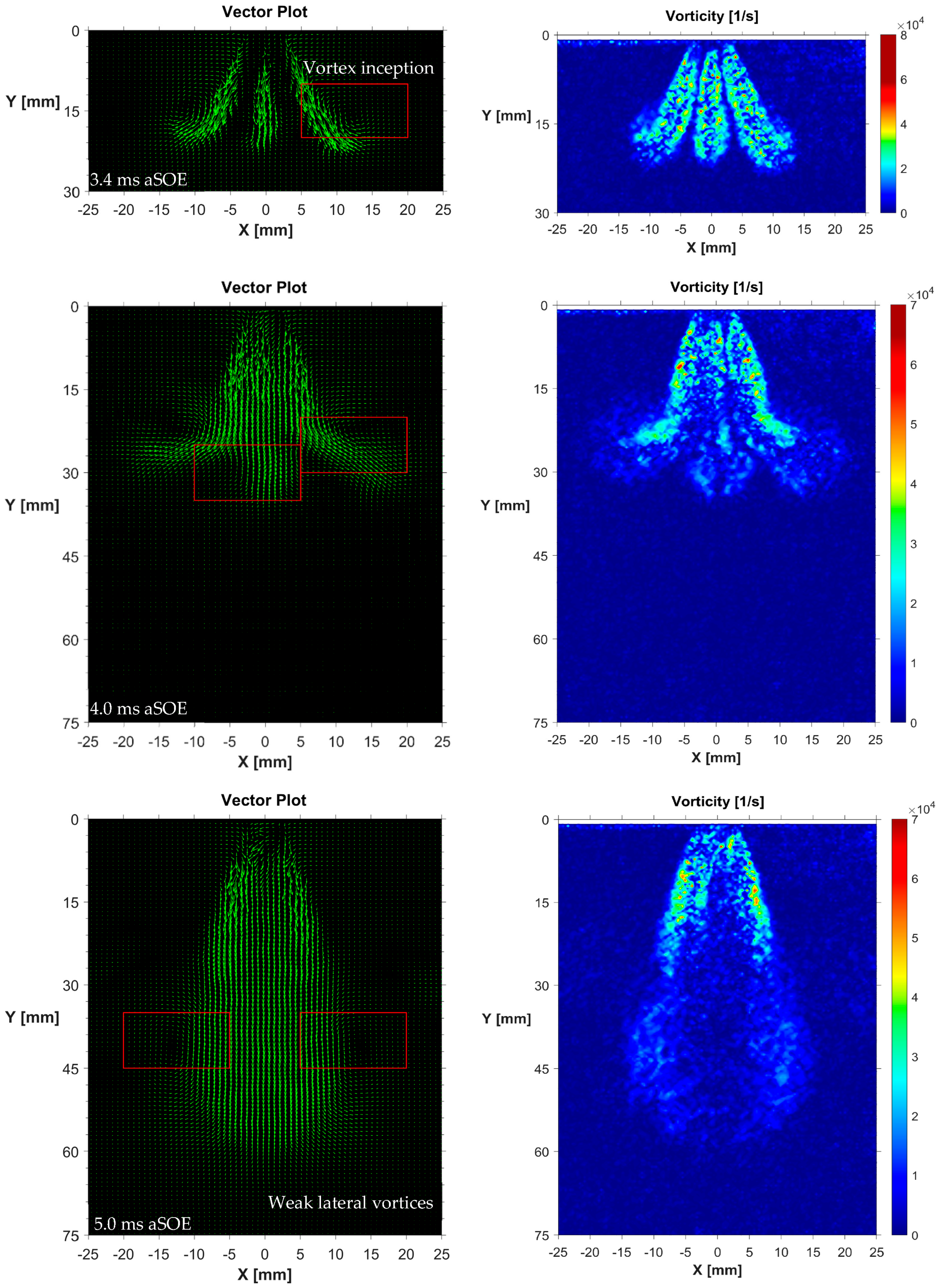
4.2. Vorticity Intensity
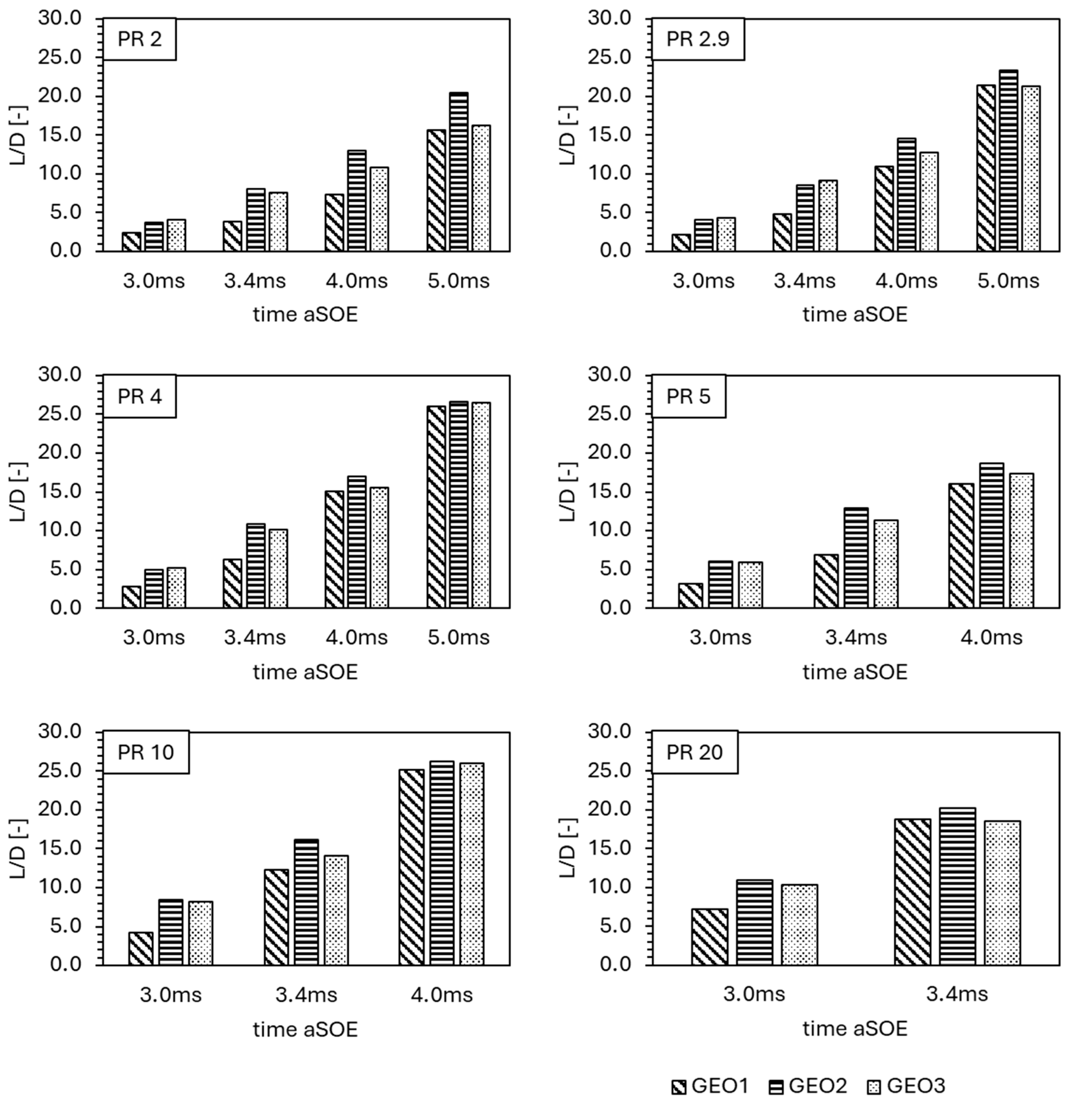
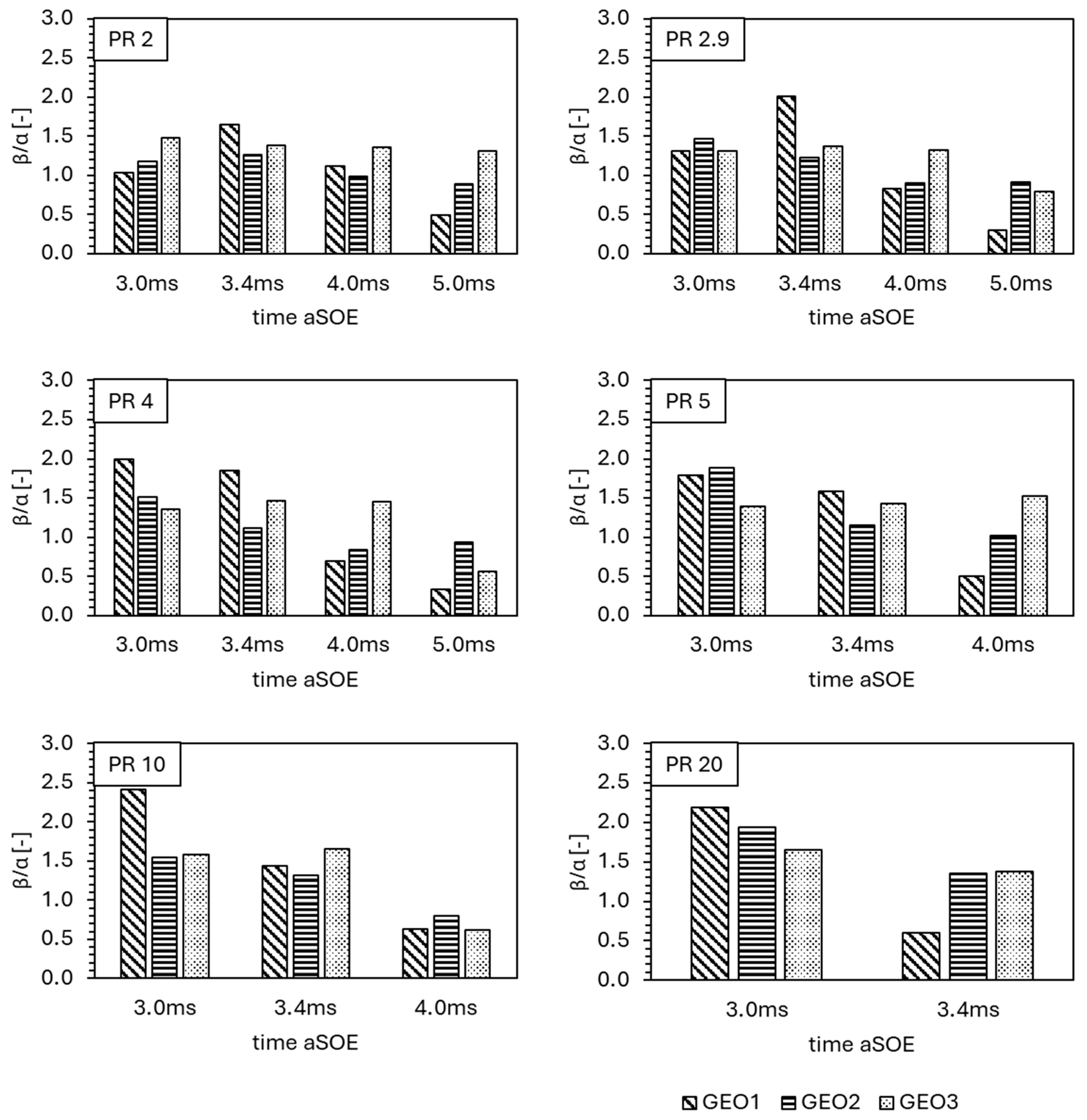
Considering any point traveling along with the flow under investigation, the vorticity intensity is defined as the pseudovector field which describes the local spinning motion of such point. Mathematically, it can be expressed by the equation,
ω v
where ∇ is the nabla operator and v the flow velocity. In a two-dimensional analysis, Equation (7) becomes
ω = v y x v x y e z
where ez is the versor along the zeta-axis. During the post-processing of the images the vector field was observed not to change in a significant way, in terms of development pattern, with the pressure ratio. These results, coupled with the large amount of data recorded, led to the decision to illustrate in this section solely the images related to the operative condition at PR4. Specifically, graphs shown in Figure 8, Figure 9 and Figure 10 were drawn from an ensemble of 20 pairs of frames. Figure 8 shows the vector plots and corresponding vorticity distributions produced using the first nozzle tip geometry. At early stages, two vortexes were visualized on the head section of the jet and the instantaneous center of these rings corresponds to the position of the vorticity peaks. Here, the vorticity intensity reaches values of approximately 85,000 1/s. In a 3D perspective, these two vortices can be assumed to be connected by a toroidal ring surrounding the jet head. The acceleration caused by the continuous supply of helium causes the region downstream the nozzle tip to be characterized by increased vorticity during the entire duration of the injection. This region was noted to extend as pressure ratio increased, from just over 20 mm to almost the entire extent of the jet (≈70 mm). After 4.0 ms, two discontinuities separating the steady state region from the head region of the jet were visualized. In these regions the air is dragged inside the jet with an oblique direction that deviates the helium towards the center. This phenomenon leads to the flow “disconnection” between the head section and the rear area. Without the supply of helium, the two vortices positioned on the head therefore become unable to sustain the rotative motion, rapidly dissipating their vorticity intensity. At 5.0 ms aSOE, the only relevant regions for the interaction between gas–air remain that close to the nozzle tip. There, the constant supply of helium contributes to the establishment of small eddies which size is lower than the resolution applied for the present study (≈0.8 × 0.8 mm), thus impossible to be individually recognized. It is worth noting that the first geometry is the least-oriented one and that in agreement with jet models present in the literature, i.e., [34,35], it clearly shows the presence of two vortices surrounding the jet head from the early stages. These vortices trigger air entrainment from the side regions and gradually lose intensity as the jet propagates.
Figure 9 provides a closer look at the jet produced for the second geometry. Since early stages, the two jets coming from the inner and external orifices work differently in terms of interaction with air. The external orifice, which is the most oriented one (18°), generates an oblique jet able to keep momentum better than inner component, resulting in a greater extension. In contrast, on the inner side the vector plot shows the presence of a complete vortex. At 4.0 ms aSOE, the inner ring starts losing intensity for similar reasons to that seen for the first geometry. The anticlockwise motion triggered by the vortex brings to the opening of a discontinuity in the vorticity distribution. This lack of fresh charge from the rear area contributes to a significant loss in intensity of the inner ring, whose value is now around 40,000 1/s. Differently, the outer jet start slowing its radial spreading. This phenomenon can be attributed to two causes: the increase in CVC pressure that implies the onset of a “confinement” action on the jet and the presence of the low-speed area between the jets produced by the external and inner orifices. To pursue this hypothesis, the plume angle of the jet was observed to reduce as the air backpressures increased. At 5.0 ms aSOE, both jets are surrounded by multiple peaks, with the inner side showing slightly higher values of vorticity intensity. Similarly to the first geometry, rather than significant vortex structures, there are small eddies to drive the mixing efficiency of the investigated geometry when the jet is fully developed. In this phase, the maximum intensity value is around 85,000 1/s. The various stages of flow field concerning the third geometry are illustrated in Figure 10. In the first phase, subsequent to the start of the injection, the three in-plane jets are clearly visualizable showing similar peak values of vorticity intensity, i.e., ≈75,000 1/s. A similar extension of the central jet is possible due to the shorter path that helium has to follow when passing through the central orifice, thus compensating its smaller size compared to that of the external orifices. Unlike geometries discussed so far, no significant vortexes were noted at 3.4 ms aSOE. In particular, the external jets contribute to the formation of two partial rings, whose intensity is quite reduced compared to the small eddies occurring over the jet edges. The reasons for the absence of relevant vortex structures can be addressed to the relatively small size of the orifices and their orientation which led to the generation of narrow and separate jets, thus able to keep the momentum without losing energy to the surrounding air. At 4.0 ms aSOE, the external jets deviate towards lateral regions, losing their capacity to further penetrate along injector axis. The helium coming from the nozzle tip reaches these areas with a higher velocity, which the vertical component dominates (vy), thus unable to follow the deviation and leading to the breakup of these structures. After 5.0 ms, because of the constant supply of helium from within the main flow, the two side structures are no longer visible, leaving a single larger jet that is characterized by a higher plume angle compared to the first geometry jet, but with a lower velocity magnitude. In any case, it clearly appears that regardless of the nozzle pattern the large vortex structures move with a speed that is somewhat smaller than that of the jet head, highlighting a tendency of these rings to “slip” on jet borders before collapsing. These findings agree with those discussed in [36].
It should be noted that as the angular spacing between individual jets increases, they become unable to merge into a single coherent structure. This reduces their ability to interact with the surrounding air, thereby promoting vortex formation. Among the few studies available, these findings are in line with those reported in [37]. Figure 11 shows the absolute peaks values of the vorticity intensity measured by the three geometry nozzles for the various PRs examined. Specifically, first and second geometries alternate randomly, while third geometry showed an overall lower value of vorticity intensity. Further, unlike velocity, which increases linearly till the achievement of the ROI border, the peaks in vorticity were observed to stabilize at almost constant values after 3.5 ms aSOE, regardless of the nozzle tip. Given the definition of the vorticity intensity, it is therefore possible to suppose that as the average velocity of the jet increases, the instantaneous radius of the vortex structure is reduced. This hypothesis is in line with the observed tendency of the major rotational structures to extinguish as the jet develops. Other factors contributing to that phenomenon could be related to the longer time for the merged jet to form (from individual or a ring-shaped jet) and reach its stationary velocity, than it takes for the vortex structure at the upper part of the jet to form.
However, looking at peak values alone, another difference to velocity is that, considered a specific geometry at a fixed time instant, it does not undergo the same change in magnitude by increasing the PR. Just by way of example, at PR2 and 3.4 ms aSOE, the average velocity recorded by all geometries was about 80 m/s, then increased up to 200–250 m/s at PR20. Differently, applying the same approach to vorticity intensity, this value increases from 120,000–140,000 to 200,000–235,000 1/s. Unlike the velocity, the variability of the vorticity is significantly higher, with standard deviation values ranging from 8% to 25%. The highest variability was observed at 3.0 ms aSOE under low PR conditions, with the first and second geometries being less stable than the third. However, as the PR increased, a reversal in this trend was observed, with the third geometry becoming less stable than the other two. Hence, the ratio between the low and high PR conditions reduced from almost 3.0 in velocity to 1.8 in vorticity. The values recorded at 8.0 ms aSOE are listed in Table 4. The vorticity intensity now relies on more comparable values, where the highest gap was measured between first and third geometry at PR5, thus equal to slightly less than 10%.

5. Jet Morphology

Another aspect examined in this work is the morphology of the jet/s, thus its penetration and the plume angle. Both parameters were measured through the use of a code built on Matlab used to detect the edge of the jet. The working principle of the code is based on the velocity threshold defined by the user to return the coordinates of the borders all around the jet perimeter. More in detail, considering the generic operative condition, the threshold value was set equal to the 20% of the mean value of the peak velocities of all 20 frame pairs, thus using a less severe approach compared to that used for measuring the size of the jet core for recalculation. The jet penetration values were normalized with respect to the diameter of the nozzle orifices. In particular, considering the tendency of the individual jets to merge into a single structure from early stages after injection, an equivalent diameter was hypothesized based on the total orifice area. Accordingly, the measured penetration values were normalized using diameters of 3.00 mm, 2.35 mm and 2.25 mm for the first, second and third geometries, respectively. The resulting normalized values are shown in the histograms in Figure 12. The graphs below confirm that the first geometry exhibits the slowest jet penetration in the early stages, showing a significant gap compared to the other two configurations. This phenomenon can be attributed to the near-instantaneous collimation of the individual jets into a single coherent structure, which initially reduces the axial velocity. However, this structure becomes more effective in sustaining penetration in the mid-to-long term. In detail, the jet produced by the first accelerates faster than the other two configurations, with an increasing gap ranging from 15% to 30% with the other two geometries before achieving the edge ROI. The second and third nozzle tips are more directly comparable, having similar equivalent diameters but different nozzle layouts (see Figure 1, bottom). In particular, the reduced spacing between the inner and outer orifices in the second geometry promotes more effective jet penetration, especially under low pressure ratio (PR) conditions. The increased orifice size and reduced inclination in the second geometry offer an initial advantage in jet penetration, which reduces as PR increases. Ultimately, L/D values tend to converge across the two configurations examined, emphasizing the influence of orifice angle over shape, and suggesting that orifice spacing affects jet extension primarily during early injection stages. Noticeable is the variability that kept always showing in the reduced values, ranging from 1% to 5%, thus suggesting good repeatability for the measurement of the jet extension.
Regarding the plume angle, it is more appropriate to refer to half of the plume angle for this study. In fact, considering the three nozzle tips analyzed, the second geometry is the only one that does not provide a symmetrical view of the jet structure. It was therefore decided to measure only half of the above parameter, β. This parameter β was then normalized by the angle α, defined as the inclination of the external orifice channels relative to the injector axis (15°, 18° and 20° for first, second and third nozzle). The resulting ratio, β/α, provides a measure of how effectively a given geometry preserves or modifies the original geometrical dispersion angle. Figure 13 illustrates the histograms of the calculated values for all the configurations investigated. The large total surface area of the first geometry initially results in a high degree of jet dispersion, reaching up to twice the geometric angle. The subsequent collimation of the jets in a single structure drastically reduces this value, with the β/α ratio always ending below unity before the jet exits the ROI. In contrast, the second and third nozzle tips maintain a wider jet spread throughout the entire injection process. Specifically, the second geometry exhibits a linear decrease in the β/α ratio, while the third maintains an almost constant ratio until the collapse of the lateral wings (see Figure 10), which causes a sudden drop in the parameter. Noticeably, despite the higher geometric angle of the third nozzle pattern, it produces a jet that reaches the edge of the ROI with a smaller spread compared to the second tip. This difference can be attributed to the reduced size of the external orifice. Specifically, considering only the second and third external orifices (see Figure 1, bottom), there is an individual difference of approximately 64%, in terms of area (2nd > 3rd).

6. Conclusions

In this paper the particle image velocimetry (PIV) technique has been used to analyze the velocity and vorticity characteristics of helium jets delivered by a light-duty gas injector. Three complex geometry nozzles were used to thoroughly examine the effect of orifices size/orientation on velocity magnitude, vorticity and main jet morphological parameters. The constant volume chamber was seeded with vegetable oil droplets to make it possible to track the motion induced by the helium jet to the surrounding air. The image post-processing procedure made it possible to analyze readable images capable of providing global and detailed information on jet morphology and complex flow phenomena, such as the presence and distribution of vortex rings. The main results of the present investigation are listed below:
  • The results on vorticity intensity highlight the role of major vortex structures in early and middle stages after injection in promoting mixing phenomena. Then, these structures rapidly collapse, regardless of the nozzle pattern and PR condition, leaving room to the rise in number of small eddies. In particular, these micro-structures were observed to form downstream to the nozzle tip and extend for relatively short distance at low PRs (5–15 mm) and shifted along the injector axis (15–70 mm) at high PRs conditions.
  • Once the PR condition was established, the velocity magnitude was observed to increase almost linearly with time across all configurations examined. In contrast, after 3.5–4.0 ms aSOE, vorticity intensity kept an almost constant trend for each case considered. These results are in line with the absence of large vortex structures observed during jet development and the parallel increase in the number of small vortices.
  • The use of nozzle patterns with low orientation orifice paths, like first geometry, leads to the production of jets capable of keeping momentum, thus fastening the resulting jet at expense of a limited radial propagation, i.e., β/α < 1 at 8.0 ms aSOE. Specifically, the first configuration recorded the highest values of velocity peaks, i.e., from 105 to 309 m/s at 8.0 ms aSOE, regardless of the PR condition examined.
  • Second and third geometries, both featuring more complex multi-orifice nozzle patterns and a higher degree of orientation of the orifice paths, resulted in an improved radial propagation of the jet, i.e., β/α ranging from 0.5 to 1.5 before achieving the ROI border. On the other hand, the greater area of the jet impacting with the air involved a reduction in jet penetration along the injector axis. Specifically, the gap in velocity was measured to be around of 10–20% compared to first geometry during injection process.
The above results could become of paramount importance for the design of injection strategies, i.e., injection duration and interactions with the piston or cylinder walls, to improve the mixing efficiency depending on the application. Experiments consist of a valuable dataset to support 3D-CFD codes.

Author Contributions

Conceptualization, M.A. and S.S.M.; methodology, G.C.; software, G.C.; validation, G.C.; formal analysis, G.C.; investigation, G.C.; resources, S.S.M. and A.I.; data curation, G.C.; writing—original draft preparation, G.C.; writing—review and editing, M.A.; visualization, G.C.; supervision, M.A., S.S.M. and A.I.; project administration, M.A., S.S.M. and B.M.V.; funding acquisition, B.M.V. All authors have read and agreed to the published version of the manuscript.

Funding

This research received no external funding.

Institutional Review Board Statement

Not applicable.

Informed Consent Statement

Not applicable.

Data Availability Statement

The raw data supporting the conclusions of this article will be made available by the authors on request.

Acknowledgments

MA acknowledges financial support from J Gust Richert Stiftelse and Chalmers Area of Advance Transport. The authors gratefully acknowledge the partial financial support of the European Union, NextGenerationEU—in the framework of the National Sustainable Mobility Center—MOST, CN00000023, Italian Ministry of University and Research Decree n. 1033—17 June 2022, Spoke 12, CUP B43C22000440001.

Conflicts of Interest

The authors declare no conflicts of interest.

Abbreviations

CFDComputational Fluid Dynamic
CVCConstant Volume Chamber
FCFuel Cell
FLFocal Length
IAInterrogation Area
ICEInternal combustion engine
PIVParticle Image Velocimetry
PRPressure Ratio
ROIRegion Of Interest
RSDRainbow Schlieren Reflectometry
SOEStart Of Energizing

References

  1. Moriarty, P.; Damon, H. Switching Off: Meeting Our Energy Needs in a Constrained Future; Springer Nature: Singapore, 2022. [Google Scholar] [CrossRef]
  2. Agyekum, E.B.; Nutakor, C.; Agwa, A.M.; Kamel, S. A Critical Review of Renewable Hydrogen Production Methods: Factors Affecting Their Scale-Up and Its Role in Future Energy Generation. Membranes 2022, 12, 173. [Google Scholar] [CrossRef] [PubMed]
  3. Tan, Y.; Ni, Y.; Xu, W.; Xie, Y.; Li, L.; Tan, D. Key technologies and development trends of the soft abrasive flow finishing method. J. Zhejiang Univ. Sci. A 2023, 24, 1043–1064. [Google Scholar] [CrossRef]
  4. Xu, P.; Li, Q.; Wang, C.; Li, L.; Tan, D.; Wu, H. Interlayer healing mechanism of multipath deposition 3D printing models and interlayer strength regulation method. J. Manuf. Process. 2025, 141, 1031–1047. [Google Scholar] [CrossRef]
  5. Ishaq, H.; Dincer, I.; Crawford, C. A review on hydrogen production and utilization: Challenges and opportunities. Int. J. Hydrogen Energy 2022, 47, 26238–26264. [Google Scholar] [CrossRef]
  6. Fedorova, N.N.; Goldfeld, M.A.; Valger, S.A. Influence of gas molecular weight on jet penetration and mixing in supersonic transverse air flow in channel. AIP Conf. Proc. 2018, 2027, 030140. [Google Scholar] [CrossRef]
  7. Ben-Yakar, A.; Mungal, M.G.; Hanson, R.K. Time evolution and mixing characteristics of hydrogen and ethylene transverse jets in supersonic crossflows. Phys Fluids 2006, 18, 026101. [Google Scholar] [CrossRef]
  8. Gruber, M.R.; Nejad, A.S.; Chen, T.H.; Dutton, J.C. Compressibility effects in supersonic transverse injection flowfields. Phys Fluids 1997, 9, 1448–1461. [Google Scholar] [CrossRef]
  9. He, J.; Kokgil, E.; Wang, L.L.; Ng, H.D. Assessment of similarity relations using helium for prediction of hydrogen dispersion and safety in an enclosure. Int. J. Hydrogen Energy 2016, 41, 15388–15398. [Google Scholar] [CrossRef]
  10. Giannissi, S.G.; Tolias, I.C.; Melideo, D.; Baraldi, D.; Shentsov, V.; Makarov, D.; Molkov, V.; Venetsanos, A.G. On the CFD modelling of hydrogen dispersion at low-Reynolds number release in closed facility. Int. J. Hydrogen Energy 2021, 46, 29745–29761. [Google Scholar] [CrossRef]
  11. Oamjee, A.; Sadanandan, R. Suitability of helium gas as surrogate fuel for hydrogen in H2-Air non-reactive supersonic mixing studies. Int. J. Hydrogen Energy 2022, 47, 9408–9421. [Google Scholar] [CrossRef]
  12. Vinnichenko, N.A.; Pushtaev, A.V.; Plaksina, Y.Y.; Uvarov, A.V. Performance of Background Oriented Schlieren with different background patterns and image processing techniques. Exp. Therm. Fluid Sci. 2023, 147, 110934. [Google Scholar] [CrossRef]
  13. Scarano, F. Tomographic PIV: Principles and practice. Meas. Sci. Technol. 2012, 24, 012001. [Google Scholar] [CrossRef]
  14. Settles, G.S.; Liberzon, A. Schlieren and BOS velocimetry of a round turbulent helium jet in air. Opt. Lasers Eng. 2022, 156, 107104. [Google Scholar] [CrossRef]
  15. Wanstall, C.T.; Bittle, J.A.; Agrawal, A.K. Quantitative concentration measurements in a turbulent helium jet using rainbow schlieren deflectometry. Exp. Fluids 2021, 62, 53. [Google Scholar] [CrossRef]
  16. Schulz, J.M.; Junne, H.; Böhm, L.; Kraume, M. Measuring local heat transfer by application of Rainbow Schlieren Deflectometry in case of different symmetric conditions. Exp. Therm. Fluid Sci. 2020, 110, 109887. [Google Scholar] [CrossRef]
  17. Biswas, S.; Qiao, L. A comprehensive statistical investigation of schlieren image velocimetry (SIV) using high-velocity helium jet. Exp. Fluids 2017, 58, 18. [Google Scholar] [CrossRef]
  18. Gao, C.; Shuai, C.; Du, Y.; Luo, F.; Wang, B. Comparison of Particle Image Velocimetry and Planar Laser-Induced Fluorescence Experimental Measurements and Numerical Simulation of Underwater Thermal Jet Characteristics. Appl. Sci. 2024, 14, 11557. [Google Scholar] [CrossRef]
  19. Gevorkyan, L.; Shoji, T.; Peng, W.Y.; Karagozian, A.R. Influence of the velocity field on scalar transport in gaseous transverse jets. J. Fluid Mech. 2018, 834, 173–219. [Google Scholar] [CrossRef]
  20. Kawanabe, H.; Kondo, C.; Kohori, S.; Shioji, M. Simultaneous measurements of velocity and scalar fields in a turbulent jet using PIV and LIF. J. Environ. Eng. 2010, 5, 231–239. [Google Scholar] [CrossRef]
  21. Smyk, E.; Gil, P.; Dančová, P.; Jopek, M. The PIV Measurements of Time-Averaged Parameters of the Synthetic Jet for Different Orifice Shapes. Appl. Sci. 2023, 13, 328. [Google Scholar] [CrossRef]
  22. Na, Y.S.; Lee, W.; Song, S. Behavior of the Density Interface of Helium Stratification by an Impinging Jet. Nucl. Technol. 2020, 206, 544–553. [Google Scholar] [CrossRef]
  23. Angioletti, M.; Nino, E.; Ruocco, G. CFD turbulent modelling of jet impingement and its validation by particle image velocimetry and mass transfer measurements. Int. J. Therm. Sci. 2005, 44, 349–356. [Google Scholar] [CrossRef]
  24. Metzger, L.; Kind, M. On the transient flow characteristics in Confined Impinging Jet Mixers—CFD simulation and experimental validation. Chem. Eng. Sci. 2015, 133, 91–105. [Google Scholar] [CrossRef]
  25. Turner, J.S. The ‘starting plume’ in neutral surroundings. J. Fluid Mech. 1962, 13, 356–368. [Google Scholar] [CrossRef]
  26. Zhao, J.; Liu, W.; Liu, Y. Experimental investigation on the microscopic characteristics of underexpanded transient hydrogen jets. Int. J. Hydrogen Energy 2020, 45, 16865–16873. [Google Scholar] [CrossRef]
  27. Wang, X.; Sun, B.G.; Luo, Q.H.; Bao, L.Z.; Su, J.Y.; Liu, J.; Li, X.C. Visualization research on hydrogen jet characteristics of an outward-opening injector for direct injection hydrogen engines. Fuel 2020, 280, 118710. [Google Scholar] [CrossRef]
  28. Erdem, E.; Kontis, K.; Saravanan, S. Penetration Characteristics of Air, Carbon Dioxide and Helium Transverse Sonic Jets in Mach 5 Cross Flow. Sensors 2014, 14, 23462–23489. [Google Scholar] [CrossRef]
  29. Hu, H.; Kobayashi, T.; Saga, T.; Segawa, S.; Taniguchi, N. Particle image velocimetry and planar laser-induced fluorescence measurements on lobed jet mixing flows. Exp. Fluids 2000, 29 (Suppl. S1), S141–S157. [Google Scholar] [CrossRef]
  30. Hu, H.; Saga, T.; Kobayashi, T.; Taniguchi, N. Stereoscopic PIV measurement of a lobed jet mixing flow. In Laser Techniques for Fluid Mechanics; Springer: Berlin/Heidelberg, Germany, 2002. [Google Scholar] [CrossRef]
  31. Reza, A.M. Realization of the Contrast Limited Adaptive Histogram Equalization (CLAHE) for Real-Time Image Enhancement. J. VLSI Signal Process.-Syst. Signal Image Video Technol. 2004, 38, 35–44. [Google Scholar] [CrossRef]
  32. Sciacchitano, A. Uncertainty quantification in particle image velocimetry. Meas. Sci. Technol. 2019, 30, 092001. [Google Scholar] [CrossRef]
  33. Mi, J.C.; Du, C. Influences of initial velocity, diameter and Reynolds number on a circular turbulent air/air jet. Chin. Phys. B 2011, 20, 124701. [Google Scholar] [CrossRef]
  34. Lei, Y.; Chang, K.; Qiu, T.; Wang, X.; Qin, C.; Zhou, D. Experimental study on entrainment characteristics of high-pressure methane free jet. ACS Omega 2021, 7, 381–396. [Google Scholar] [CrossRef] [PubMed]
  35. Franco, F.; Fukumoto, Y. Dynamical model of a turbulent round jet through conservation of mass flux and power. arXiv 2017, arXiv:1709.09020. [Google Scholar] [CrossRef]
  36. Baert, R.; Klaassen, A.; Doosje, E. Direct Injection of High Pressure Gas: Scaling Properties of Pulsed Turbulent Jets. SAE Int. J. Engines 2010, 3, 383–395. Available online: http://www.jstor.org/stable/26275567 (accessed on 12 March 2025). [CrossRef]
  37. Salazar, V.M.; Kaiser, S.A. An Optical Study of Mixture Preparation in a Hydrogen-fueled Engine with Direct Injection Using Different Nozzle Designs. SAE Int. J. Engines 2010, 2, 119–131. Available online: http://www.jstor.org/stable/26275411 (accessed on 12 March 2025). [CrossRef]
Figure 1. Schematization of the experimental setup (top) and nozzle patterns (bottom).
Applsci 15 06180 g001
Figure 2. Image post-processing procedure: raw image (top-left); CLAHE and AC algorithm (top-right); coordinate center reference system (bottom-left) and IA definition (bottom-right).
Applsci 15 06180 g002
Figure 3. Velocity distribution at 3.4 ms aSOE, GEO–1. Single pair of frames (left) and averaged frames (right) PR10.
Applsci 15 06180 g003
Figure 4. Velocity distribution, GEO–1, average frames PR4 (left graphs) and PR20 (right graphs).
Applsci 15 06180 g004
Figure 5. Velocity distribution, GEO–2, average frames PR4 (left graphs) and PR20 (right graphs).
Applsci 15 06180 g005
Figure 6. Velocity distribution, GEO–3, average frames PR4 (left graphs) and PR20 (right graphs).
Applsci 15 06180 g006
Figure 7. Average velocity peaks for the three nozzle patterns at different PRs.
Applsci 15 06180 g007
Figure 8. GEO–1, vector plot (left) and vorticity distribution (right) at 3.4, 4.0 and 5.0 ms aSOE. PR4, averaged frames.
Applsci 15 06180 g008
Figure 9. GEO–2, vector plot (left) and vorticity distribution (right) at 3.4, 4.0 and 5.0 ms aSOE. PR4, averaged frames.
Applsci 15 06180 g009
Figure 10. GEO–3, vector plot (left) and vorticity distribution (right) at 3.4, 4.0 and 5.0 ms aSOE. PR4, averaged frames.
Applsci 15 06180 g010
Figure 11. Average vorticity peaks for the three nozzle patterns at different PRs.
Applsci 15 06180 g011
Figure 12. Helium normalized jet length at different PRs.
Applsci 15 06180 g012
Figure 13. Helium normalized half plume angle at different PRs.
Applsci 15 06180 g013
Table 1. Experimental operating points.
Geometry NozzleCVC Pressure [Bar]Pressure of Injection [Bar]Pressure Ratio [-]
All geometries12020.0
1010.0
55.0
5204.0
102.0
7202.9
Table 2. Average velocity peaks recorded at 8.0 ms aSOE.
8 Ms aSOEPR2PR2.9PR4PR5PR10PR20
V1st [m/s]105.4138.1167.0179.2248.7309.4
V2nd [m/s]108.1125.2141.9154.4211.6280.6
V3rd [m/s]90.8109.3127.6142.5208.6297.3
Table 3. Reynolds number values at 8.0 ms aSOE.
8 Ms aSOEPR2PR2.9PR4PR5PR10PR20
Re1st [-]30,69140,21352,79656,65378,62597,815
Re2nd [-]17,98733,33235,41633,39838,72958,362
Re3rd [-]13,59818,18724,41627,26752,064136,038
Table 4. Average vorticity peaks recorded at 8.0 ms aSOE.
8 Ms aSOEPR2PR2.9PR4PR5PR10PR20
1st [s−1]130,196.4150,371.9163,636.1170,049.6199,911.5239,255.5
2nd [s−1]130,663.6159,241.1160,284.6161,613.8192,116.3221,887.2
3rd [s−1]122,528.1142,982.7158,985.9154,918.1202,046.9229,685.7
Disclaimer/Publisher’s Note: The statements, opinions and data contained in all publications are solely those of the individual author(s) and contributor(s) and not of MDPI and/or the editor(s). MDPI and/or the editor(s) disclaim responsibility for any injury to people or property resulting from any ideas, methods, instructions or products referred to in the content.

