Open-Circuit Fault Diagnosis for T-Type Three-Level Inverter via Improved Adaptive Threshold Sliding Mode Observer

Abstract

T-type three-level inverters have been extensively utilized in renewable energy generation, motor drive systems, and other power conversion applications. However, failures in semiconductor devices critically reduce the operational reliability of power conversion systems. While significant progress has been made in the diagnosis of single-switch open-circuit (OC) faults, the precise location and detection of simultaneous double-switch OC faults remain challenging. Therefore, this paper proposes a fault diagnosis method, integrating an improved adaptive sliding mode observer (IASMO) and dynamic current threshold detection. First, the IASMO is constructed through the hybrid logic dynamic model, achieving accurate and rapid estimation of phase currents. Then, integrating estimated with actual currents accomplishes the design of detection variables and adaptive thresholds. Subsequently, fault location variables are formulated to achieve accurate localization of both single-switch and double-switch faults. Finally, Simulation and experimental results demonstrate that the proposed method effectively identifies 18 types of OC faults within 75% of the current cycle, with high efficiency and robustness.

1. Introduction

Compared with traditional two-level inverters, T-type three-level (${\mathrm{T}}^{2}3\mathrm{L}$) inverters have higher operating efficiency and lower switching losses. These advantages have resulted in their widespread adoption in industrial applications, including renewable energy systems, electric vehicles (EVs), and uninterruptible power supplies (UPSs) [1,2,3,4]. In industrial applications, the reliability and stability [5,6,7,8] of power converters remain crucial factors. Industry surveys indicate that semiconductor device failures account for $38\%$ of power converter faults [9]. Evidently, semiconductor device failures have emerged as the primary threat to the stable operation of power converters. Therefore, efficient identification of power switch faults is the core issue to ensure the stable and safe operation of ${\mathrm{T}}^{2}3\mathrm{L}$ inverters.

Faults in power switches are primarily categorized as either short-circuit (SC) faults or open-circuit (OC) faults. SC faults typically result in extremely high abnormal currents in the circuit within a short period, causing the destruction of related components. To reduce the detrimental impact of such faults, hardware protection devices, such as fast-acting fuses, are typically used to transform SC faults into OC faults [10]. Open-circuit faults are less likely to cause serious short-time damage to the system, generally manifesting as distorted current and voltage. If not addressed promptly, these deviations may trigger secondary failures in adjacent components, potentially leading to an emergency system shutdown [11,12]. Consequently, rapid and accurate detection and localization of OC faults are imperative.

Currently, the diagnosis methods of power switches OC faults mainly involve data-driven [13,14,15], signal analysis-based [16,17,18,19], and analytical model-based methods [20,21,22,23]. Data-driven methods achieve fault classification by processing large volumes of raw data to extract hidden features and feeding this useful feature information into classifiers. Reference [13] proposed a fault diagnosis method for three-phase inverters through Bayesian networks. Phase voltage fault information is extracted using Fast Fourier Variation and combined with principal component analysis for dimensionality reduction. In [14], transfer learning was applied to enhance the generalization of diagnostic models across systems with the same topology. The initial diagnostic model is constructed using fluid feature learning combined with an extreme learning machine. Reference [15] proposed a multimodal deep residual network for fault diagnosis in a ${\mathrm{T}}^{2}3\mathrm{L}$ inverter. A low-rank matrix provides a unified feature representation of voltage and current, and the cross-transformer method produces fault results. However, data-driven methods heavily rely on the quantity and quality of the employed database and suffer from high algorithmic complexity and low real-time performance, hindering their widespread adoption in practical industrial applications.

The signal analysis-based methods achieve fault diagnosis by extracting features from voltage or current signals and establishing their correspondence with inverter operating states. Reference [16] achieved fault diagnosis of neutral point clamped (NPC) inverters through the radius of the Concordia current pattern, but it requires approximately two fundamental periods. For ${\mathrm{T}}^{2}3\mathrm{L}$ inverters, reference [17] combined the neutral-point voltage with the average value of phase currents for fault diagnosis. However, under light loads, the slow response of DC-link capacitors weakens the neutral-point voltage deviation, prolonging diagnosis time. Reference [18] detected and located faulty switches using the average voltage vector and pertinent factors, including the eigenvector angle, normalized eigenvector modulus, and neutral-point potential. Nevertheless, the diagnostic method based on current signals requires longer detection time, whereas detecting voltage signals involves adding extra sensors, introducing additional potential fault sources and increasing system costs.

The analytical model-based methods construct observers from the system’s mathematical model, generating residual signals for diagnosis by comparing observed values with actual outputs. The observers presently used for diagnosis include the Kalman filter [24], Luenberger observer [25], disturbance observer [26], and sliding mode observer (SMO) [27]. Reference [20] proposed a unified diagnosis method for both current sensor faults and switch OC faults based on a Kalman filter. However, it relies on a fixed threshold to determine the faults, which reduces the robustness under load fluctuation or complex working conditions. Reference [21] used the Luenberger observer in conjunction with adaptive thresholding to diagnose OC faults in back-to-back converters. However, the designed observer ignores the effect of actual unknown perturbations, limiting applicability to ideal operating scenarios. In [22], a novel differential current observer was proposed for the variable-speed permanent magnet synchronous motor (PMSM) system. The method can obtain diagnostic results within $9.7\%$ of electrical cycles, but it can only diagnose single-switch faults in three-phase voltage source inverters.

SMO has the advantage of being highly adaptable to both nonlinear and incomplete measurement systems. This capability ensures stable and accurate state estimation even in the presence of measurement noise and uncertainties [28]. Moreover, the SMO is extensively utilized in diagnosing OC faults due to its rapid response, straightforward structure, and robustness. In [29], an SMO-based diagnosis method for multi-phase floating interleaved boost converters was proposed. The observer’s switching function uses a sign function, but the intrinsic chattering phenomena affect the accuracy of the diagnostic results. To enhance the observation accuracy of SMO, an interval sliding mode observer of three-phase voltage source inverters was constructed in [30]. Although this method demonstrates a rapid fault detection response, the fixed threshold strategy inherently limits robustness under parameter-dependent operating conditions. For multilevel converter, Reference [31] proposed a composite fault diagnosis method based on an interval SMO. This approach targets simultaneous switch and current sensor faults in grid-connected NPC inverters. Reference [32] detects faults via a reduced-order SMO, generating residuals by comparing observed and measured single-phase three-level rectifier currents. Fault location is performed by analyzing the system voltage residuals. Although the aforementioned methods retain efficacy under intricate operational environments, prior studies have primarily concentrated on single-switch fault diagnosis. For the more complex scenario of simultaneous double-switch faults, a comprehensive diagnostic framework has yet to be developed, with deficiencies particularly evident in fault location.

Due to the scarcity of research on double-switch faults in multilevel inverters, this paper proposes a multiple OC fault diagnosis method based on an improved adaptive sliding mode observer. The main contributions can be summarized as follows:

($1)$ A novel diagnosis method is proposed for single-switch and double-switch faults of ${\mathrm{T}}^{2}3\mathrm{L}$ inverters. This method accurately localizes same-phase double-switch faults without requiring additional diagnostic variables. Furthermore, the adaptive-threshold-based diagnostic strategy dynamically adjusts thresholds according to operating conditions, enhancing the robustness of fault detection.

($2)$ An improved adaptive sliding mode observer (IASMO) is designed using a hyperbolic tangent function to replace the traditional discontinuous switching function, effectively mitigating the chattering phenomenon. Furthermore, the incorporation of an adaptive term enables accurate and rapid estimation of phase currents.

($3)$ Voltage signals are used in most fault diagnosis methods for ${\mathrm{T}}^{2}3\mathrm{L}$ inverters. Nevertheless, this method necessitates additional voltage sensors, which adds more potential fault spots and increases hardware expenses. Moreover, such methods become ineffective when voltage signals are unavailable. To address this challenge, the proposed method can achieve accurate detection and location of faulty switches only through the current signal, despite only minor differences in fault characteristics.

The paper is organized as follows: Section 2 describes the hybrid logical dynamic model of the ${\mathrm{T}}^{2}3\mathrm{L}$ inverter and investigates the effects of various switch faults on the inverter’s output. Section 3 introduces a diagnostic scheme integrating the IASMO with the adaptive threshold. Section 4 validates the proposed method through simulations and experimental tests on the power electronics training system (PTS). Section 5 presents the diagnosis performance analysis and comparative performance evaluation. Finally, Section 6 concludes the paper and outlines directions for future research.

2. Modeling

To further advance the research objectives, this section focuses on the modeling of the T-type inverter system. A systematic formulation of the hybrid logical dynamic equation modeling method is presented, followed by a detailed analysis of switch open-circuit fault scenarios.

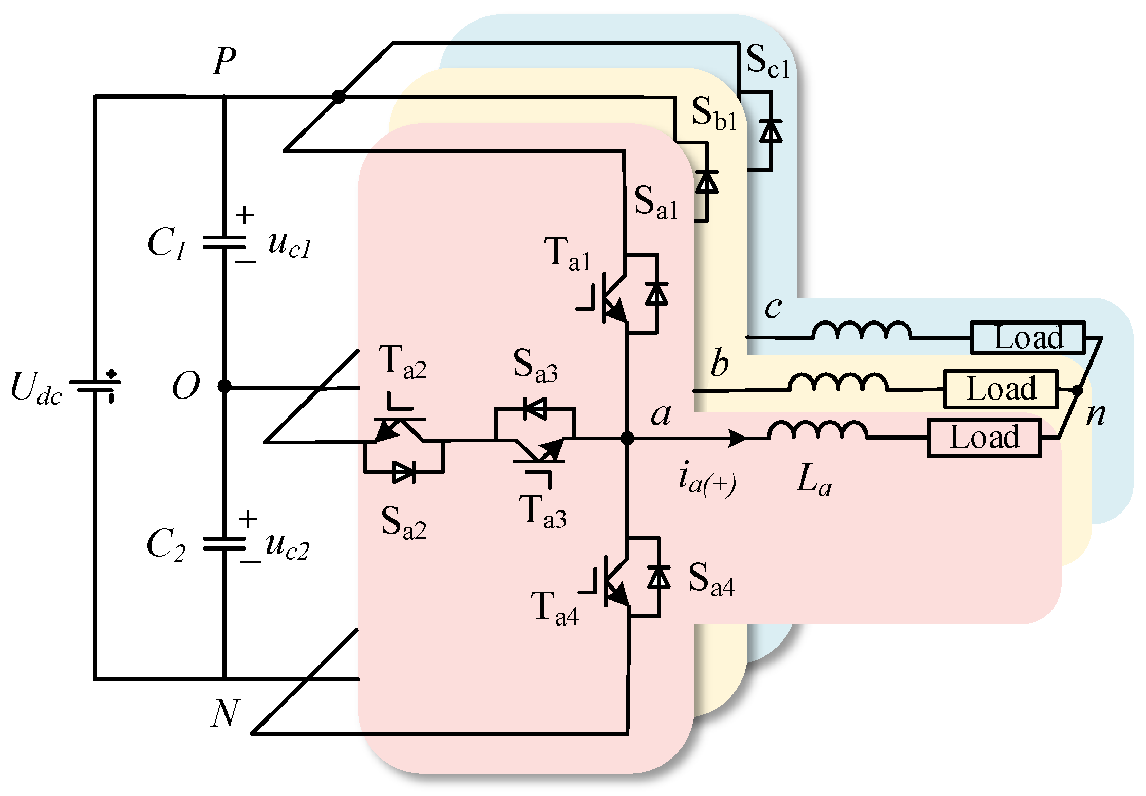
2.1. Hybrid Logic Dynamic Model of the T²3L Inverter

The topology of the ${\mathrm{T}}^{2}3\mathrm{L}$ inverter is shown in Figure 1. ${\mathrm{U}}_{\mathrm{dc}}$ denotes the DC side voltage, where $C_1$ and $C_2$ are the DC-link capacitors. Point O represents the midpoint of the DC bus, serving as the neutral point. Each phase of the inverter consists of four power switches $T_{xi}\left(x=a,b,c;i=1,2,3,4\right)$ along with their corresponding anti-parallel diodes. Where $T_{x1}$ and $T_{x4}$ are connected to the positive and negative terminal of the DC bus respectively, referred to as bridge arm switches; $T_{x2}$ and $T_{x3}$ connect the neutral point O and the output point x, referred to as midpoint switches. The inverter’s output current is filtered through inductor L before being delivered to the resistive load.

The unique topology of the ${\mathrm{T}}^{2}3\mathrm{L}$ inverter creates a pronounced asymmetry in voltage stress distribution. Specifically, the bridge-arm switches withstand the full DC-link voltage (${\mathrm{U}}_{\mathrm{dc}}$), while the neutral-point switches are subjected to only half the voltage ($0.5{\mathrm{U}}_{\mathrm{dc}}$). During positive/negative voltage output generation, its single-device conduction mechanism significantly reduces conduction losses. This advantage contrasts sharply with conventional NPC inverters, which require multiple series-connected devices for the same operation. However, the high voltage rating of the arm switches introduces substantial switching losses. This issue is particularly pronounced under high-voltage operating conditions, significantly degrading the system’s overall efficiency. Consequently, the T-type topology demonstrates efficiency advantages primarily in low-voltage applications. In such scenarios, the optimized conduction losses effectively offset the penalties from switching losses.

Depending on Figure 1, the system’s state equation can be expressed as:

$$\begin{array}{c}\hfill \left\{\begin{array}{c}{u}_{\mathrm{an}}=R{i}_{\mathrm{a}}+L{\displaystyle \frac{\mathrm{d}{i}_{\mathrm{a}}}{dt}}\hfill \\ u_{\mathrm{bn}}=R{i}_{\mathrm{b}}+L{\displaystyle \frac{\mathrm{d}{i}_{\mathrm{b}}}{dt}}\hfill \\ u_{\mathrm{cn}}=R{i}_{\mathrm{c}}+L{\displaystyle \frac{\mathrm{d}{i}_{\mathrm{c}}}{dt}}\hfill \end{array}\right.\end{array}$$

(1)

where $u_{\mathrm{an}}$, $u_{\mathrm{bn}}$, $u_{\mathrm{cn}}$ are the three-phase voltages of the inverter.

According to Kirchhoff’s voltage law and the Y-connection, the three-phase voltage takes the form:

$$\begin{array}{c}\hfill \left[\begin{array}{c}{u}_{\mathrm{an}}\\ u_{\mathrm{bn}}\\ u_{\mathrm{cn}}\end{array}\right]={\displaystyle \frac{1}{3}}\left[\begin{array}{ccc}2& -1& -1\\ -1& 2& -1\\ -1& -1& 2\end{array}\right]\left[\begin{array}{c}{u}_{\mathrm{ao}}\\ u_{\mathrm{bo}}\\ u_{\mathrm{co}}\end{array}\right]\end{array}$$

(2)

Define $S_{xi}$ as the switching signal for switch $T_{xi}$, where $S_{xi}=1$ indicates the on-state of the switch, whereas $S_{xi}=0$ indicates the off-state. The positive direction of the specified current is defined as flowing from the DC side to the AC side of the inverter, represented as ${\sigma }_x=1$, while the reverse direction is represented as ${\sigma }_x=0$. Using phase a as a representative case,

Table 1. A-phase switching signal and output voltage.

Switching State				Pole Voltage
${\mathit{S}}_{\mathit{a}\mathbf{1}}$	${\mathit{S}}_{\mathit{a}\mathbf{2}}$	${\mathit{S}}_{\mathit{a}\mathbf{3}}$	${\mathit{S}}_{\mathit{a}\mathbf{4}}$	${\mathit{u}}_{\mathit{ao}}\left({\mathbf{\sigma }}_{\mathit{a}}\mathbf{=}\mathbf{0}\right)$	${\mathit{u}}_{\mathit{ao}}\left({\mathbf{\sigma }}_{\mathit{a}}\mathbf{=}\mathbf{1}\right)$
1	0	1	0	$u_{c1}$	$u_{c1}$
0	1	1	0	0	0
0	1	0	1	−$u_{c2}$	−$u_{c2}$
0	0	0	1	−$u_{c2}$	−$u_{c2}$
0	0	1	0	0	$u_{c1}$
0	1	0	0	−$u_{c2}$	0
1	0	0	0	$u_{c1}$	$u_{c1}$
0	0	0	0	−$u_{c2}$	$u_{c1}$

delineates the relationship between switching signals and output voltage under normal inverter conditions. Here, $u_{c1}$ and $u_{c2}$ represent the terminal voltages of capacitors $C_1$ and $C_2$.

Under normal operating conditions, $u_{ao}$ is derived from the logical relationship among switching states, current direction, and pole voltage, expressed as:

$$u_{ao}={\sigma }_a(S_{a1}{u}_{c1}-{\overline{S}}_{a1}{\overline{S}}_{a3}{u}_{c2})-{\overline{\sigma }}_a(S_{a4}{u}_{c2}-{\overline{S}}_{a2}{\overline{S}}_{a4}{u}_{c1})$$

(3)

Similarly, the pole voltages of the remaining two phases are given by:

$$\begin{array}{cc}\hfill & u_{bo}={\sigma }_b(S_{b1}{u}_{c1}-{\overline{S}}_{b1}{\overline{S}}_{b3}{u}_{c2})-{\overline{\sigma }}_b(S_{b4}{u}_{c2}-{\overline{S}}_{b2}{\overline{S}}_{b4}{u}_{c1})\hfill \\ \hfill & u_{co}={\sigma }_c(S_{c1}{u}_{c1}-{\overline{S}}_{c1}{\overline{S}}_{c3}{u}_{c2})-{\overline{\sigma }}_c(S_{c4}{u}_{c2}-{\overline{S}}_{c2}{\overline{S}}_{c4}{u}_{c1})\hfill \end{array}$$

(4)

According to Equations (2)–(4), the expression for the three-phase voltage is converted to:

$$\begin{array}{c}\hfill \left[\begin{array}{c}{u}_{\mathrm{an}}\\ u_{\mathrm{bn}}\\ u_{\mathrm{cn}}\end{array}\right]={\displaystyle \frac{1}{3}}\left[\begin{array}{ccc}2& -1& -1\\ -1& 2& -1\\ -1& -1& 2\end{array}\right]\left[\begin{array}{c}{\sigma }_a(S_{a1}{u}_{c1}-{\overline{S}}_{a1}{\overline{S}}_{a3}{u}_{c2})-{\overline{\sigma }}_a(S_{a4}{u}_{c2}-{\overline{S}}_{a2}{\overline{S}}_{a4}{u}_{c1})\hfill \\ {\sigma }_b(S_{b1}{u}_{c1}-{\overline{S}}_{b1}{\overline{S}}_{b3}{u}_{c2})-{\overline{\sigma }}_b(S_{b4}{u}_{c2}-{\overline{S}}_{b2}{\overline{S}}_{b4}{u}_{c1})\hfill \\ {\sigma }_c(S_{c1}{u}_{c1}-{\overline{S}}_{c1}{\overline{S}}_{c3}{u}_{c2})-{\overline{\sigma }}_c(S_{c4}{u}_{c2}-{\overline{S}}_{c2}{\overline{S}}_{c4}{u}_{c1})\hfill \end{array}\right]\end{array}$$

(5)

According to Equations (1) and (5), the mixed logic dynamic model of ${\mathrm{T}}^{2}3\mathrm{L}$ inverter under normal operation is described as follows:

$$\begin{array}{c}\hfill \left[\begin{array}{c}{\dot{i}}_{\mathrm{a}}\\ {\dot{i}}_{\mathrm{b}}\\ {\dot{i}}_{\mathrm{c}}\end{array}\right]=-\left[\begin{array}{ccc}{\displaystyle \frac{R}{L}}& 0& 0\\ 0& {\displaystyle \frac{R}{L}}& 0\\ 0& 0& {\displaystyle \frac{R}{L}}\end{array}\right]\left[\begin{array}{c}{i}_{\mathrm{a}}\\ i_{\mathrm{b}}\\ i_{\mathrm{c}}\end{array}\right]+{\displaystyle \frac{1}{3L}}\left[\begin{array}{ccc}2& -1& -1\\ -1& 2& -1\\ -1& -1& 2\end{array}\right]\left[\begin{array}{c}{u}_{ao}\hfill \\ u_{bo}\hfill \\ u_{co}\hfill \end{array}\right]\end{array}$$

(6)

Equation (6) can be further rewritten as:

$$\dot{i}=Ai+Bu$$

(7)

In Equation (7):

$$\dot{i}={\left[{\dot{i}}_a{\dot{i}}_{\mathrm{b}}{\dot{i}}_{\mathrm{c}}\right]}^{\mathrm{T}}u={\left[u_{ao}{u}_{bo}{u}_{co}\right]}^T$$

$$A=diag\left(-{\displaystyle \frac{R}{L}},-{\displaystyle \frac{R}{L}},-{\displaystyle \frac{R}{L}}\right)B={\displaystyle \frac{1}{3L}}\left[\begin{array}{ccc}2& -1& -1\\ -1& 2& -1\\ -1& -1& 2\end{array}\right]$$

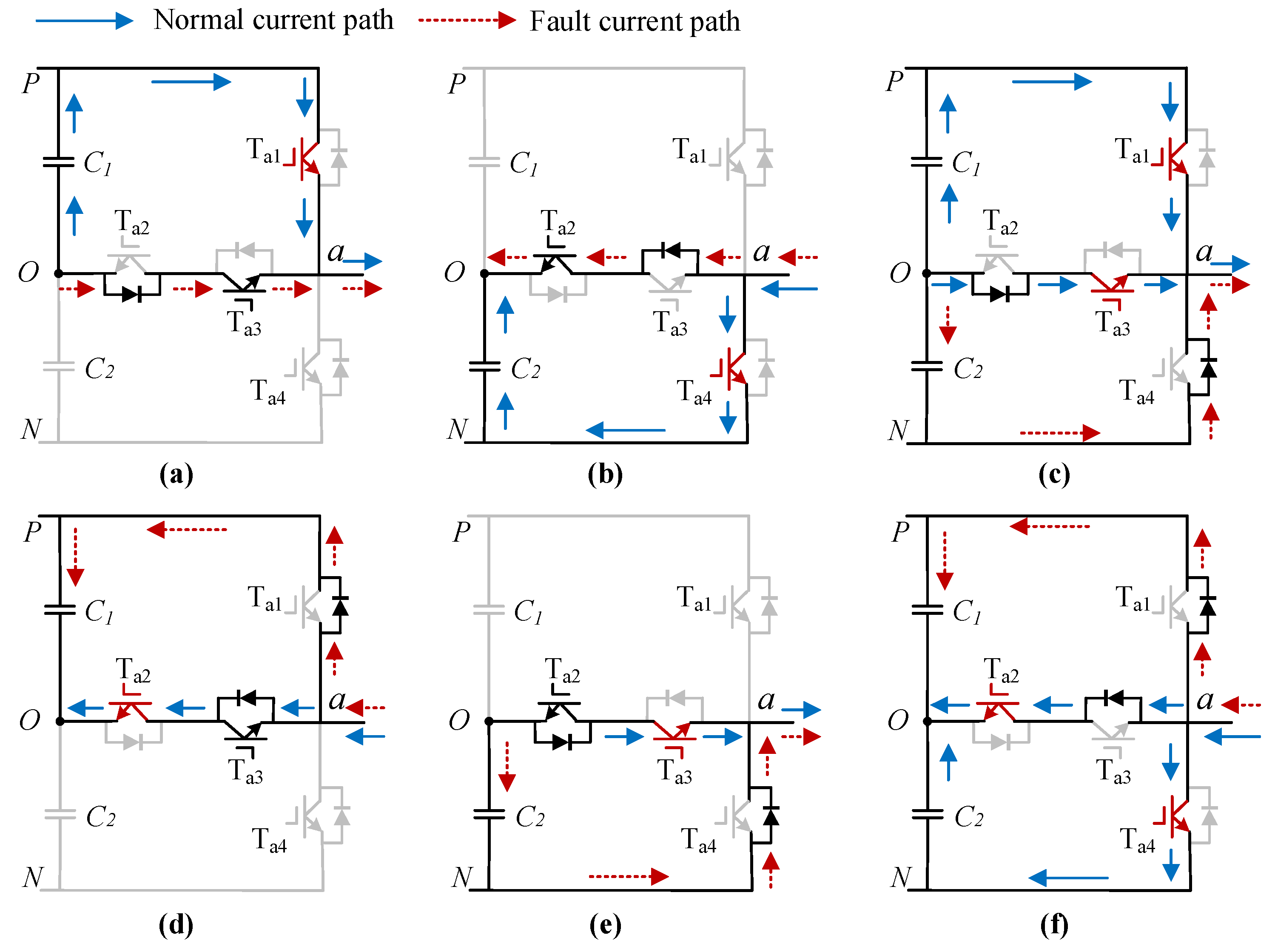
2.2. Analysis of Power Switch Fault

Owing to the topological characteristics of the ${\mathrm{T}}^{2}3\mathrm{L}$ inverter, each phase bridge arm can produce three distinct voltage states by combining power switches. When the output voltages of the bridge arm are $+0.5{\mathrm{U}}_{\mathrm{dc}}$, 0, and $-0.5{\mathrm{U}}_{\mathrm{dc}}$ respectively, it corresponds to the operating state [P], [O] and [N], as detailed in

Table 2. Pole voltage and operating state.

Switching State	Pole Voltage	Operating State
1 , 0 , 1 , 0	$+0.5U_{dc}$	[P]
0 , 1 , 1 , 0	0	[O]
0 , 1 , 0 , 1	−$0.5U_{dc}$	[N]

.

When OC faults occur in single or multiple power switches, the inverter’s outputs will be distorted to variable degrees. Such faults significantly degrade inverter performance and may compromise the operational safety of the entire system. In practical engineering scenarios, simultaneous OC faults involving three or more power switches are extremely rare. Considering the low frequency of this phenomenon, this section focuses on analyzing the single- and double-switch faults in phase a. Single-switch faults are further categorized into bridge-arm switch faults and midpoint switch faults. The current paths before and after fault occurrence are illustrated in Figure 2. Blue traces correspond to steady-state current distribution, whereas red traces delineate fault-induced abnormal conduction paths.

($1)$ OC faults in the bridge-arm switches: Figure 2a demonstrates that during state [P] operation with $I_{\mathrm{a}}>0$, an OC fault occurring in $T_{a1}$ alters the current path. The forward current flows through $T_{a3}$ and $D_{a2}$ instead of $T_{a1}$, thereby maintaining freewheeling operation. At this point, the positive half-cycle of the current is significantly distorted, while voltage $u_{ao}$ drops to zero. Under state [P] operation with $I_{\mathrm{a}}<0$, an OC fault in switch $T_{a1}$ maintains the original current path and preserves pole voltage stability at $+0.5{\mathrm{U}}_{\mathrm{dc}}$. The fault has no negative influence on the circuit within a short period. As shown in Figure 2b, the faults in $T_{a4}$ exhibit similar characteristics. When the OC fault occurs, the current’s negative half-cycle becomes severely distorted, and the pole voltage also drops to zero.

($2)$ OC faults in the midpoint switches: As shown in Figure 2d, during the inverter’s operation in state [O], the OC fault develops in $T_{a2}$. This changes the negative current path through $T_{a2}$, forcing it to reroute via $D_{a1}$ to facilitate freewheeling. At this time, the current’s negative half-cycle shows slight distortion, while voltage $u_{ao}$ rises to $+0.5{\mathrm{U}}_{\mathrm{dc}}$. The current paths before and after the OC fault in another midpoint switch ($T_{a3}$) are depicted in Figure 2e. Meanwhile, the positive half of the current is slightly distorted, and $u_{ao}$ drops from 0 to $-0.5{\mathrm{U}}_{\mathrm{dc}}$.

($3)$ OC faults in the positive/negative level switches: During the inverter’s state [P] operation and $I_{\mathrm{a}}>0$, the positive-level switches ($T_{a1}$ and $T_{a3}$) experience an OC fault, as illustrated in Figure 2c. The current flows through $D_{a4}$ for freewheeling, with only state [N] of the inverter phase remaining normal. Consequently, the current conducts during the negative half cycle, and $u_{ao}$ changes to $-0.5{\mathrm{U}}_{\mathrm{dc}}$. The current paths before and after the fault of the negative-level switches ($T_{a2}$ and $T_{a4}$) are illustrated in Figure 2f. In this case, only state [P] of phase a is normal, restricting current conduction to the positive half cycle. Consequently, the pole voltage changes to $+0.5{\mathrm{U}}_{\mathrm{dc}}$.

3. Open-Circuit Fault Diagnosis Strategy

The proposed method is presented in Figure 3, and its core architecture consists of fault detection and location. Firstly, the IASMO is constructed through the hybrid logic dynamic model. Current characteristic values are extracted separately from the estimated currents and actual inverter outputs. These values construct fault detection variables and adaptive thresholds, enabling real-time fault detection via dynamic thresholding. Secondly, the initial location variables narrow down the fault range to the positive/negative level switches. Then, the fault location variables facilitate accurate identification of the faulty switches, achieving precise diagnosis in ${\mathrm{T}}^{2}3\mathrm{L}$ inverters.

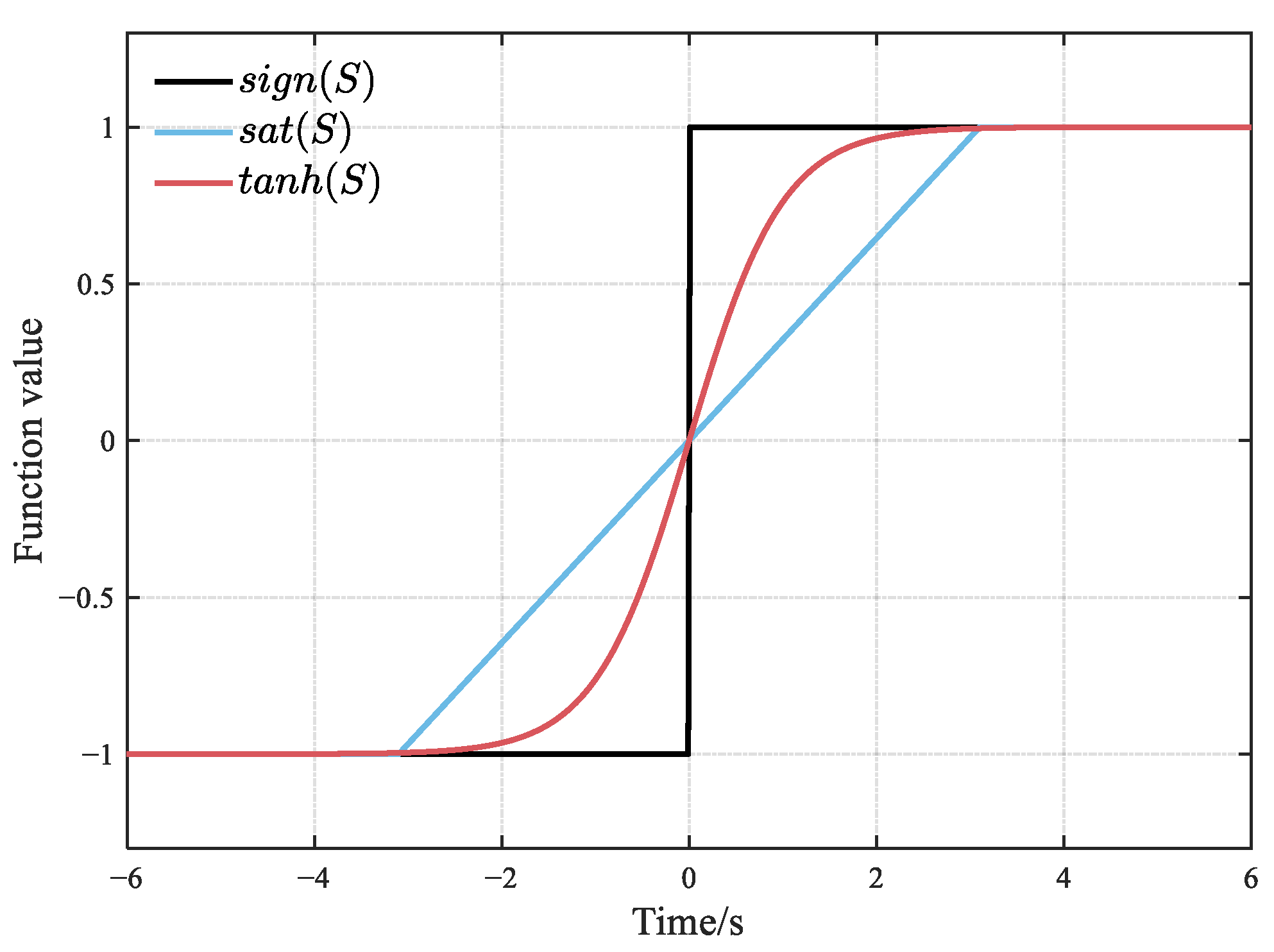
3.1. Design of IASMO

In practical inverter systems where unavoidable unknown disturbances inherently exist, the model under normal working condition is formulated as:

$$\begin{array}{c}\hfill \left\{\begin{array}{c}\dot{i}=Ai+Bu+Ev\hfill \\ y=Ci\hfill \end{array}\right.\end{array}$$

(8)

where $i\in {\Re }^3$ represents the state variable, $y\in {\Re }^3$ is the output variable, u is the three-phase output voltage, v represents unknown interference signal, bounded with known upper and lower bounds. It satisfies the constraint $∥v∥<\lambda$, $\lambda >0$. C and E are three-dimensional identity matrices.

The IASMO is designed according to Equation (8) as follows:

$$\begin{array}{c}\hfill \left\{\begin{array}{c}\dot{\widehat{i}}=A\widehat{i}+Bu+L\left(C\widehat{i}-y\right)+f\left(S\right)\hfill \\ \widehat{y}=C\widehat{i}\hfill \end{array}\right.\end{array}$$

(9)

where $\widehat{i}$ represents the estimated current, L denotes the gain matrix, $S=C\widehat{i}-y$ represents the sliding mode surface. $f\left(S\right)$ denotes the adaptive reaching law, defined as follows:

$$f\left(S\right)=-{\displaystyle \frac{k}{Q\left(S\right)}}tanh\left(\alpha S\right)$$

(10)

where k denotes the observer gain. It satisfies $k\ge \gamma \lambda +\gamma \rho$, where $\rho$ is a positive constant. The switching function adopts the hyperbolic tangent function, expressed as follows:

$$tanh\left(\alpha S\right)={\displaystyle \frac{e^{\alpha S}-e^{-\alpha S}}{e^{\alpha S}+e^{-\alpha S}}}$$

(11)

where $\alpha >0$.

Traditional sliding mode observers typically utilize the sign function or the saturation function as the switching function. Among these, the sign function is discontinuous at the switching point and notoriously induces high-frequency chattering. Although the saturation function smooths the switching process through the boundary layer, it remains approximately equivalent to the sign function outside this region. Furthermore, designing the boundary layer thickness requires balancing convergence speed and chattering intensity. Figure 4 shows the curves of the conventional switching function and the hyperbolic tangent function. Compared with the above switching functions, the hyperbolic tangent function naturally reduces chattering due to its smooth transition characteristics. This reduces the effect of environmental changes on current tracking accuracy.

The adaptive term in Equation (10) is represented as:

$$Q\left(S\right)=\gamma +\left(1-\gamma \right)\left(1-{\displaystyle \frac{2}{\pi }}arctan\left|S\right|\right)$$

(12)

where $0<\gamma <1$.

When the trajectory of the state variable $\widehat{i}$ deviates significantly from the sliding mode surface, $k/\phantom{kQ\left(S\right)}Q\left(S\right)$ asymptotically converges to $k/\phantom{k\gamma }\gamma$, thereby guaranteeing $k/\phantom{kQ\left(S\right)}Q\left(S\right)>k$. This gain elevation in $k/\phantom{kQ\left(S\right)}Q\left(S\right)$ accelerates the state trajectory’s convergence toward the sliding mode surface, effectively minimizing the reaching time. As the trajectory of the state variable $\widehat{i}$ approaches the sliding mode surface, where $\left|S\right|$ tends to zero, $k/\phantom{kQ\left(S\right)}Q\left(S\right)$ converges to k. This adaptive reduction in $k/\phantom{kQ\left(S\right)}Q\left(S\right)$ effectively suppresses chattering in the observer.

Theorem 1. 

If there exists a positive definite symmetric matrix $P\in {\Re }^{3\times 3}$ and a matrix Z such that the following inequality holds:

$$A^{\mathrm{T}}P+PA-C^{\mathrm{T}}{Z}^{\mathrm{T}}-ZC<0$$

(13)

Under these conditions, the observer error dynamics are asymptotically stable, and the error dynamics are described by the following equation:

$$\dot{e}=(A-LC)e+Ev-f\left(S\right)$$

(14)

where $e=i-\widehat{i}$, and $L=P^{-1}Z$.

Proof of Theorem 1. 

The Lyapunov function is constructed as follows:

$$V=e^{\mathrm{T}}Pe$$

(15)

Differentiating the above equation yields:

$$\begin{array}{c}\hfill \begin{array}{cc}\hfill \dot{V}& ={\dot{e}}^{\mathrm{T}}Pe+e^{\mathrm{T}}P\dot{e}\hfill \\ & =[e^{\mathrm{T}}{(A-LC)}^{\mathrm{T}}+v^{\mathrm{T}}{E}^{\mathrm{T}}-f^T\left(S\right)]Pe+e^{\mathrm{T}}P[(A-LC)e+Ev-f\left(S\right)]\hfill \\ & =e^{\mathrm{T}}[{(A-LC)}^{\mathrm{T}}P+P(A-LC)]e+2v^{\mathrm{T}}{E}^{\mathrm{T}}Pe-2f^T\left(S\right)Pe\hfill \end{array}\end{array}$$

(16)

Based on the Cauchy-Schwarz inequality and norm properties, the following inequality holds:

$$\begin{array}{c}\hfill \begin{array}{cc}\hfill \dot{V}& \le e^{\mathrm{T}}[{(A-LC)}^{\mathrm{T}}P+P(A-LC)]e+2∥Pe∥\left(∥E∥\lambda -{\displaystyle \frac{k}{\gamma }}\right)\hfill \\ & \le e^{\mathrm{T}}[{(A-LC)}^{\mathrm{T}}P+P(A-LC)]e-2\rho ∥Pe∥\hfill \\ & \le e^{\mathrm{T}}[{(A-LC)}^{\mathrm{T}}P+P(A-LC)]e\hfill \\ & \le e^{\mathrm{T}}[A^{\mathrm{T}}P-C^{\mathrm{T}}{\left(P^{-1}Z\right)}^{\mathrm{T}}P+PA-P{P}^{-1}ZC]e\hfill \\ & \le e^{\mathrm{T}}[A^{\mathrm{T}}P+PA-C^{\mathrm{T}}{Z}^{\mathrm{T}}-ZC]e\hfill \end{array}\end{array}$$

(17)

As demonstrated above, if the inequality $A^{\mathrm{T}}P+PA-C^{\mathrm{T}}{Z}^{\mathrm{T}}-ZC<0$ holds, then $\dot{V}<0$. This implies that the observer error is asymptotically stable. Consequently, the designed IASMO is also asymptotically stable. □

Notably, the positive definite symmetric matrix P, matrix Z, and the condition $A^{\mathrm{T}}P+PA-C^{\mathrm{T}}{Z}^{\mathrm{T}}-ZC<0$ can be addressed with the Linear Matrix Inequality (LMI) toolbox.

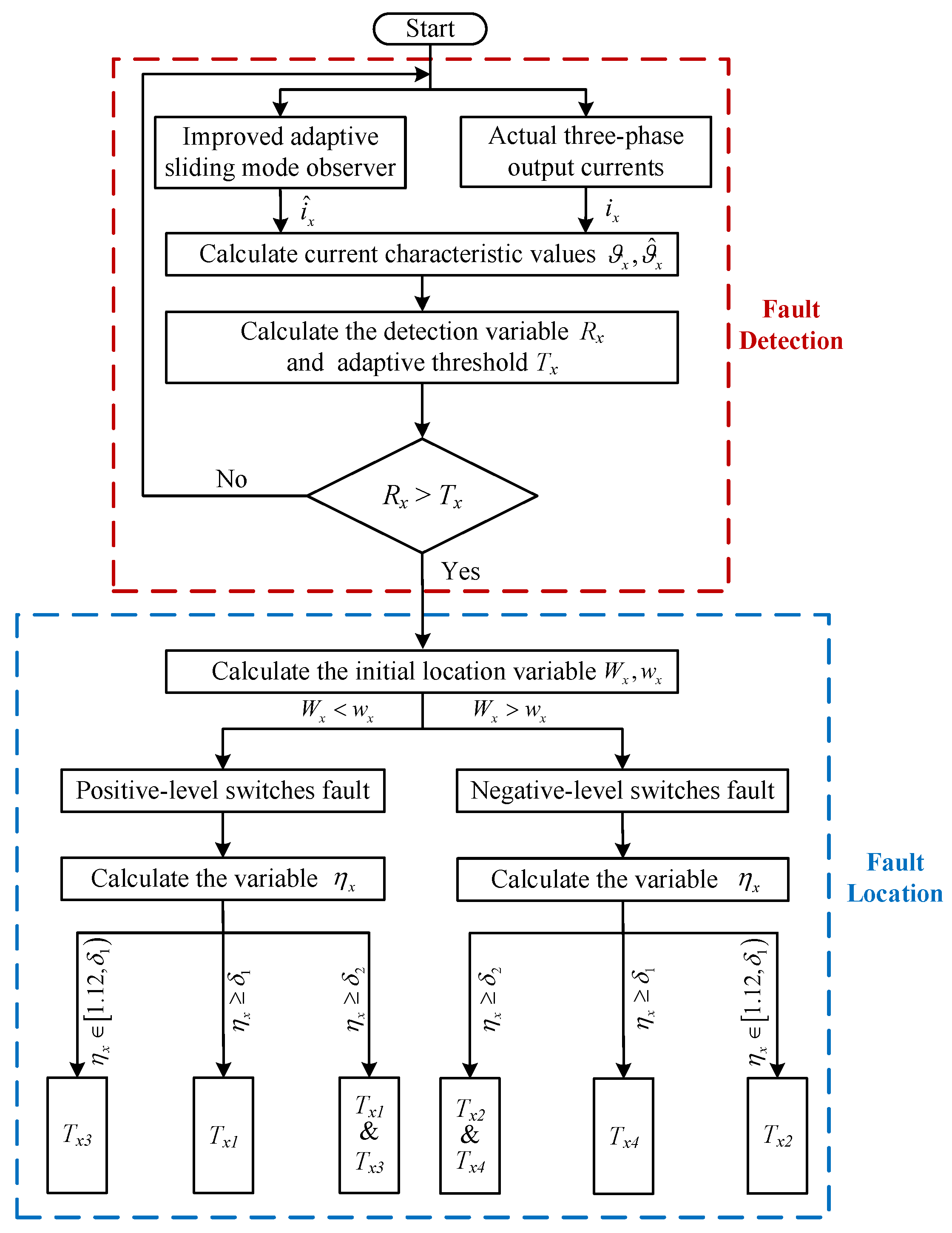
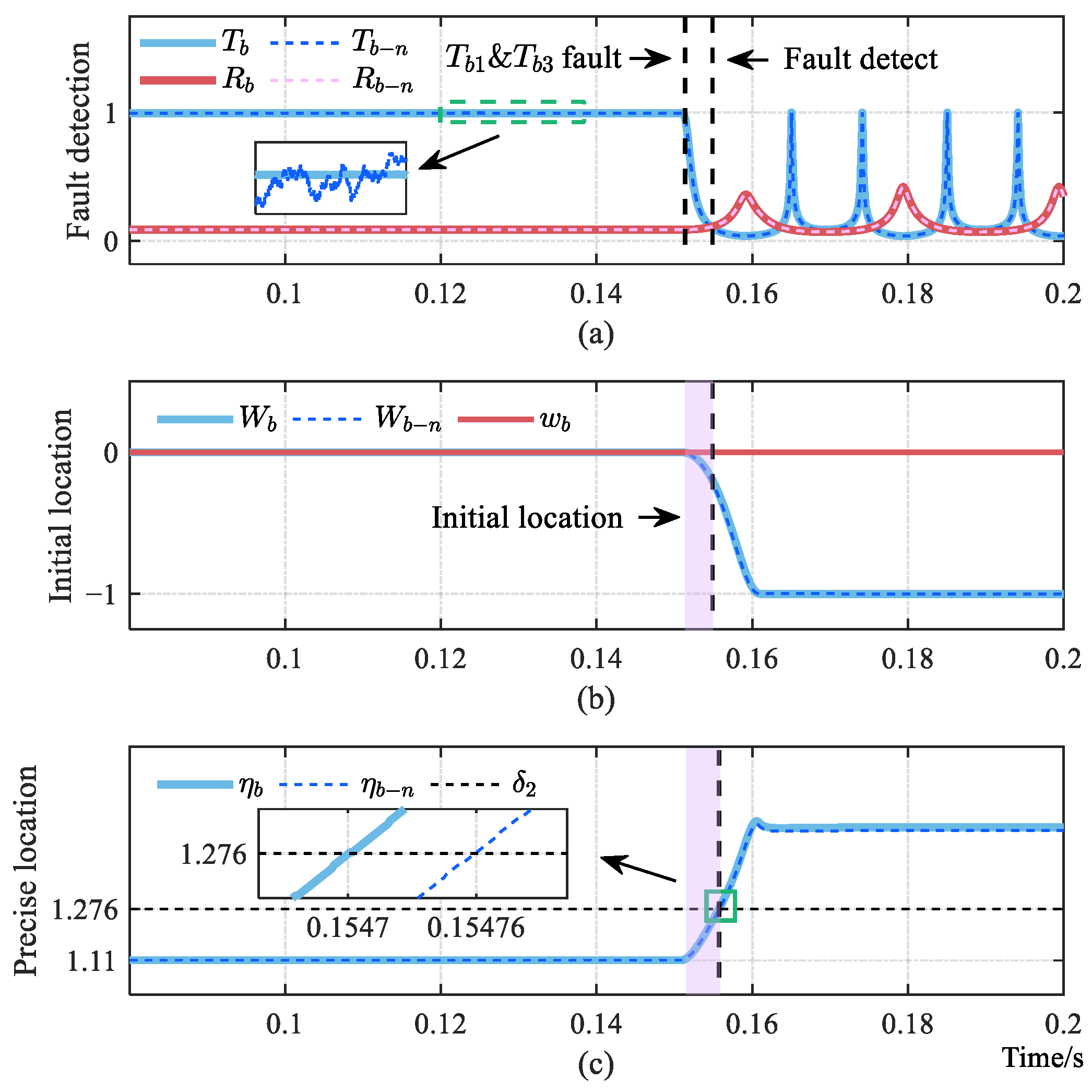
3.2. Fault Detection

Under normal operating conditions, the output current of the ${\mathrm{T}}^{2}3\mathrm{L}$ inverter closely matches the current estimated by the IASMO. However, the emergence of OC faults induces a substantial deviation between the inverter’s actual output current and the observer-estimated value, leading to a mismatch between the two. Leveraging this distinctive current divergence phenomenon, this section establishes current characteristic values to quantitatively characterize the discrepancy mechanism. A fault detection variable and an adaptive threshold are then constructed accordingly. By comparing the detection variable with the threshold, the proposed method enables highly accurate detection of OC faults.

According to the analysis of OC faults in ${\mathrm{T}}^{2}3\mathrm{L}$ inverters, power switch faults result in distortion of the output current. Exploiting these distortion characteristics, this paper proposes a fault detection variable $R_x$ and an adaptive threshold $T_x$, defined as:

$$R_x={\displaystyle \frac{arsinh\left({\vartheta }_x\right)}{{\vartheta }_x}}$$

(18)

$$T_x={\displaystyle \frac{arsinh\left(\left|{\widehat{\vartheta }}_x-{\vartheta }_x\right|\right)}{\left|{\widehat{\vartheta }}_x-{\vartheta }_x\right|}}$$

(19)

where ${\vartheta }_x$ and ${\widehat{\vartheta }}_x$ denote the actual and estimated current characteristic values, as follows:

$${\vartheta }_x={\left({\displaystyle \frac{1}{\tau }}{\int }_{t-\tau }^t{\left|i_x\right|}^{2}dt\right)}^{1/2},{\widehat{\vartheta }}_x={\left({\displaystyle \frac{1}{\tau }}{\int }_{t-\tau }^t{\left|{\widehat{i}}_x\right|}^{2}dt\right)}^{1/2}$$

(20)

Here, $\tau$ denotes half of the fundamental current period. This definition of ${\vartheta }_x$ aims to reduce the influence of peak currents and harmonics, ensuring robust fault detection.

The adaptive behavior of the threshold $T_x$ is guaranteed by the mathematical properties of the inverse hyperbolic sine function ($arsinh$). For any $x>0$, there exists a strict inequality:

$${\displaystyle \frac{x}{1+x}}<arsinh\left(x\right)<x$$

(21)

Combining the above Equations (18), (19) and (21), when the inverter operates normally, the observed current value is highly consistent with the actual output value, meaning that $\left|{\widehat{\vartheta }}_x-{\vartheta }_x\right|\to 0^{+}$. In this case, the fault detection variable and adaptive threshold satisfy the following expressions respectively:

$$R_x={\displaystyle \frac{arsinh\left({\vartheta }_x\right)}{{\vartheta }_x}}\in \left(0,1\right)$$

(22)

$$T_x=\underset{\left|{\widehat{\vartheta }}_x-{\vartheta }_x\right|\to 0^{+}}{lim}{\displaystyle \frac{arsinh\left(\left|{\widehat{\vartheta }}_x-{\vartheta }_x\right|\right)}{\left|{\widehat{\vartheta }}_x-{\vartheta }_x\right|}}\approx 1$$

(23)

As demonstrated by the equations above, under this condition, the detection variable $R_x$ remains consistently below the threshold $T_x$. However, upon the occurrence of an OC fault in the inverter, $\left|{\widehat{\vartheta }}_x-{\vartheta }_x\right|$ will increase, resulting in a corresponding alteration of the threshold $T_x$, and the detection variable $R_x$ will rapidly exceed the existing threshold. Therefore, the proposed detection method achieves reliable OC fault identification through real-time monitoring of the detection variable-threshold relationship.

3.3. Fault Location

As previously analyzed, both single-switch and double-switch faults within the same phase are indicated by $R_x$ exceeding $T_x$. Therefore, the fault detection variables can only detect and isolate faulty branches, rather than pinpoint the specific faulty switches. This paper performs initial location using variables $W_x$ and $w_x$, and incorporates ${\eta }_x$ to precisely identify faulty switches.

First, taking into account the distinct characteristics of the observed and actual currents, the initial location variables are introduced to distinguish between positive- and negative-level switches. Their specific representations are as follows:

$$W_x={\displaystyle \frac{{\int }_{t-T}^t{i}_{x}dt}{{\int }_{t-T}^t\left|i_x\right|dt}},w_x={\displaystyle \frac{{\int }_{t-T}^t{\widehat{i}}_{x}dt}{{\int }_{t-T}^t\left|{\widehat{i}}_x\right|dt}}$$

(24)

According to the preceding analysis of switch OC faults, $W_x=w_x$ under normal inverter operation, $W_x<w_x$ when the positive-level switches ($T_{x1}$ and $T_{x3}$) fault, $W_x>w_x$ during the negative-level switches ($T_{x2}$ and $T_{x4}$) fail. To accurately determine the location of the faulty switches, the fault location variable ${\eta }_x$ is introduced as follows:

$${\displaystyle {\eta }_x=\frac{{\left({\displaystyle \frac{1}{T}{\int }_{t-T}^t{\left|i_x\right|}^{2}dt}\right)}^{1/2}}{{\displaystyle \frac{1}{T}{\int }_{t-T}^t\left|i_x\right|dt}}}$$

(25)

Under normal or steady-state operation, the location variable ${\eta }_x$ remains stabilized at approximately 1.11. In ${\mathrm{T}}^{2}3\mathrm{L}$ inverters, faults in the bridge-arm switches and midpoint switches affect the output current to different degrees.A fault in midpoint switch ($T_{x2}$ or $T_{x3}$) causes a slight current attenuation, resulting in ${\eta }_x\in \left[1.11,{\eta }_1\right]$,where ${\eta }_1$ denotes the maximum value of ${\eta }_x$ under this condition. A fault in bridge-arm switch ($T_{x1}$ or $T_{x4}$) leads to significant current attenuation, corresponding to ${\eta }_x\in \left[1.11,{\eta }_2\right]$ with ${\eta }_2>{\eta }_1$. Due to partial overlap between the characteristic ranges of the two fault types, a classification threshold ${\delta }_1=1.002\times {\eta }_1$ is designed to enhance identification accuracy. Midpoint switch faults are detected when ${\eta }_x\in \left[1.11,{\delta }_1\right)$, whereas ${\eta }_x\ge {\delta }_1$ indicates the bridge-arm switch faults. To improve robustness under practical disturbances such as noise, the identification interval for midpoint switch faults is narrowed to ${\eta }_x\in \left[1.12,{\delta }_1\right)$.

The above method is applicable to scenarios with partial double-switch faults in the same phase. The distinctive topology of the ${\mathrm{T}}^{2}3\mathrm{L}$ inverter results in the complete disappearance of the forward current when both positive-level switches ($T_{x1}$ and $T_{x3}$) fail simultaneously. This phenomenon leads to a pronounced increase in ${\eta }_x$. In this case, the positioning variable satisfies ${\eta }_x\in \left[1.11,{\eta }_3\right]$, where ${\eta }_3>{\eta }_2$. Similarly, when both $T_{x2}$ and $T_{x4}$ experience simultaneous faults, ${\eta }_x$ also falls within the range ${\eta }_x\in \left[1.11,{\eta }_3\right]$. Therefore, a threshold value of ${\delta }_2=1.002\times {\eta }_2$ is defined to differentiate this case from other fault conditions. When ${\eta }_x\ge {\delta }_2$, it indicates either concurrent faults of $T_{x1} \& T_{x3}$ or concurrent faults of $T_{x2} \& T_{x4}$. Based on the preceding analysis, the fault location criteria for the ${\mathrm{T}}^{2}3\mathrm{L}$ inverter are defined in Equation (26):

$$F_{xi}=\left\{\begin{array}{cc}{T}_{x1},\hfill & W_x<w_x\&{\eta }_x\ge {\delta }_1\hfill \\ T_{x4},\hfill & W_x>w_x\&{\eta }_x\ge {\delta }_1\hfill \\ T_{x2},\hfill & W_x>w_x\&{\eta }_x\in \left[1.12,{\delta }_1\right)\hfill \\ T_{x3},\hfill & W_x<w_x\&{\eta }_x\in \left[1.12,{\delta }_1\right)\hfill \\ T_{x1}\&T_{x3},\hfill & W_x<w_x\&{\eta }_x\ge {\delta }_2\hfill \\ T_{x2}\&T_{x4},\hfill & W_x>w_x\&{\eta }_x\ge {\delta }_2\hfill \end{array}\right.$$

(26)

where, $F_{xi}$ represents the faulty switches.

4. Simulation Verification and Physical Experiment

To validate the effectiveness and robustness of the proposed method, the ${\mathrm{T}}^{2}3\mathrm{L}$ inverter system and the proposed approach were modeled and simulated in Simulink. The specific system parameters are presented in

Table 3. Main parameters of ${\mathrm{T}}^{2}3\mathrm{L}$ inverter.

Parameter	Value
DC side voltage ${\mathrm{U}}_{\mathrm{dc}}$	$300\mathrm{V}$
DC side capacitance $C_1,C_2$	$5.6\ast 10^{-3}\mathrm{F}$
Sampling time $T_s$	$10^{-6}\mathrm{s}$
Three-phase filter inductance L	$6\ast 10^{-3}\mathrm{H}$
Three-phase load resistance R	$8.3\Omega$

.

4.1. Observer Stability Verification

Additionally, based on the parameters provided in Table 3 and Theorem 1, the corresponding calculations were carried out using the LMI toolbox in Matlab, yielding the following results:

$$P={10}^5\left(\begin{array}{ccc}4.1336& 0& 0\\ 0& 4.1336& 0\\ 0& 0& 4.1336\end{array}\right)$$

(27)

$$Z={10}^8\left(\begin{array}{ccc}-5.7161& 0& 0\\ 0& -5.7161& 0\\ 0& 0& -5.7161\end{array}\right)$$

(28)

Accordingly, there exist a positive definite symmetric matrix P and a matrix Z satisfying condition $A^{\mathrm{T}}P+PA-C^{\mathrm{T}}{Z}^{\mathrm{T}}-ZC<0$, thus ensuring the asymptotic stability of the designed IASMO.

Furthermore, the fault location threshold is determined by the maximum value of ${\eta }_x$ under the three switch fault conditions. Through multiple simulation experiments, the values of ${\eta }_1$, ${\eta }_2$, and ${\eta }_3$ were determined to be 1.163, 1.274, and 1.561, respectively. Therefore, location thresholds ${\delta }_1$ and ${\delta }_2$ are set to 1.165 and 1.276. The criteria for locating faulty switches are detailed as follows:

$$F_{xi}=\left\{\begin{array}{cc}{T}_{x1},\hfill & W_x<w_x\&{\eta }_x\ge 1.165\hfill \\ T_{x4},\hfill & W_x>w_x\&{\eta }_x\ge 1.165\hfill \\ T_{x2},\hfill & W_x>w_x\&{\eta }_x\in \left[1.12,1.165\right)\hfill \\ T_{x3},\hfill & W_x<w_x\&{\eta }_x\in \left[1.12,1.165\right)\hfill \\ T_{x1}\&T_{x3},\hfill & W_x<w_x\&{\eta }_x\ge 1.276\hfill \\ T_{x2}\&T_{x4},\hfill & W_x>w_x\&{\eta }_x\ge 1.276\hfill \end{array}\right.$$

(29)

4.2. Method Validity Verification

This section validates the effectiveness of the proposed method under conditions involving single-switch faults and partial same-phase double-switch faults.

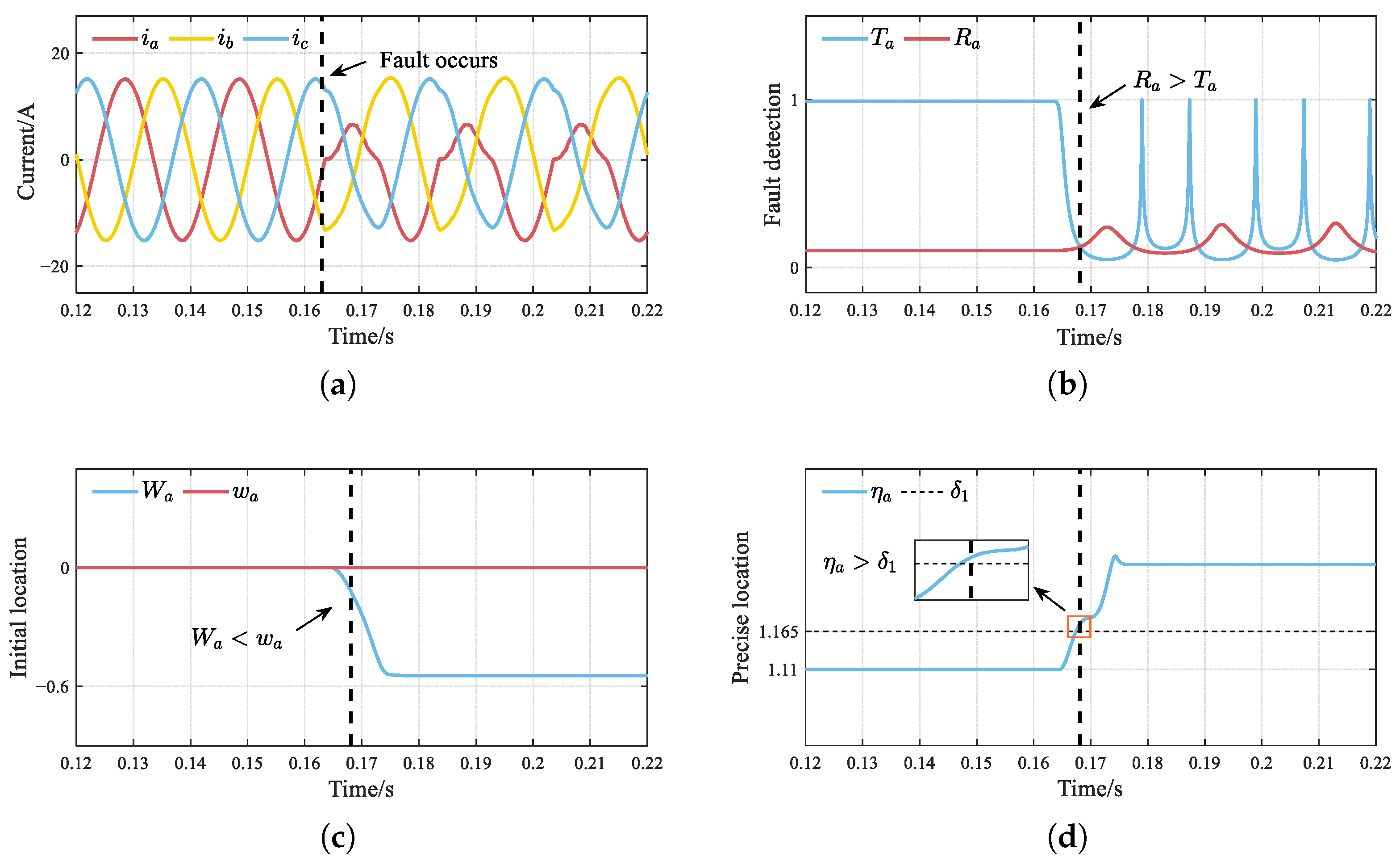
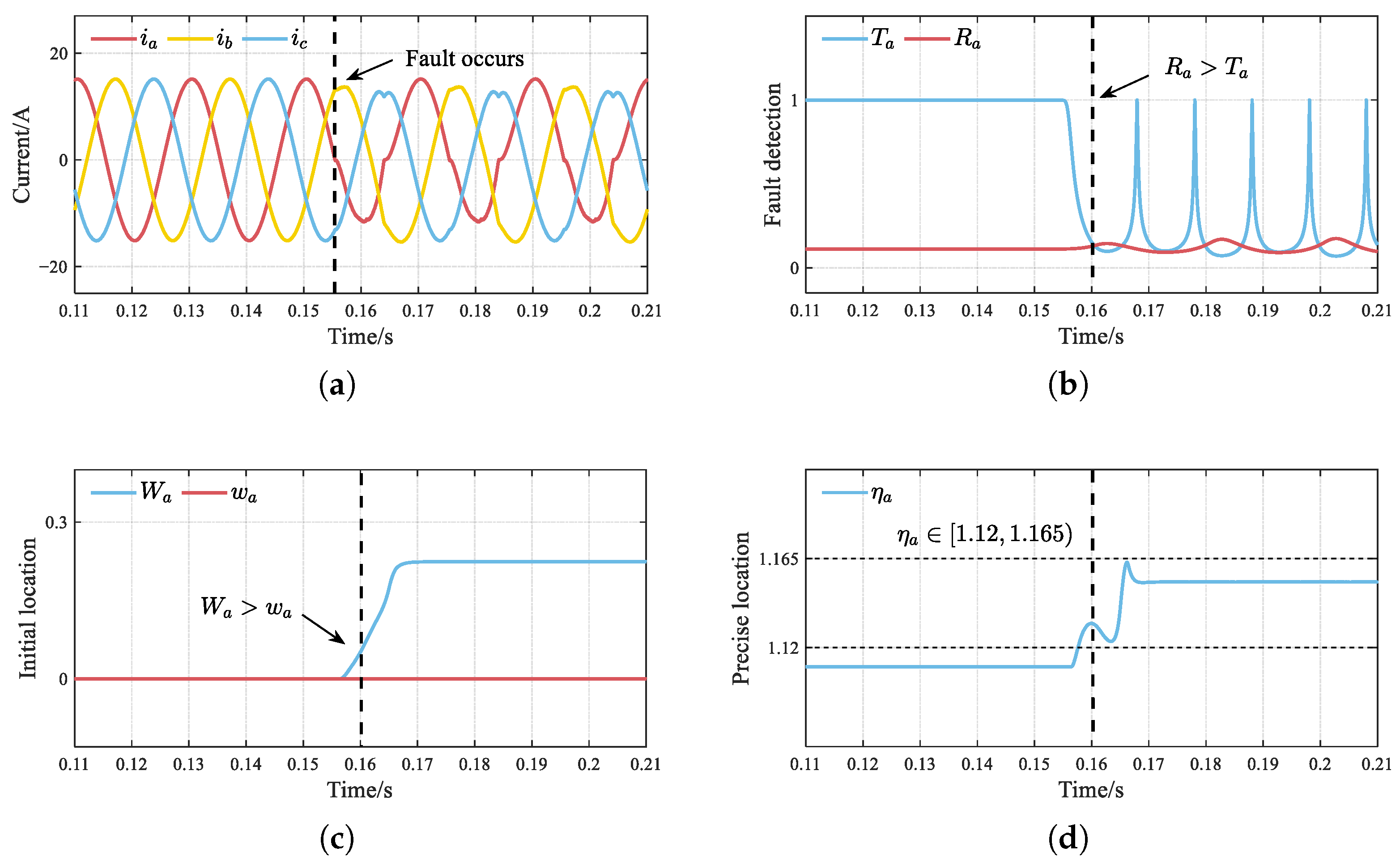
4.2.1. Experimental Results of Single-Switch Fault

Figure 5 illustrates the diagnostic results when an OC fault occurs in $T_{a1}$. As shown in the figure, when the inverter is operating normally, it generates a three-phase sinusoidal current with an amplitude of 15 A and a frequency of 50 Hz. The fault detection variable $R_a$ is consistently lower than the adaptive threshold $T_a$, with the initial location variable satisfying $W_a=w_a$, while ${\eta }_a$ maintains a value of 1.11. An OC fault occurs in $T_{a1}$ at $t=0.163$ s. Concurrent with the pronounced phase-a positive current attenuation, all three-phase outputs manifest heterogeneous harmonic distortion characteristics. The detection variable $R_a$ exceeds the threshold $T_a$ within $22\%$ of the fundamental current period following the fault. Meanwhile, $W_a<w_a$ suggests a fault in positive-level switches ($T_{a1}$ and $T_{a3}$). Combined with ${\eta }_a\ge 1.165$, an OC fault in $T_{a1}$ is conclusively identified.

Figure 6 presents the diagnostic results when $T_{a2}$ has an OC fault. After the fault occurs, the negative phase current of phase a exhibits a slight decay. The fault detection variable $R_a$ gradually increases until exceeding the threshold $T_a$, thereby identifying phase a as the faulty phase. Additionally, the positioning variable $W_a>w_a$ indicates a fault in the negative-level switches ($T_{a2}$ and $T_{a4}$). Since ${\eta }_a$ varied yet consistently remained within the range of $\left[1.12,1.165\right)$, it is ultimately determined that $T_{a2}$ is faulty.

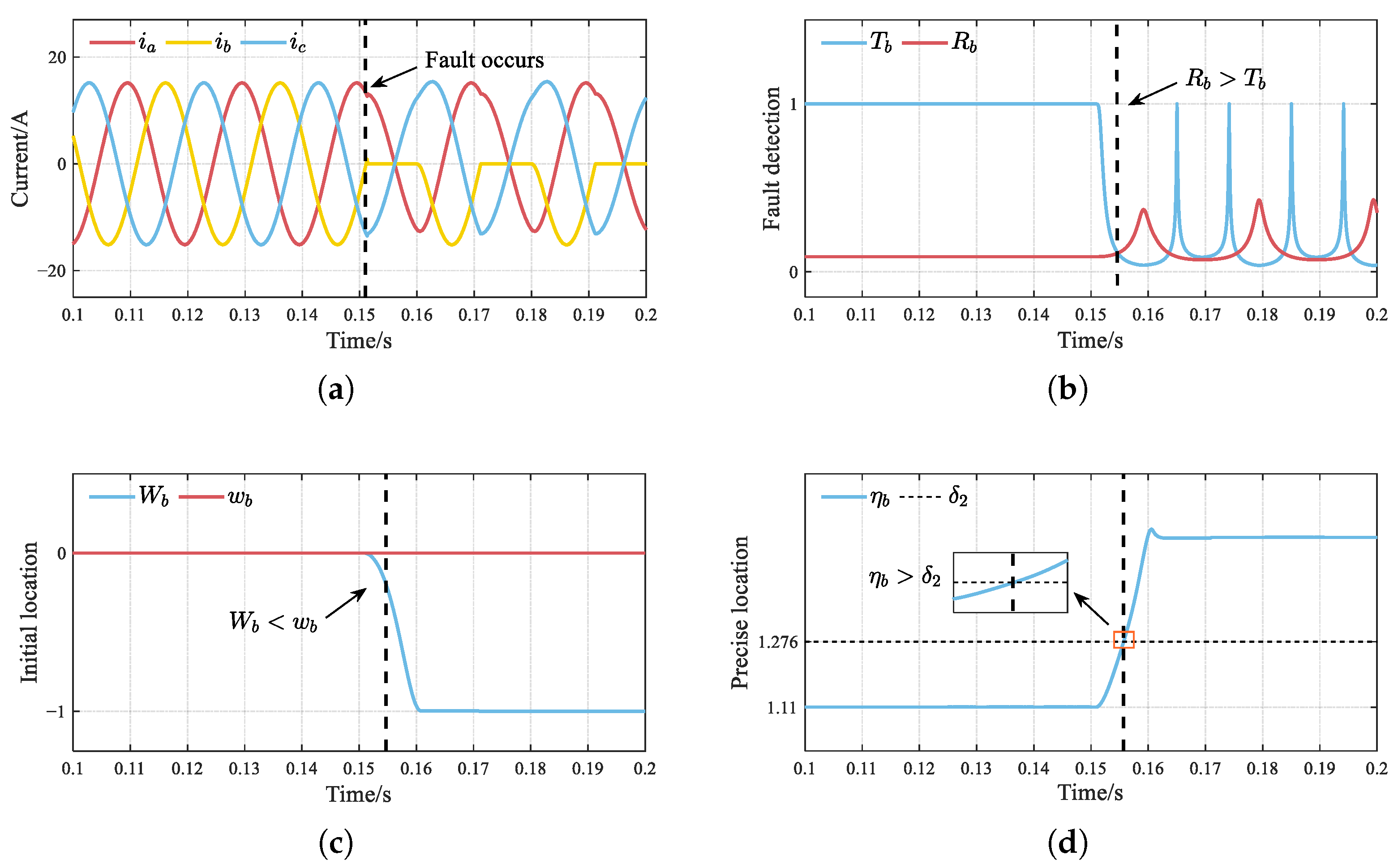
4.2.2. Experimental Results of Same-Phase Double-Switch Fault

Figure 7 presents the diagnostic results of simultaneous OC faults occurring in same-phase $T_{b1}$ and $T_{b3}$. Upon the occurrence of faults, the positive current in phase b decays to zero. The detection variable $R_b$ immediately exceeds the threshold $T_b$, achieving effective detection of the phase-b fault. Meanwhile, $W_b<w_b$ suggests that the fault is preliminarily located in the positive-level switches. ${\eta }_b$ simultaneously exhibits significant fluctuation, exceeding the classification threshold ${\delta }_2$. The result shows that $T_{b1}$ and $T_{b3}$ both exhibit OC faults at the same time.

4.3. Method Robustness Verification

This section validates the robustness of the proposed method under non-ideal conditions, through experiments involving voltage fluctuation and load fluctuation.

4.3.1. Double-Switch Fault Under Voltage Fluctuation

To evaluate the efficacy of the proposed method under varying DC voltage conditions, Figure 8 illustrates the diagnostic results for $T_{b2}$ and $T_{b4}$ faults during the DC voltage rises from 300 V to 400 V. At $t=0.1$ s, a sudden change in the DC voltage causes the output current amplitude to increase, accompanied by slight fluctuations in all diagnostic variables. However, $R_b$ remains below $T_b$, preventing any false alarms. When $t=0.161$ s, the introduction of the fault causes $R_b$ to promptly exceed $T_b$. In the meantime, $W_b>w_b$ identifies a fault in the negative-level switches, and combined with ${\eta }_b\ge {\delta }_2$, further diagnoses that $T_{b2}$ and $T_{b4}$ have OC faults. The experimental results confirm that the proposed approach retains its diagnostic accuracy even under DC voltage fluctuations.

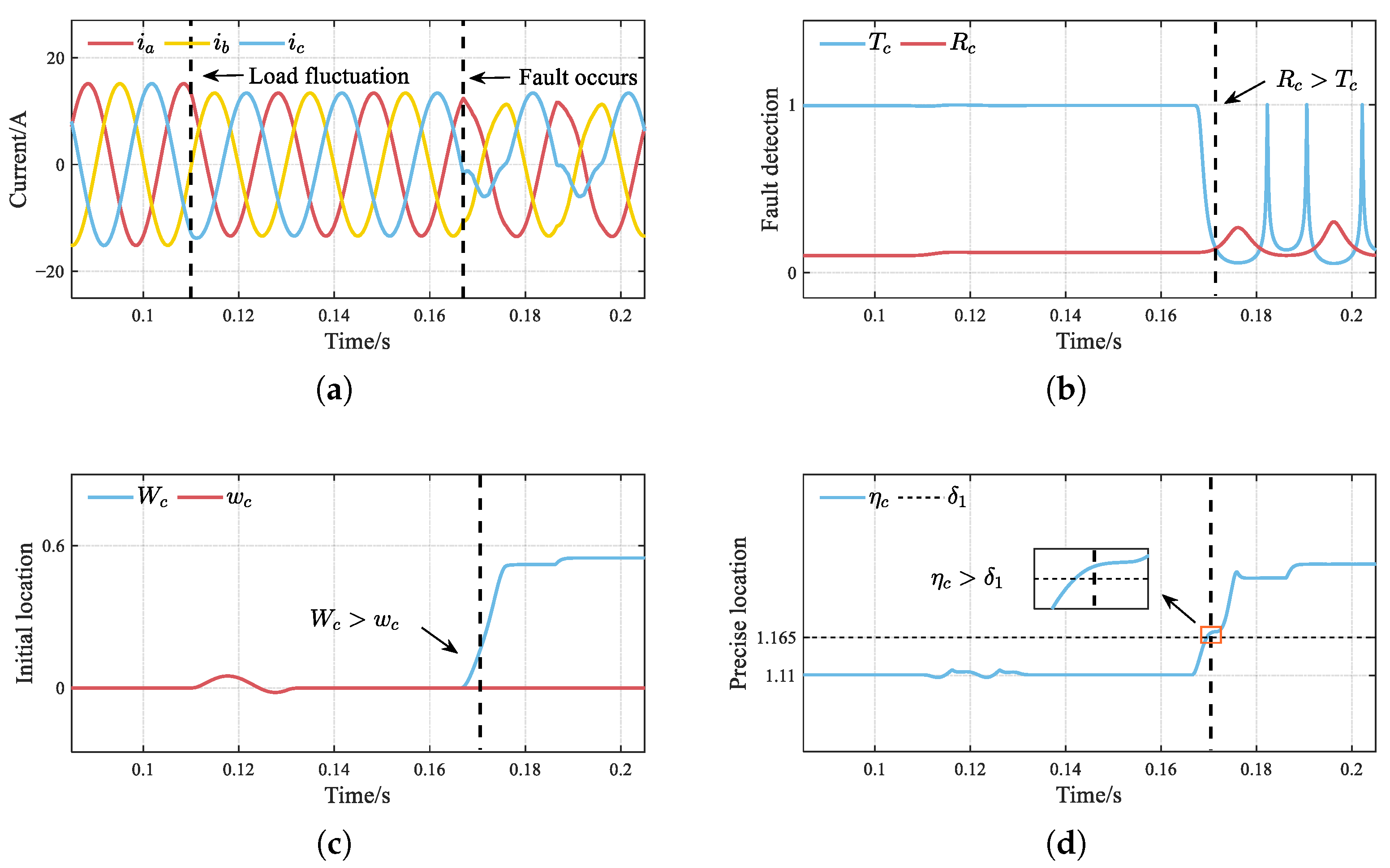
4.3.2. Single-Switch Fault Under Load Fluctuation

Figure 9 illustrates the diagnostic results of switch OC fault under load fluctuation. As shown in the Figure 9, the load resistance increases by $15\%$ at $t=0.11$ s. The detection variable $R_c$ remains consistently below $T_c$, showing no signs of misdiagnosis. When an OC fault occurs in $T_{c4}$ at $t=0.167$ s, both $R_c$ and $T_c$ change, with $R_c$ subsequently exceeding $T_c$. Meanwhile, it is observed that $W_c>w_c$ and ${\eta }_c\ge {\delta }_1$, with all phenomena indicating a fault in $T_{c4}$. The above analysis shows that the proposed method remains reliable without generating false alarms even under load fluctuation, further verifying its robustness.

4.4. Simulation Analysis of Inverter Fault Diagnosis Under Noise Interference

In industrial environments, inverter systems are inherently exposed to persistent stochastic noise during operation. Such noise interacts with fault signature signals through nonlinear coupling mechanisms, substantially complicating the diagnosis of OC faults in power switches. To quantitatively evaluate noise impacts on fault diagnosis, this study simulates practical interference using zero-mean Gaussian white noise with a variance of 3. Taking $T_{b1}$ and $T_{b3}$ faults as representative cases, the figure demonstrates diagnostic outcomes under both ideal and noise-contaminated conditions.

In Figure 10, $T_{b-n}$, $R_{b-n}$, $W_{b-n}$ and ${\eta }_{b-n}$ denote the diagnosis variables under practical operating conditions. As shown in Figure 10a, the adaptive threshold $T_{b-n}$ oscillates around the ideal threshold $T_b$ during normal inverter operation, yet its overall trajectory closely aligns with the ideal curve. Figure 10c reveals that the practical fault location variable ${\eta }_{b-n}$ remains marginally below its ideal counterpart ${\eta }_b$. Furthermore, the discrepancy in fault location time between practical and ideal conditions is merely 0.06 ms.

The proposed fault detection and location method extracts current root mean square (RMS) values to derive current characteristic values and compute location variables. This RMS-based processing approach inherently incorporates statistical smoothing properties, effectively suppressing noise interference and thus ensuring diagnostic accuracy and stability. Consequently, the method demonstrates strong noise robustness, enabling reliable fault diagnosis under practical operating conditions.

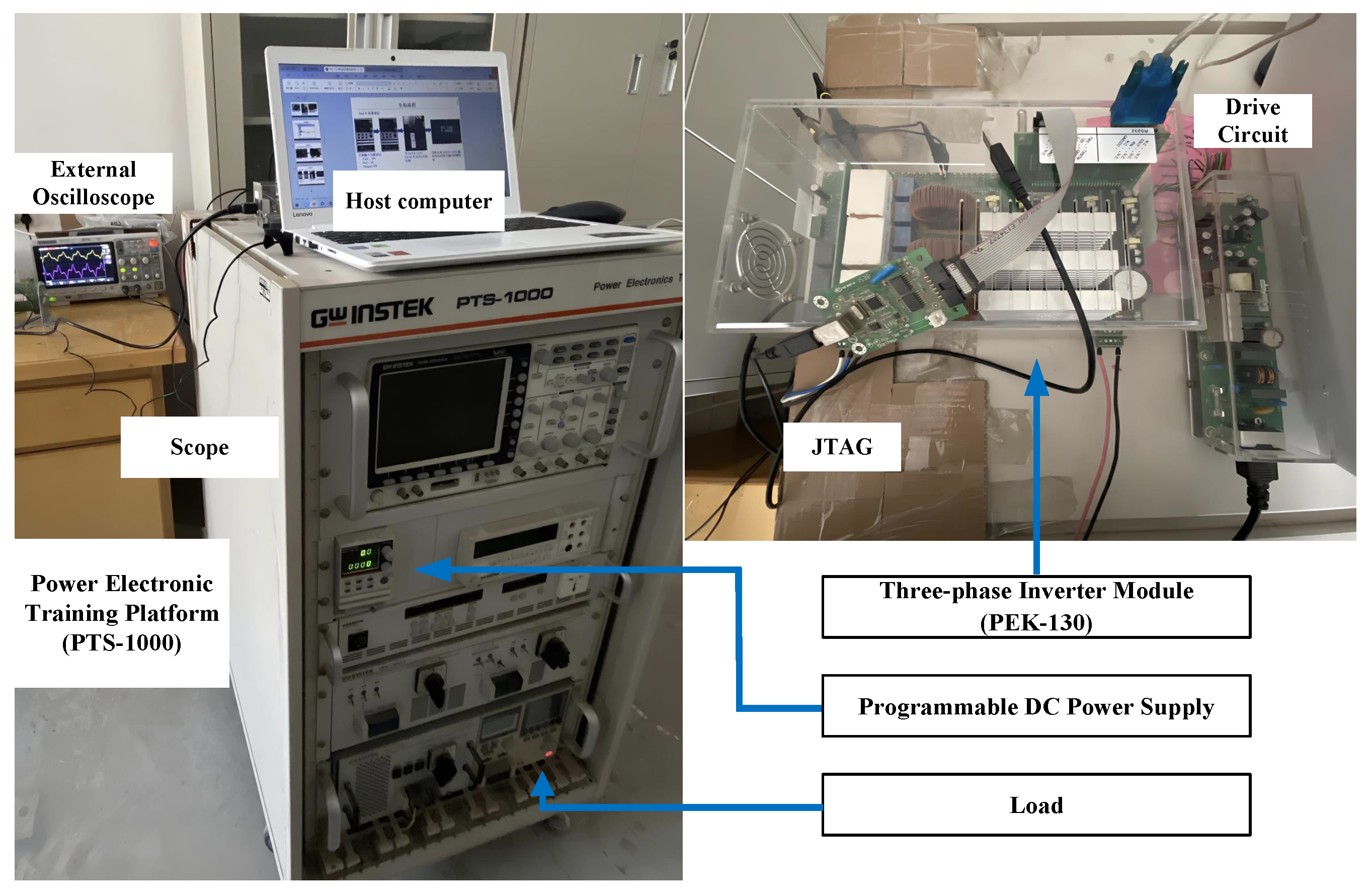
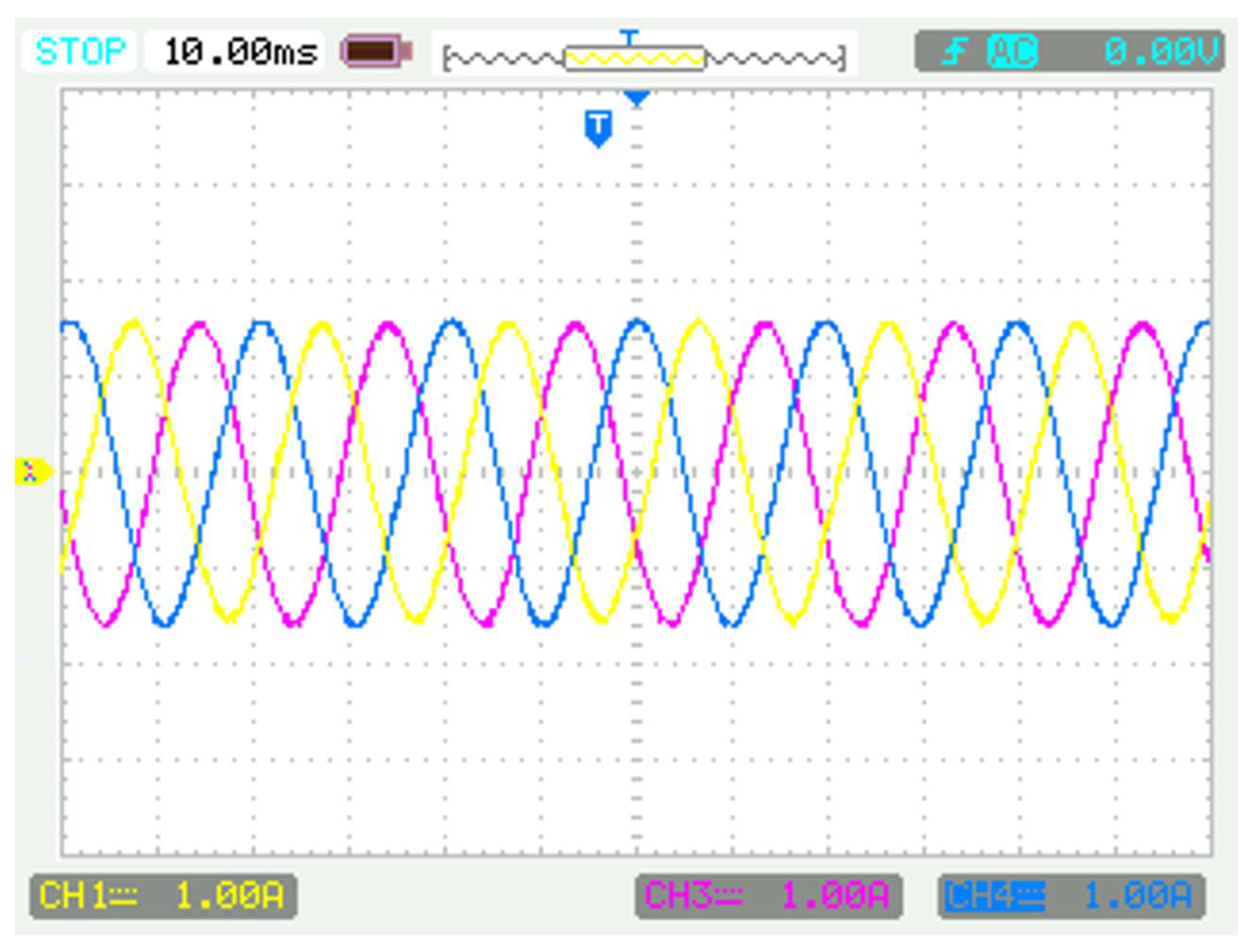
4.5. Experimental Results and Analysis

The inverter system hardware experiment platform is shown in Figure 11. The experimental platform mainly comprises a DC voltage source, a T-type three-level inverter, and a drive module, while the control circuit implemented uses the digital signal processor (TMS320F28335). Specifically, the right image in Figure 11 provides a magnified view of the drive circuit and inverter module in their powered-off state. During the experiment, OC faults in the switches are induced by injecting fault control signals via the PSIM software platform.

Table 4. Experimental platform parameters.

Parameter	Value
DC side voltage ${\mathrm{U}}_{\mathrm{dc}}$	$110\mathrm{V}$
Rated voltage $\mathrm{U}$	$36\mathrm{V}$
Rated output power P	$270\mathrm{W}$
Rated current I	$7.5\mathrm{A}$
Filter inductance L	$4\ast 10^{-3}\mathrm{H}$
Load resistance R	$24\Omega$

presents the relevant parameters of the experimental platform.

Figure 12 shows the three-phase current waveforms measured under normal operating conditions, with the platform powered on and no fault simulation signals applied. The three-phase output currents demonstrate sinusoidal waveform characteristics, maintaining a stable frequency of 50 Hz with consistent ${120}^{\circ }$ phase differences between any two phases. These results are consistent with the simulation outcomes under normal operating conditions.

When conducting fault experiments on the aforementioned platform, the OC fault in the actual inverter is simulated by removing the drive signal associated with the switches. The output current waveforms corresponding to the $T_{a1}$ and $T_{b1}\&T_{b3}$ faults are shown in Figure 13 and Figure 14, respectively, demonstrating consistency with the simulation results illustrated in Figure 5 and Figure 7.

5. Diagnosis Performance Analysis and Comparative Performance Evaluation

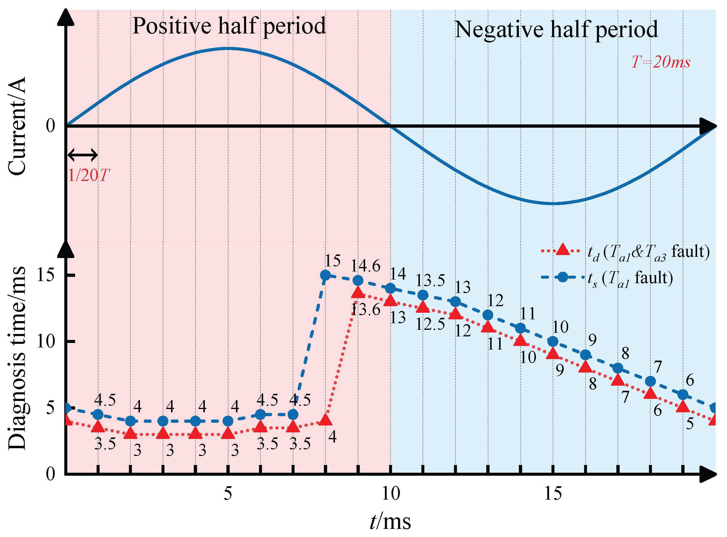
5.1. Diagnosis Time Characteristics Under Different Fault Occurrence Times

To investigate the influence of fault occurrence time on diagnosis speed, Figure 15 illustrates the diagnosis time results at 20 fault instants uniformly distributed within one fundamental period. Here, $t_s$ denotes the diagnosis time for the single-switch fault ($T_{a1}$ OC fault), while $t_d$ represents the diagnosis time for the double-switch fault ($T_{a1}$ and $T_{a3}$ OC fault). Specifically, when the $T_{a1}$ fault occurs in the early segment of the positive half-cycle, rapid diagnosis can usually be achieved. However, as the fault occurrence time shifts towards the latter segment of the positive half-cycle and throughout the entire negative half-cycle, instantaneous fault diagnosis becomes more challenging, and the diagnosis time increases accordingly. This phenomenon primarily arises because $T_{a1}$ OC faults in T-type inverters don’t affect normal operational states during negative half-cycle operation. Consequently, effective diagnosis must be postponed until the subsequent positive half-cycle initiation. Notably, the simultaneous $T_{a1}\&T_{a3}$ OC faults exhibit more distinct signatures, generally enabling shorter detection times compared to single-switch faults.

5.2. Performance Comparisons of Other Methods

To evaluate the performance of the proposed method, this section provides a comparative analysis with existing multilevel fault diagnosis approaches, as detailed in

Table 5. Comparison with previous fault diagnosis methods.

Method	Research Plant	Single/ Multiple Fault	Diagnosis Variable	Hardware/ Calculation Cost	Robustness
[15]	T23L inverter	Multiple	$u_{c1}$, $u_{c2}$, $i_x$	No/High	High
[33]	T23L inverter	Multiple	$u_{xo}$, $i_x$, switching state	Yes/Low	Low
[23]	T23L inverter	Single	$i_x$, $u_{c1}$, $u_{c2}$, $l_x$ and etc.	Yes/Low	High
[19]	T23L inverter	Single	$i_x$, $l_x$ and etc.	No/Low	Low
[18]	T23L inverter	Single	$u_{xo}$	Yes/Low	low
[32]	SPTL inverter	Single	$i_x$, $u_x$	No/Low	High
[31]	NPC inverter	Single	$i_x$	No/Low	High
The proposed method	T23L inverter	Multiple	$i_x$	No/Low	High

. Although [15,33] can achieve multi-switch fault diagnosis for T-type three-level inverters, they exhibit critical limitations. Specifically, Ref. [15] employs a multimodal deep residual network for fault identification. This data-driven approach demands substantial training datasets and computational resources, with experimental measurements indicating an average diagnosis latency of 21 ms. In contrast, as demonstrated in Figure 15, the proposed method achieves faster fault detection, with a maximum detection time not exceeding 15 ms.

Concerning signal requirements, the proposed method requires only three-phase current signals for diagnosis. This contrasts sharply with [19,23,33], which necessitate additional signals such as switching states, pole voltages, and inductance values, thereby increasing diagnostic complexity. Notably, several existing methods depend on voltage signals for fault identification. For instance, Refs. [18,23,33] require voltage signal acquisition, typically implying the need for extra voltage sensors and higher hardware costs. Moreover, Refs. [18,19,33] implement fixed thresholds in their diagnostic processes. These predetermined values demonstrate limited adaptability to dynamic operating conditions and parameter variations, ultimately degrading system robustness.

Comparatively, Refs. [31,32] adopt observer-based methods for multilevel inverter fault diagnosis. While these methods perform well for single-switch faults, they are unable to effectively identify multiple-switch faults. Compared to these approaches, the proposed method not only enables multi-switch fault diagnosis with strong robustness but also demonstrates significant hardware and computational advantages. These are achieved by eliminating the need for additional sensors and reducing calculation cost.

6. Conclusions

This paper proposes an analytical model-based fault diagnosis method for ${\mathrm{T}}^{2}3\mathrm{L}$ inverters, achieving diagnosis of single- and double-switch OC faults within the same phase. First, an improved adaptive sliding mode observer is designed by integrating the hyperbolic tangent function with an adaptive term, which effectively mitigates chattering and improves the precision of phase currents estimation. Then, an adaptive threshold-based fault detection method is proposed to enhance detection robustness and accuracy. Furthermore, fault location variables generated from observed and actual currents enable the precise location of single-switch faults and partial same-phase double-switch faults. The proposed method requires neither additional hardware circuits nor extensive data. Simulation results validate the method’s capability to diagnose single-switch and simultaneous same-phase double-switch faults under complex operating conditions. Building on this, future research could consider more double-switch fault scenarios and design more comprehensive fault diagnosis strategies.

References

1. He, J.; Demerdash, N.A.; Weise, N.; Katebi, R. A fast on-line diagnostic method for open-circuit switch faults in SiC-MOSFET-based T-type multilevel inverters. IEEE Trans. Ind. Appl. 2017, 53, 2948–2958. [Google Scholar] [CrossRef]
2. Mahto, K.K.; Mahato, B.; Chandan, B.; Das, D.; Das, P.; Kumari, S.; Vita, V.; Pavlatos, C.; Fotis, G. A Modified Criss-Cross-Based T-Type MLI with Reduced Power Components. Technologies 2024, 12, 90. [Google Scholar] [CrossRef]
3. Mahto, K.K.; Mahato, B.; Chandan, B.; Das, D.; Das, P.; Fotis, G.; Vita, V.; Mann, M. A new symmetrical source-based DC/AC converter with experimental verification. Electronics 2024, 13, 1975. [Google Scholar] [CrossRef]
4. Chao, K.H.; Chang, L.Y.; Xu, F.Q. Smart fault-tolerant control system based on chaos theory and extension theory for locating faults in a three-level T-type inverter. Appl. Sci. 2019, 9, 3071. [Google Scholar] [CrossRef]
5. Wang, Y.; Li, Y.; Yang, Z.; Cheng, X. An Intelligent Control Strategy for a Highly Reliable Microgrid in Island Mode. Appl. Sci. 2022, 12, 801. [Google Scholar] [CrossRef]
6. He, J.; You, C.C.; Zhang, X.; Li, Z.; Liu, Z. An adaptive dual-loop Lyapunov-based control scheme for a single-phase UPS inverter. IEEE Trans. Power Electron. 2020, 35, 8886–8891. [Google Scholar] [CrossRef]
7. Mahto, K.K.; Pal, P.K.; Das, P.; Mittal, S.; Mahato, B. A new design of multilevel inverter based on T-type symmetrical and asymmetrical DC sources. Trans. Electr. Eng. 2023, 47, 639–657. [Google Scholar] [CrossRef]
8. Zhong, Q.C.; Zhang, X. Impedance-sum stability criterion for power electronic systems with two converters/sources. IEEE Access. 2019, 7, 21254–21265. [Google Scholar] [CrossRef]
9. Gou, B.; Ge, X.; Wang, S.; Feng, X.; Kuo, J.B.; Habetler, T.G. An open-switch fault diagnosis method for single-phase PWM rectifier using a model-based approach in high-speed railway electrical traction drive system. IEEE Trans. Power Electron. 2015, 31, 3816–3826. [Google Scholar] [CrossRef]
10. Zhang, W.; He, Y. A hypothesis method for T-type three-level inverters open-circuit fault diagnosis based on output phase voltage model. IEEE Trans. Power Electron. 2022, 37, 9718–9732. [Google Scholar] [CrossRef]
11. Zhou, Y.; Zhao, J.; Song, Y.; Sun, J.; Fu, H.; Chu, M. A seasonal-trend-decomposition-based voltage-source-inverter open-circuit fault diagnosis method. IEEE Trans. Power Electron. 2022, 37, 15517–15527. [Google Scholar] [CrossRef]
12. Chen, M.; He, Y. Multiple open-circuit fault diagnosis method in NPC rectifiers using fault injection strategy. IEEE Trans. Power Electron. 2022, 37, 8554–8571. [Google Scholar] [CrossRef]
13. Cai, B.; Zhao, Y.; Liu, H.; Xie, M. A data-driven fault diagnosis methodology in three-phase inverters for PMSM drive systems. IEEE Trans. Power Electron. 2016, 32, 5590–5600. [Google Scholar] [CrossRef]
14. Xia, Y.; Xu, Y. A transferrable data-driven method for IGBT open-circuit fault diagnosis in three-phase inverters. IEEE Trans. Power Electron. 2021, 36, 13478–13488. [Google Scholar] [CrossRef]
15. Xing, Z.; He, Y.; Zhang, W. An online multiple open-switch fault diagnosis method for T-type three-level inverters based on multimodal deep residual filter network. IEEE Trans. Ind. Electron. 2022, 70, 10669–10679. [Google Scholar] [CrossRef]
16. Choi, U.M.; Jeong, H.G.; Lee, K.B.; Blaabjerg, F. Method for detecting an open-switch fault in a grid-connected NPC inverter system. IEEE Trans. Power Electron. 2011, 27, 2726–2739. [Google Scholar] [CrossRef]
17. Choi, U.M.; Lee, K.B.; Blaabjerg, F. Diagnosis and tolerant strategy of an open-switch fault for T-type three-level inverter systems. IEEE Trans. Ind. Appl. 2013, 50, 495–508. [Google Scholar] [CrossRef]
18. Liang, Y.; Wang, R.; Hu, B. Single-switch open-circuit diagnosis method based on average voltage vector for three-level T-type inverter. IEEE Trans. Power Electron. 2020, 36, 911–921. [Google Scholar] [CrossRef]
19. Wang, K.; Tang, Y.; Zhang, C.J. Open-circuit fault diagnosis and tolerance strategy applied to four-wire T-type converter systems. IEEE Trans. Power Electron. 2018, 34, 5764–5778. [Google Scholar] [CrossRef]
20. Naseri, F.; Schaltz, E.; Lu, K.; Farjah, E. Real-time open-switch fault diagnosis in automotive permanent magnet synchronous motor drives based on Kalman filter. IET Power Electron. 2020, 13, 2450–2460. [Google Scholar] [CrossRef]
21. Jlassi, I.; Estima, J.O.; El Khil, S.K.; Bellaaj, N.M.; Cardoso, A.J.M. Multiple open-circuit faults diagnosis in back-to-back converters of PMSG drives for wind turbine systems. IEEE Trans. Power Electron. 2014, 30, 2689–2702. [Google Scholar] [CrossRef]
22. Zhou, X.; Sun, J.; Cui, P.; Lu, Y.; Lu, M.; Yu, Y. A fast and robust open-switch fault diagnosis method for variable-speed PMSM system. IEEE Trans. Power Electron. 2020, 36, 2598–2610. [Google Scholar] [CrossRef]
23. Wang, B.; Li, Z.; Bai, Z.; Krein, P.T.; Ma, H. A voltage vector residual estimation method based on current path tracking for T-type inverter open-circuit fault diagnosis. IEEE Trans. Power Electron. 2021, 36, 13460–13477. [Google Scholar] [CrossRef]
24. Huang, S.; Tan, K.K.; Lee, T.H. Fault diagnosis and fault-tolerant control in linear drives using the Kalman filter. IEEE Trans. Power Electron. 2012, 59, 4285–4292. [Google Scholar] [CrossRef]
25. Yong, C.; Zhang, J.; Chen, Z. Current observer-based online open-switch fault diagnosis for voltage-source inverter. ISA Trans. 2020, 99, 445–453. [Google Scholar] [CrossRef]
26. Zhou, H.; Xu, J.; Chen, C.; Tian, X.; Liu, G. Disturbance-observer-based direct torque control of five-phase permanent magnet motor under open-circuit and short-circuit faults. IEEE Trans. Ind. Electron. 2020, 68, 11907–11917. [Google Scholar] [CrossRef]
27. Shao, S.; Wheeler, P.W.; Clare, J.C.; Watson, A.J. Fault detection for modular multilevel converters based on sliding mode observer. IEEE Trans. Power Electron. 2013, 28, 4867–4872. [Google Scholar] [CrossRef]
28. Xu, S.; Zhang, Y.; Hu, Y.; Chai, Y.; Wang, H.; Yang, X.; Ma, M.; Zheng, W.X. Multiple open-switch fault diagnosis for three-phase four-leg inverter under unbalanced loads via interval sliding mode observer. IEEE Trans. Power Electron. 2024, 39, 7607–7619. [Google Scholar] [CrossRef]
29. Zhuo, S.; Xu, L.; Gaillard, A.; Huangfu, Y.; Paire, D.; Gao, F. Robust open-circuit fault diagnosis of multi-phase floating interleaved DC–DC boost converter based on sliding mode observer. IEEE Trans. Transp. Electrif. 2019, 5, 638–649. [Google Scholar] [CrossRef]
30. Sun, T.; Chen, C.; Wang, S.; Zhang, B.; Fu, Y.; Li, J. Inverter open circuit fault diagnosis based on residual performance evaluation. IET Power Electron. 2023, 16, 2560–2576. [Google Scholar] [CrossRef]
31. Xu, S.; Huang, W.; Wang, H.; Zheng, W.; Wang, J.; Chai, Y.; Ma, M. A simultaneous diagnosis method for power switch and current sensor faults in grid-connected three-level NPC inverters. IEEE Trans. Power Electron. 2022, 38, 1104–1118. [Google Scholar] [CrossRef]
32. Xu, S.; Xu, X.; Du, H.; Wang, H.; Chai, Y.; Zheng, W.X.; Chen, H. Comprehensive diagnosis strategy for power switch, grid-side current sensor, DC-link voltage sensor faults in single-phase three-level rectifiers. IEEE Trans. Circuits Syst. I Regul. Pap. 2024, 71, 3343–3356. [Google Scholar] [CrossRef]
33. Wang, B.; Li, Z.; Bai, Z.; Krein, P.T.; Ma, H. Real-time diagnosis of multiple transistor open-circuit faults in a T-type inverter based on finite-state machine model. CPSS Trans. Power Electron. Appl. 2020, 5, 74–85. [Google Scholar] [CrossRef]
Figure 1. T 2 3 L inverter topology.
Applsci 15 06063 g001
Figure 2. Current paths under normal and fault conditions. (a) OC fault in T a 1 . (b) OC fault in T a 4 . (c) OC fault in T a 1 and T a 3 . (d) OC fault in T a 2 . (e) OC fault in T a 3 . (f) OC fault in T a 2 and T a 3 .
Applsci 15 06063 g002
Figure 3. Schematic diagram of the proposed method.
Applsci 15 06063 g003
Figure 4. Conventional switching function versus hyperbolic tangent function curve.
Applsci 15 06063 g004
Figure 5. Simulation results of the T a 1 OC fault. (a) Three-phase currents. (b) Fault detection. (c) Initial location. (d) Precise location.
Applsci 15 06063 g005
Figure 6. Simulation results of the T a 2 OC fault. (a) Three-phase currents. (b) Fault detection. (c) Initial location. (d) Precise location.
Applsci 15 06063 g006
Figure 7. Simulation results of the T b 1 and T b 3 OC fault. (a) Three-phase currents. (b) Fault detection. (c) Initial location. (d) Precise location.
Applsci 15 06063 g007
Figure 8. Simulation results of the T b 2 and T b 4 OC fault under voltage fluctuation. (a) Three-phase currents. (b) Fault detection. (c) Initial location. (d) Precise location.
Applsci 15 06063 g008
Figure 9. Simulation results of the T c 4 OC fault under load fluctuation. (a) Three-phase currents. (b) Fault detection. (c) Initial location. (d) Precise location.
Applsci 15 06063 g009
Figure 10. Comparison of fault diagnosis results under ideal and noisy conditions. (a) Fault detection. (b) Initial location. (c) Precise location.
Applsci 15 06063 g010
Figure 11. Inverter system hardware experiment platform.
Applsci 15 06063 g011
Figure 12. Current waveform of T 2 3 L inverter under normal operation.
Applsci 15 06063 g012
Figure 13. Current waveforms of T 2 3 L inverter under T a 1 OC fault condition.
Applsci 15 06063 g013
Figure 14. Current waveforms of T 2 3 L inverter under T b 1 and T b 3 OC fault condition.
Applsci 15 06063 g014
Figure 15. Diagnosis time of single- and double-switch OC faults.
Applsci 15 06063 g015