
UAV Path Planning Using a State Transition Simulated Annealing Algorithm Based on Integrated Destruction Operators and Backward Learning Strategies

Abstract
1. Introduction
2. UAV Three-Dimensional Path Planning
- The Shortest Path: The total flight distance from the starting point to the endpoint should be minimized.
- Obstacle Avoidance: The flight path must navigate around all obstacles to ensure safety.
- Flight Altitude: The flight path must comply with the specified altitude restrictions.
- Path Smoothness: The trajectory should be as smooth as possible, avoiding sharp turns and steep inclines.
2.1. Path Optimality
2.2. Safety and Feasibility Constraints
3. STASA
3.1. State Transition Operators
- (a)
- Rotation Operator
- (b)
- Translation Operator
- (c)
- Scaling Operator
- (d)
- Axis Transformation Operator
3.2. Update Strategy of the STASA
4. DRSTASA
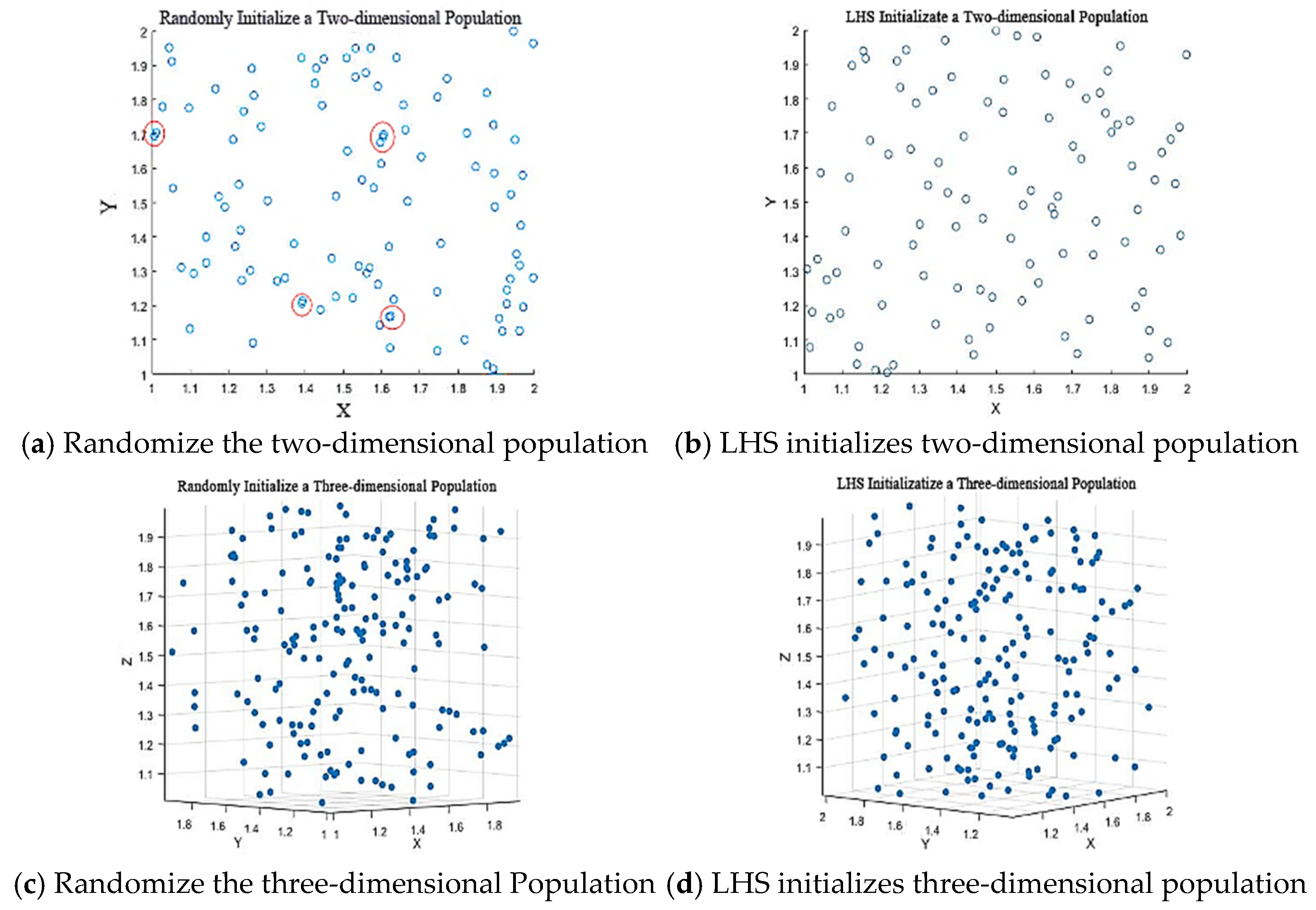
4.1. Population Initialization Based on Latin Hypercube Sampling
4.2. Disruption Operator
4.3. Reverse Learning Strategy
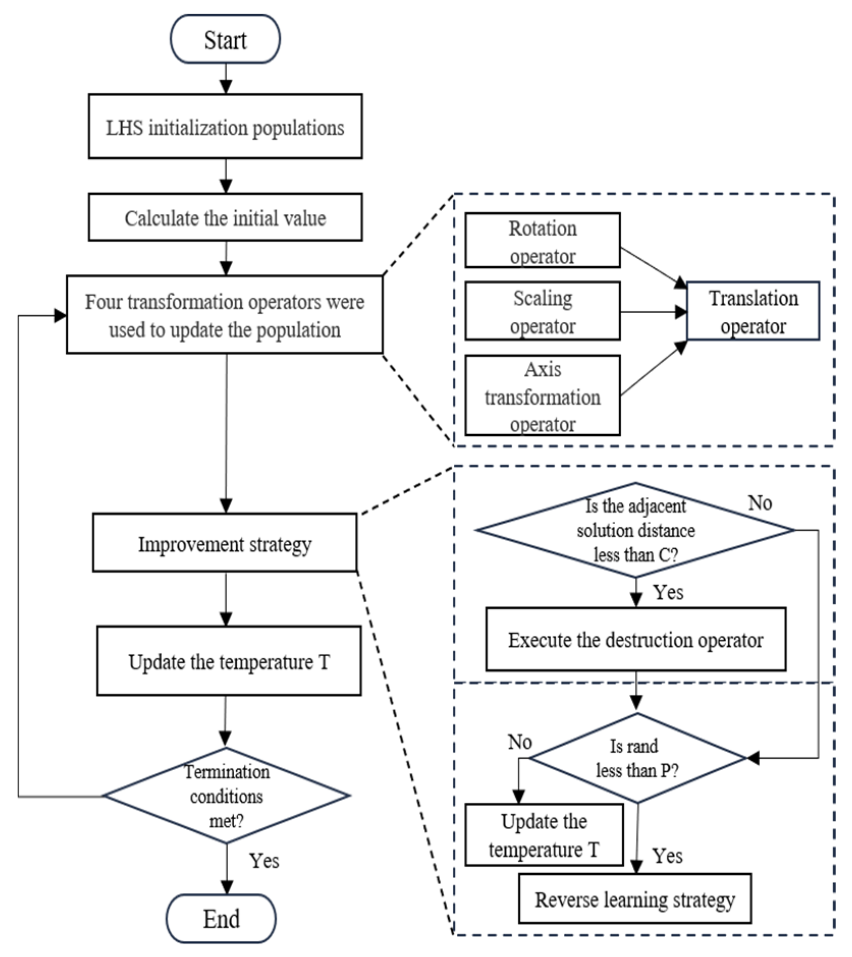
4.4. Basic Process of DRSTASA
| Algorithm 1: The Proposed Algorithm DRSTASA |
| 1: Set the initial parameters 2: LHS generate the initial population u, Evaluate the fitness value: f, the current optimal solution: Best 3: while the set stop temperature value is not reached 4: Update the xk through four transformation operators by Equations (2)–(5) and obtain xk+1. 5: Calculate the fitness value of the current solution and new solution: f(xk), f(xx+1). 6: Update Best and fBest with Metropolis Criteria by Equation (6). 7: Calculate threshold C using Equation (16). 8: Judging by Equation (15), the condition is updated using Equation (17). 9: if rand > p Use Equation (21) to update. 10: T = α*T, k = k + 1 and return to step 4. |
5. Experimental Testing and Analysis
5.1. Benchmark Test Functions
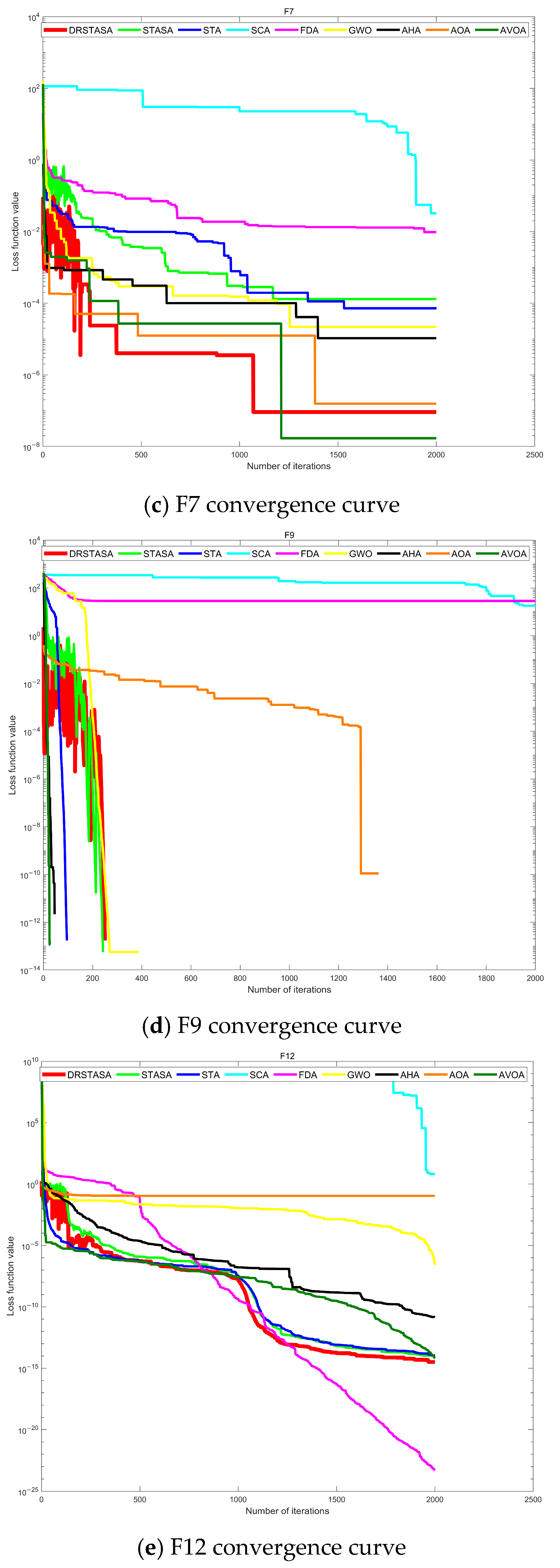
5.1.1. Convergence Analysis
5.1.2. Time Complexity Analysis
5.2. Experimental Results
6. Summary
Author Contributions
Funding
Institutional Review Board Statement
Informed Consent Statement
Data Availability Statement
Conflicts of Interest
References
- Fang, Z.; Savkin, A.V. Strategies for Optimized UAV Surveillance in Various Tasks and Scenarios: A Review. Drones 2024, 8, 193. [Google Scholar] [CrossRef]
- Torrero, L.; Seoli, L.; Molino, A.; Giordan, D.; Manconi, A.; Allasia, P.; Baldo, M. The Use of Micro-UAV to Monitor Active Landslide Scenarios. In Engineering Geology for Society and Territory—Volume 5; Lollino, G., Manconi, A., Guzzetti, F., Culshaw, M., Bobrowsky, P., Luino, F., Eds.; Springer: Cham, Switzerland, 2015. [Google Scholar] [CrossRef]
- Yan, C.; Fu, L.; Zhang, J.; Wang, J. A Comprehensive Survey on UAV Communication Channel Modeling. IEEE Access 2019, 7, 107769–107792. [Google Scholar] [CrossRef]
- Shakhatreh, H.; Sawalmeh, A.H.; Al-Fuqaha, A.; Dou, Z.; Almaita, E.; Khalil, I.; Othman, N.S.; Khreishah, A.; Guizani, M. Unmanned Aerial Vehicles (UAVs): A Survey on Civil Applications and Key Research Challenges. IEEE Access 2019, 7, 48572–48634. [Google Scholar] [CrossRef]
- Hart, P.E.; Nilsson, N.J.; Raphael, B. A Formal Basis for the Heuristic Determination of Minimum Cost Paths. IEEE Trans. Syst. Sci. Cybern. 1968, 4, 100–107. [Google Scholar] [CrossRef]
- Korf, R.E. Depth-First Iterative-Deepening: An Optimal Admissible Tree Search. Artif. Intell. 1985, 27, 97–109. [Google Scholar] [CrossRef]
- Cen, Y.; Song, C.; Xie, N.; Wang, L. Path planning method for mobile robot based on ant colony optimization algorithm. In Proceedings of the 2008 3rd IEEE Conference on Industrial Electronics and Applications, Singapore, 3–5 June 2008; pp. 298–301. [Google Scholar] [CrossRef]
- Qin, Y.-Q.; Sun, D.-B.; Li, N.; Cen, Y.-G. Path planning for mobile robot using the particle swarm optimization with mutation operator. In Proceedings of the 2004 International Conference on Machine Learning and Cybernetics (IEEECat. No. 04EX826), Shanghai, China, 26–29 August 2004; Volume 4, pp. 2473–2478. [Google Scholar] [CrossRef]
- Chen, J.; Ye, F.; Jiang, T. Path planning under obstacle-avoidance constraints based on ant colony optimization algorithm. In Proceedings of the 2017 IEEE 17th International Conference on Communication Technology (ICCT), Chengdu, China, 27–30 October 2017; pp. 1434–1438. [Google Scholar] [CrossRef]
- Guo, L.; Zhao, C.; Li, J.; Yan, Q.; Li, W.; Chen, P. UAV path planning based on improved A * and artificial potential field algorithm. In Proceedings of the 2024 36th Chinese Control and Decision Conference (CCDC), Xi’an, China, 25–27 May 2024; pp. 5471–5476. [Google Scholar] [CrossRef]
- Xiang, H.; Liu, X.; Song, X.; Zhou, W. UAV Path Planning Based on Enhanced PSO-GA. In Artificial Intelligence; Fang, L., Pei, J., Zhai, G., Wang, R., Eds.; CICAI 2023; Lecture Notes in Computer Science; Springer: Singapore, 2024; Volume 14474. [Google Scholar] [CrossRef]
- Li, D.; Yin, W.; Wong, W.E.; Jian, M.; Chau, M. Quality-Oriented Hybrid Path Planning Based on A* and Q-Learning for Unmanned Aerial Vehicle. IEEE Access 2022, 10, 7664–7674. [Google Scholar] [CrossRef]
- Li, B.; Qi, X.; Yu, B.; Liu, L. Trajectory Planning for UAV Based on Improved ACO Algorithm. IEEE Access 2020, 8, 2995–3006. [Google Scholar] [CrossRef]
- Li, H.; Long, T.; Xu, G.; Wang, Y. Coupling-Degree-Based Heuristic Prioritized Planning Method for UAV Swarm Path Generation. In Proceedings of the 2019 Chinese Automation Congress (CAC), Hangzhou, China, 22–24 November 2019; pp. 3636–3641. [Google Scholar] [CrossRef]
- Xie, R.; Meng, Z.; Wang, L.; Li, H.; Wang, K.; Wu, Z. Unmanned Aerial Vehicle Path Planning Algorithm Based on Deep Reinforcement Learning in Large-Scale and Dynamic Environments. IEEE Access 2021, 9, 24884–24900. [Google Scholar] [CrossRef]
- Tan, L.; Zhang, Y.; Huo, J.; Song, S. UAV Path Planning Simulating Driver’s Visual Behavior with RRT algorithm. In Proceedings of the 2019 Chinese Automation Congress (CAC), Hangzhou, China, 22–24 November 2019; pp. 219–223. [Google Scholar] [CrossRef]
- Wang, X.; Pan, J.-S.; Yang, Q.; Kong, L.; Snášel, V.; Chu, S.-C. Modified Mayfly Algorithm for UAV Path Planning. Drones 2022, 6, 134. [Google Scholar] [CrossRef]
- Tian, J.; Wang, Y.; Yuan, D. An Unmanned Aerial Vehicle Path Planning Method Based on the Elastic Rope Algorithm. In Proceedings of the 2019 IEEE 10th International Conference on Mechanical and Aerospace Engineering (ICMAE), Brussels, Belgium, 22–25 July 2019; pp. 137–141. [Google Scholar] [CrossRef]
- Cui, X.; Wang, Y.; Yang, S.; Liu, H.; Mou, C. UAV path planning method for data collection of fixed-point equipment in complex forest environment. Front. Neurorobot. 2022, 16, 1105177. [Google Scholar] [CrossRef]
- Yu, X.; Li, C.; Zhou, J. A constrained differential evolution algorithm to solve UAV path planning in disaster scenarios. Knowl.-Based Syst. 2020, 204, 106209. [Google Scholar] [CrossRef]
- Zhang, X.; Xia, S.; Li, X. Quantum Behavior-Based Enhanced Fruit Fly Optimization Algorithm with Application to UAV Path Planning. Int. J. Comput. Intell. Syst. 2020, 13, 1315–1331. [Google Scholar] [CrossRef]
- Qu, C.; Gai, W.; Zhang, J.; Zhong, M. A novel hybrid grey wolf optimizer algorithm for unmanned aerial vehicle (UAV) path planning. Knowl.-Based Syst. 2020, 194, 105530. [Google Scholar] [CrossRef]
- Chen, Y.; Yu, Q.; Han, D.; Jiang, H. UAV path planning: Integration of grey wolf algorithm and artificial potential field. Concurr. Comput. Pract. Exp. 2024, 36, e8120. [Google Scholar] [CrossRef]
- Han, X.; Dong, Y.; Yue, L.; Xu, Q. State Transition Simulated Annealing Algorithm for Discrete-Continuous Optimization Problems. IEEE Access 2019, 7, 44391–44403. [Google Scholar] [CrossRef]
- Zhou, X.; Yang, C.; Gui, W. State Transition Algorithm. J. Ind. Manag. Optim. 2012, 8, 1039–1056. [Google Scholar] [CrossRef]
- Aarts, E.H.L. Simulated Annealing: Theory and Applications; Springer Nature: Dordrecht, The Netherlands, 1987. [Google Scholar]
- Chu, J.; Dong, Y.; Han, X.; Xie, J.; Xu, X.; Xie, G. Short-term prediction of urban PM2. 5 based on a hybrid modified variational mode decomposition and support vector regression model. Environ. Sci. Pollut. Res. 2021, 28, 56–72. [Google Scholar] [CrossRef]
- Shen, Y.; Dong, Y.; Han, X.; Wu, J.; Xue, K.; Jin, M.; Xie, G.; Xu, X. Prediction model for methanation reaction conditions based on a state transition simulated annealing algorithm optimized extreme learning machine. Int. J. Hydrog. Energy 2023, 48, 24560–24573. [Google Scholar] [CrossRef]
- Alhijawi, B.; Awajan, A. Genetic algorithms: Theory, genetic operators, solutions, and applications. Evol. Intel. 2024, 17, 1245–1256. [Google Scholar] [CrossRef]
- Mirjalili, S.; Mirjalili, S.M.; Lewis, A. Grey Wolf Optimizer. Adv. Eng. Softw. 2014, 69, 46–61, ISSN 0965-9978. [Google Scholar] [CrossRef]
- Phung, M.D.; Ha, Q.P. Safety-enhanced UAV path planning with spherical vector-based particle swarm optimization. Appl. Soft Comput. 2021, 107, 107376. [Google Scholar] [CrossRef]
- Dige, N.; Diwekar, U. Efficient sampling algorithm for large-scale optimization under uncertainty problems. Comput. Chem. Eng. 2018, 115, 431–454. [Google Scholar] [CrossRef]
- Rashedi, E.; Nezamabadi-pour, H.; Saryazdi, S. GSA: A Gravitational Search Algorithm. Inf. Sci. 2009, 179, 2232–2248. [Google Scholar] [CrossRef]
- Sarafrazi, S.; Nezamabadi-pour, H.; Saryazdi, S. Disruption: A new operator in gravitational search algorithm. Sci. Iran. 2011, 18, 539–548. [Google Scholar] [CrossRef]
- Liu, H.; Ding, G.; Wang, B. Bare-bones particle swarm optimization with disruption operator. Appl. Math. Comput. 2014, 238, 106–122. [Google Scholar] [CrossRef]
- Shekhawat, S.; Saxena, A. Development and applications of an intelligent crow search algorithm based on opposition based learning. ISA Trans. 2020, 99, 210–230. [Google Scholar] [CrossRef]
- Gupta, S.; Deep, K. A hybrid self-adaptive sine cosine algorithm with opposition based learning. Expert Syst. Appl. 2019, 119, 210–230. [Google Scholar] [CrossRef]


| Algorithm | Name and Year of Publication | Parameter Settings |
|---|---|---|
| STA | State Transition Algorithm/2012 | SE = 50, T = 1010, beta = 1, gamma = 1, delta = 1; |
| STASA | State Transition Simulated Annealing Algorithm/2019 | SE = 50, T = 1010, beta = 1, gamma = 1, delta = 1, a = 0.93; |
| AOA | Arithmetic Optimization Algorithm/2021 | Max_iteration = 2000, PopSize = 50; |
| SCA | Sine Cosine Algorithm/2016 | Pop_size = 50, Max_iter = 2000, a = 2; |
| AHA | Artificial Hummingbird Algorithm/2021 | Max_iteration = 2000, Pop_size = 50; |
| FDA | Flow Direction Algorithm/2021 | alpha = 50, beta = 1, Max_iteration = 2000; |
| AVOA | African Vultures Optimization Algorithm/2021 | Pop_size = 50, Max_iter = 2000, p1 = 0.6, p2 = 0.4, p3 = 0.6, alpha = 0.8, betha = 0.2, gamma = 2.5; |
| GWO | Grey Wolf Optimizer Algorithm/2014 | SearchAgents_no = 50, Max_iteration = 2000;; |
| ASTASA | Adaptive State Transition Simulated Annealing Algorithm/2023 | SE = 50,Tp = 10, a1 = a2 = 0.5, T = 1010, a = 0.93, Ω = {0, 0.5, 0.1, 0.1, 1 × 10⁻³, 1 × 10⁻⁶, 1 × 10⁻⁹}; |
| Function | Value Range | Best |
|---|---|---|
| [−100, 100] | 0 | |
| [−10, 10] | 0 | |
| [−100, 100] | 0 | |
| [−100, 100] | 0 | |
| [−30, 30] | 0 | |
| [−100, 100] | 0 | |
| [−1.28, 1.28] | 0 |
| Function | Dimension | Value Range | Best |
|---|---|---|---|
| d | [−500, 500] | ||
| d | [−5.12, 5.12] | 0 | |
| d | [−32, 32] | 0 | |
| d | [−600, 600] | 0 | |
| d | [−50, 50] | 0 | |
| d | [−50, 50] | 0 | |
| 2 | [−65.53, 65.53] | 1 | |
| 4 | [−5, 5] | 0.00030 | |
| 2 | [−5, 5] | −1.0316 | |
| 2 | [−5, 5] | 0.398 | |
| 2 | [−2, 2] | 3 | |
| 3 | [1, 3] | −3.86 | |
| 6 | [0, 1] | −3.32 | |
| 4 | [0, 10] | −10.1532 | |
| 4 | [0, 10] | −10.4028 | |
| 4 | [0, 10] | −10.5363 |
| DSTASA | STASA | SCA | AOA | STA | AHA | FDA | AVOA | GWO | ASTASA | ||
|---|---|---|---|---|---|---|---|---|---|---|---|
| F1 | min | 0 | 0 | 2.23826 × 10⁻⁵ | 0 | 0 | 0 | 2.49859 × 10⁻²⁷ | 0 | 6.545097 × 10−127 | 0 |
| mean | 0 | 0 | 2.22950 × 10⁻⁵ | 0 | 0 | 0 | 8.20562 × 10⁻²⁵ | 0 | 1.11579 × 10−121 | 0 | |
| std | 0 | 0 | 4.41827 × 10⁻⁵ | 0 | 0 | 0 | 1.69896 × 10⁻²⁴ | 0 | 2.81725 × 10−121 | 0 | |
| R | 0 | 1 | 0 | 0 | 0 | 1 | 0 | 1 | 0 | ||
| F2 | min | 0 | 0 | 1.36292 × 10⁻⁸ | 0 | 0 | 0 | 5.12704 × 10⁻²⁰ | 0 | 3.19172 × 10−72 | 2.73 × 10−298 |
| mean | 0 | 0 | 2.18929 × 10⁻³ | 0 | 0 | 9.75350 × 10−305 | 5.80501 × 10⁻¹⁹ | 0 | 9.43916 × 10−71 | 5.78 × 10−285 | |
| std | 0 | 0 | 5.07143 × 10⁻³ | 0 | 0 | 0 | 9.87080 × 10⁻¹⁹ | 0 | 1.50523 × 10−70 | 0 | |
| R | 0 | 1 | 0 | 0 | 1 | 1 | 0 | 1 | 1 | ||
| F3 | min | 0 | 0 | 5.34185 × 10⁻² | 0 | 1.67556 × 10−165 | 0 | 8.44382 × 10⁻⁵ | 0 | 1.66451 × 10−40 | 2.45 × 10−39 |
| mean | 0 | 6.39864 × 10⁻¹⁰ | 1.64976 × 10² | 0 | 2.11171 × 10⁻¹⁰ | 0 | 1.19773 × 10⁻³ | 0 | 2.20731 × 10⁻³² | 8.25 × 10⁻¹³ | |
| std | 0 | 2.32239 × 10⁻⁹ | 4.05739 × 10² | 0 | 4.67669 × 10⁻¹⁰ | 0 | 1.54680 × 10⁻³ | 0 | 8.16378 × 10⁻³² | 2.68 × 10⁻¹² | |
| R | 1 | 1 | 0 | 1 | 0 | 1 | 0 | 1 | 1 | ||
| F4 | min | 0 | 1.40860 × 10−320 | 0.012679128 | 0 | 2.75719 × 10−294 | 2.76011 × 10−291 | 5.858143094 | 0 | 9.51328 × 10⁻³³ | 5.47 × 10−125 |
| mean | 0 | 2.78906 × 10−305 | 3.541937518 | 4.11638 × 10⁻³ | 3.20126 × 10−252 | 3.20126 × 10−252 | 11.58330534 | 0 | 9.71144 × 10⁻³⁰ | 9.77 × 10⁻¹⁰ | |
| std | 0 | 0 | 5.806930164 | 1.25609 × 10⁻³ | 0 | 0 | 2.472639669 | 0 | 2.56898 × 10⁻²⁹ | 3.66 × 10⁻⁹ | |
| R | - | 1 | 1 | 1 | 1 | 1 | 1 | 0 | 1 | 1 | |
| F5 | min | 1.68646 × 10⁻⁸ | 21.08270450 | 39.98909064 | 25.80156310 | 20.72509086 | 23.25891369 | 9.56426 × 10⁻⁵ | 4.08905 × 10⁻⁸ | 25.19991104 | 19.22748051 |
| mean | 17.8889 | 21.66482354 | 415349.1403 | 27.18829167 | 23.30892552 | 23.76828972 | 13.80940547 | 7.48172 × 10⁻⁷ | 26.33910544 | 19.60826434 | |
| std | 8.1378 | 0.273833566 | 7.79634 × 10⁵ | 0.684053143 | 9.635097572 | 0.307795962 | 16.79242368 | 8.34461 × 10⁻⁷ | 0.724028375 | 0.185495286 | |
| R | - | 1 | 1 | 1 | 1 | 1 | 1 | 1 | 1 | 1 | |
| F6 | min | 6.39082 × 10⁻¹⁴ | 6.56884 × 10⁻¹⁴ | 5.261395082 | 1.308848294 | 4.734708 × 10⁻¹⁴ | 2.29367 × 10⁻¹⁰ | 4.61674 × 10⁻²⁸ | 3.31762 × 10⁻¹² | 0.248994178 | 8.02 × 10⁻²² |
| mean | 1.13264 × 10⁻¹³ | 1.10163 × 10⁻¹³ | 149.8606905 | 1.815537219 | 9.077552 × 10⁻¹⁴ | 2.91864 × 10⁻⁸ | 3.53723 × 10⁻²⁵ | 2.03156 × 10⁻¹¹ | 0.707049993 | 4.52 × 10⁻¹⁹ | |
| std | 3.30438 × 10⁻¹⁴ | 3.42395 × 10⁻¹⁴ | 595.3156887 | 0.243828926 | 3.397547 × 10⁻¹⁴ | 6.42005 × 10⁻⁸ | 1.20000 × 10⁻²⁴ | 1.36005 × 10⁻¹¹ | 0.352646793 | 9.58 × 10⁻¹⁹ | |
| R | - | 1 | 1 | 1 | −1 | 1 | −1 | 1 | 1 | −1 | |
| F7 | min | 9.09943 × 10⁻⁸ | 5.78305 × 10⁻⁴ | 0.040713560 | 3.95305 × 10⁻⁷ | 4.29126 × 10⁻⁵ | 2.52943 × 10⁻⁶ | 9.43934 × 10⁻³ | 1.50881 × 10⁻⁶ | 3.73270 × 10⁻⁵ | 0.000105144 |
| mean | 1.73036 × 10⁻⁶ | 6.17465 × 10⁻⁴ | 0.801106982 | 5.62328 × 10⁻⁶ | 5.52640 × 10⁻⁴ | 2.64510 × 10⁻⁵ | 9.43934 × 10⁻³ | 3.52845 × 10⁻⁵ | 3.39785 × 10⁻⁴ | 0.010289159 | |
| std | 1.54743 × 10⁻⁶ | 6.61753 × 10⁻⁴ | 1.605338652 | 4.83192 × 10⁻⁶ | 4.07464 × 10⁻⁴ | 2.16516 × 10⁻⁵ | 1.01640 × 10⁻² | 3.79440 × 10⁻⁵ | 1.85178 × 10⁻⁴ | 0.008127468 | |
| R | - | 1 | 1 | 1 | 1 | 1 | 1 | 1 | 1 | 1 | |
| F8 | min | −12,569.4866 | −12,569.4866 | −5476.55146 | −8318.39435 | −12,569.4866 | −12,569.4865 | −10,316.1050 | −12,569.4866 | −7925.33057 | −12,569.4866 |
| mean | −12,569.4866 | −12,464.6926 | −4321.69164 | −7716.85829 | −12,569.4866 | −12,541.8054 | −8984.9918 | −12,538.5609 | −6031.63602 | −12,290.9614 | |
| std | 3.46119 × 10⁻¹² | 197.5076886 | 297.4265754 | 315.7564352 | 6.47089 × 10⁻¹² | 105.2953070 | 677.695949 | 80.25593103 | 709.6064865 | 291.5008075 | |
| R | - | 1 | 1 | 1 | 1 | 1 | 1 | 1 | 1 | 1 | |
| F9 | min | 0 | 0 | 6.728109115 | 0 | 0 | 0 | 27.85883344 | 0 | 0 | 0 |
| mean | 0 | 0 | 82.76259996 | 0 | 0 | 0 | 51.67162761 | 0 | 0.1419434548 | 0 | |
| std | 0 | 0 | 51.50064571 | 0 | 0 | 0 | 14.98471084 | 0 | 0.7774563208 | 0 | |
| R | - | 0 | 1 | 0 | 0 | 0 | 1 | 0 | 1 | 0 | |
| F10 | min | 8.88178 × 10⁻¹⁶ | 8.88178 × 10⁻¹⁶ | 0.215951010 | 8.88178 × 10⁻¹⁶ | 4.440892 × 10⁻¹⁵ | 8.88178 × 10⁻¹⁶ | 2.120053361 | 8.88178 ×10⁻¹⁶ | 7.99360 × 10⁻¹⁵ | 8.88178 × 10⁻¹⁶ |
| mean | 8.88178 × 10⁻¹⁶ | 8.88178 × 10⁻¹⁶ | 17.68353321 | 8.88178 × 10⁻¹⁶ | 4.440892 × 10⁻¹⁵ | 8.88178 × 10⁻¹⁶ | 3.522161581 | 8.88178 × 10⁻¹⁶ | 8.82257 × 10⁻¹⁵ | 8.88178 × 10⁻¹⁶ | |
| std | 0 | 0 | 5.866102058 | 0 | 0 | 0 | 1.081526236 | 0 | 2.01908 × 10⁻¹⁵ | 0 | |
| R | - | 0 | 1 | 0 | 1 | 0 | 1 | 0 | 1 | 0 | |
| F11 | min | 0 | 0 | 0.291675643 | 0 | 0 | 0 | 0 | 0 | 0 | 0 |
| mean | 0 | 0 | 2.078403009 | 0.031828867 | 0 | 0 | 0.098300745 | 0 | 6.82138 × 10⁻⁴ | 0 | |
| std | 0 | 0 | 2.803796744 | 0.031945879 | 0 | 0 | 0.028645710 | 0 | 0.002679238 | 0 | |
| R | - | 0 | 1 | 1 | 0 | 0 | 1 | 0 | 1 | 0 | |
| F12 | min | 3.21421 × 10⁻¹⁵ | 1.47667 × 10⁻¹⁵ | 0.847785404 | 0.080714235 | 2.36383 × 10⁻¹⁵ | 1.88023 × 10⁻¹¹ | 6.24752 × 10⁻²⁴ | 2.99681 × 10⁻¹³ | 0.011988789 | 7.06 × 10⁻²⁴ |
| mean | 5.81410 × 10⁻¹⁵ | 5.67626 × 10⁻¹⁵ | 3.49168 × 10⁷ | 0.123240492 | 5.75915 × 10⁻¹⁵ | 1.25750 × 10⁻⁹ | 0.411870057 | 1.38250 × 10⁻¹² | 0.030024875 | 1.07 × 10⁻²⁰ | |
| std | 1.77067 × 10⁻¹⁵ | 8.06953 × 10⁻¹⁵ | 1.18813 × 10⁸ | 0.043268406 | 1.39051 × 10⁻¹⁵ | 4.33242 × 10⁻⁹ | 0.545587377 | 1.04906 × 10⁻¹² | 0.011955839 | 2.70 × 10⁻²⁰ | |
| R | - | -1 | 1 | 1 | -1 | 1 | -1 | 1 | 1 | -1 | |
| F13 | min | 3.18192 × 10⁻¹⁴ | 3.67286 × 10⁻¹⁴ | 7.123647255 | 2.408009950 | 4.22109 × 10⁻¹⁴ | 3.76686 × 10⁻⁹ | 3.37417 × 10⁻²⁴ | 1.61800 × 10⁻¹¹ | 0.100047883 | 1.96 × 10⁻²² |
| mean | 7.94253 × 10⁻¹⁴ | 7.95419 × 10⁻¹⁴ | 5.48897 × 10⁷ | 2.696393591 | 8.33771 × 10⁻¹⁴ | 0.305832578 | 0.013540213 | 1.51531 × 10⁻¹⁰ | 0.445347041 | 0.045889875 | |
| std | 2.43030 × 10⁻¹⁴ | 1.46694 × 10⁻¹³ | 1.27678 × 10⁸ | 0.143791836 | 2.36018 × 10⁻¹⁴ | 0.235506620 | 0.028354695 | 1.14064 × 10⁻¹⁰ | 0.183978024 | 0.102558824 | |
| R | - | 1 | 1 | 1 | 1 | 1 | −1 | 1 | 1 | −1 | |
| F14 | min | 0.998003837 | 2.982105156 | 0.998003837 | 0.998003837 | 0.998003837 | 0.998003837 | 0.998003837 | 0.998003837 | 0.998003837 | 0.998003838 |
| mean | 4.499754429 | 5.438523655 | 0.998037194 | 7.770896036 | 4.779597260 | 0.998003837 | 0.998003837 | 0.998003837 | 3.678543020 | 5.692655933 | |
| std | 5.440455117 | 4.165793216 | 0.000061096 | 4.433286361 | 4.522047715 | 0 | 0 | 1.93398 × 10⁻¹⁶ | 3.713426710 | 4.557993224 | |
| R | - | 1 | −1 | 1 | 1 | −1 | −1 | −1 | −1 | 1 | |
| F15 | min | 0.000307485 | 0.000307485 | 0.000357134 | 0.000320376 | 0.000307485 | 0.000307485 | 0.0003.07485 | 0.000307486 | 0.000307486 | 0.000307486 |
| mean | 0.000307485 | 0.000439713 | 0.000884466 | 0.005313377 | 0.000379456 | 0.000307485 | 5.51669 × 10⁻⁴ | 0.000307504 | 0.007661302 | 0.000514668 | |
| std | 3.62847 × 10⁻¹⁴ | 0.000315020 | 0.000308607 | 0.012872782 | 0.000237006 | 1.66935 × 10⁻¹³ | 4.11854 × 10⁻⁴ | 5.88603 × 10⁻⁸ | 0.009830023 | 0.00039831 | |
| R | - | 1 | 1 | 1 | 1 | 1 | 1 | 1 | 1 | 1 | |
| F16 | min | −1.03162845 | −1.03162845 | −1.03162807 | −1.03162845 | −1.03162845 | −1.03162845 | −1.03162845 | −1.03162845 | −1.03162845 | −1.03162845 |
| mean | −1.03162845 | −1.03162845 | −1.03160669 | −1.03162842 | −1.03162845 | −1.03162845 | −1.03162845 | −1.03162845 | −1.03162845 | −1.03162845 | |
| std | 4.38309 × 10⁻¹⁶ | 6.15734 × 10⁻¹⁶ | 2.45274 × 10⁻⁵ | 2.16194 × 10⁻⁸ | 4.75518 × 10⁻¹⁶ | 0.397887357 | 6.77521 × 10⁻¹⁶ | 5.13342 × 10⁻¹⁶ | 1.12689 × 10⁻⁹ | 4.52 × 10⁻¹⁶ | |
| R | - | 1 | −1 | 1 | 1 | 1 | −1 | 1 | 1 | 1 | |
| F17 | min | 0.397887357 | 0.397887357 | 0.397895813 | 0.397887357 | 0.397887357 | 0.397887357 | 0.397887357 | 0.397887357 | 0.397887358 | 0.397887358 |
| mean | 0.397887357 | 0.397887357 | 0.398317876 | 0.397887373 | 0.397887357 | 0.397887357 | 0.397887357 | 0.397887357 | 0.397887418 | 0.397887358 | |
| std | 0 | 0 | 9.39071 × 10⁻¹³ | 1.39785 × 10⁻⁸ | 0 | 0 | 0 | 0 | 7.21333 × 10⁻⁸ | 0 | |
| R | - | 0 | 1 | 1 | 0 | 0 | 0 | 0 | 1 | 1 | |
| F18 | min | 3 | 3 | 3 | 3 | 3 | 3 | 3 | 3 | 3 | 3 |
| mean | 3 | 3 | 3 | 24.22626137 | 3 | 3 | 3 | 3 | 8.400002379 | 3 | |
| std | 1.90209 × 10⁻¹⁴ | 2.00653 × 10⁻¹⁴ | 1.40481 × 10⁻⁵ | 29.41664391 | 2.48436 × 10⁻¹⁴ | 1.27488× 10⁻¹⁵ | 2.01660 × 10⁻¹⁵ | 6.61248 × 10⁻⁸ | 20.55035868 | 4.95 × 10⁻¹⁶ | |
| R | - | 1 | 1 | 1 | 1 | −1 | −1 | 1 | 1 | 1 | |
| F19 | min | −3.86278214 | −3.86278214 | −3.86151460 | −3.86111628 | −3.86278214 | −3.86278214 | −3.86278214 | −3.86278214 | −3.86278214 | −3.86278215 |
| mean | −3.86278214 | −3.86278214 | −3.85507954 | −3.85687242 | −3.86278214 | −3.86278214 | −3.86278214 | −3.86278214 | −3.86184716 | −3.86278215 | |
| std | 1.45290 × 10⁻¹⁴ | 3.78218 × 10⁻¹⁴ | 0.001985413 | 2.89580 × 10⁻³ | 5.20156 × 10⁻¹⁴ | 2.71008 × 10⁻¹⁵ | 2.71008 × 10⁻¹⁵ | 2.14885 × 10⁻¹⁵ | 0.002259703 | 2.31 × 10⁻¹⁵ | |
| R | - | 1 | 1 | 1 | 1 | 1 | 1 | 1 | 1 | 1 | |
| F20 | min | −3.32199517 | −3.32199517 | −3.15647379 | −3.25828015 | −3.32199517 | −3.32199517 | −3.32199517 | −3.32199517 | −3.321994517 | −3.32199517 |
| mean | −3.22688067 | −3.22291757 | −2.98017193 | −3.17153577 | −3.26254861 | −3.32199517 | −3.30614275 | −3.28632723 | −3.26180981 | −3.24669620 | |
| std | 0.048370251 | 0.045066321 | 0.166303220 | 0.035538315 | 0.060462814 | 1.34243 × 10⁻¹⁵ | 0.041106809 | 0.055415085 | 0.068484869 | 0.058273385 | |
| R | −1 | 1 | 1 | 1 | −1 | 1 | 1 | 1 | 1 | ||
| F21 | min | −10.1531996 | −5.05519772 | −5.71194546 | −8.30382836 | −10.15319967 | −10.1531996 | −10.1531996 | −10.1531996 | −10.1531868 | −10.1531997 |
| mean | −5.90486472 | −5.05519772 | −3.33330583 | −4.75221370 | −7.032031215 | −9.90418836 | −9.90418836 | −10.1531996 | −9.47487572 | −8.04555502 | |
| std | 1.932392652 | 6.53716 × 10⁻¹⁵ | 1.649205881 | 1.248257971 | 2.6280332184 | 1.363891112 | 1.363891112 | 4.51078 × 10⁻¹⁵ | 1.758656268 | 2.659975707 | |
| R | - | 1 | 1 | 1 | −1 | −1 | −1 | −1 | −1 | 1 | |
| F22 | min | −10.4029405 | −5.08767182 | −5.86881454 | −9.03871310 | −10.40294056 | −10.4029405 | −10.4029405 | −10.4029405 | −10.4029243 | −10.4029406 |
| mean | −6.32790119 | −5.08767182 | −3.47931164 | −5.64706181 | −8.915907821 | −10.4029405 | −9.12752888 | −10.4029405 | −10.4028323 | −9.1468558 | |
| std | 2.286538610 | 4.49568 × 10⁻¹⁵ | 1.754731464 | 1.594763783 | 2.5417202149 | 1.58195 × 10⁻¹⁵ | 2.622221264 | 1.27754 × 10⁻¹⁵ | 7.26464 × 10⁻⁵ | 2.37780875 | |
| R | - | 1 | 1 | 1 | −1 | −1 | −1 | −1 | −1 | 1 | |
| F23 | min | −10.5364098 | −5.12848078 | −5.69960702 | −8.60971414 | −10.53640981 | −10.5364098 | −10.5364098 | −10.5364098 | −10.5364073 | −10.5364098 |
| mean | −6.39033089 | −5.30874508 | −3.84238656 | −5.16251028 | −9.815352612 | −10.5364098 | −9.95408731 | −10.5364098 | −10.5363015 | −9.1018401 | |
| std | 2.326399497 | 0.987348239 | 1.165562137 | 1.850734616 | 1.8697693093 | 1.89490 × 10⁻¹⁵ | 1.788022077 | 3.55271 × 10⁻¹⁵ | 5.50112 × 10⁻⁵ | 2.41893659 | |
| R | - | 1 | 1 | 1 | −1 | −1 | −1 | −1 | −1 | −1 | |
| - | 13 | 19 | 18 | 8 | 5 | 4 | 7 | 15 | 11 |
| Engineering Issues | Attribute |
|---|---|
| 1. Compression spring design | 3 variables, 4 constraints |
| 2. I-beam design | 4 variables, 2 constraints |
| 3. Welded Beam Design | 4 variables, 7 constraints |
| 4. Cantilever design issues | 5 variables, 1 constraint |
| 5. String design issues | 2 variables, 6 constraint |
| 6. Three-bar truss design | 2 variables, 3 constraint |
| 7. Reducer design issues | 7 variables, 11 constraint |
| 8. Piston rod optimization | 4 variables, 4 constraint |
| DSTSA | STASA | SNS | ||
|---|---|---|---|---|
| CSD | min | 0.012687807 | 0.012665254 | 0.012667240 |
| mean | 0.012721315 | 0.012724139 | 0.012751065 | |
| std | 1.425476 × 10⁻⁵ | 3.686603 × 10⁻⁵ | 1.333570 × 10⁻⁴ | |
| R | - | 1 | -1 | |
| I-BD | min | 0.006625958 | 0.006625958 | 0.013074118 |
| mean | 0.006625958 | 0.006625958 | 0.013074128 | |
| std | 2.148971 × 10⁻¹³ | 2.272516 × 10⁻¹³ | 3.415683 × 10⁻⁸ | |
| R | - | 0 | 1 | |
| WBD | min | 1.556976274 | 1.557539494 | 1.724852322 |
| mean | 1.5684358785 | 1.576662593 | 1.724884703 | |
| std | 0.0191236342 | 0.026083090 | 9.51866 × 10⁻⁵ | |
| R | - | 1 | 1 | |
| CD | Min | 1.339956375 | 1.339956375 | 1.339959827 |
| mean | 1.339956494 | 1.339956472 | 1.340040862 | |
| std | 9.837556 × 10⁻⁸ | 7.401418 × 10⁻⁸ | 1.221619 × 10⁻⁴ | |
| R | - | 1 | 1 | |
| SD | min | 26.48636152 | 26.48636152 | 26.48636147 |
| mean | 26.48636170 | 26.48636180 | 26.48636147 | |
| std | 1.808759 × 10⁻⁷ | 2.758648 × 10⁻⁷ | 7.226896 × 10⁻¹⁵ | |
| R | - | 1 | -1 | |
| 3-BT | min | 263.89584341 | 263.89584347 | 263.89584345 |
| mean | 263.89584439 | 263.89587123 | 263.89587848 | |
| std | 7.925477 × 10⁻⁷ | 4.292542 × 10⁻⁵ | 5.3584038 × 10⁻⁵ | |
| R | - | 1 | -1 | |
| RD | min | 2994.4245780 | 2994.4248740 | 2994.4246658 |
| mean | 2994.4245119 | 2994.4424464 | 2994.4404264 | |
| std | 8.3096763 × 10⁻⁵ | 1.4695980 × 10⁻² | 1.3590637 × 10⁻² | |
| R | - | 1 | -1 | |
| PRO | min | 8.4126982290 | 8.4126983354 | 8.4126983231 |
| mean | 8.4126983958 | 8.4126984148 | 56.130713531 | |
| std | 4.4586517 × 10⁻⁸ | 1.0172303 × 10⁻⁷ | 74.136541109 | |
| R | - | 1 | 1 |
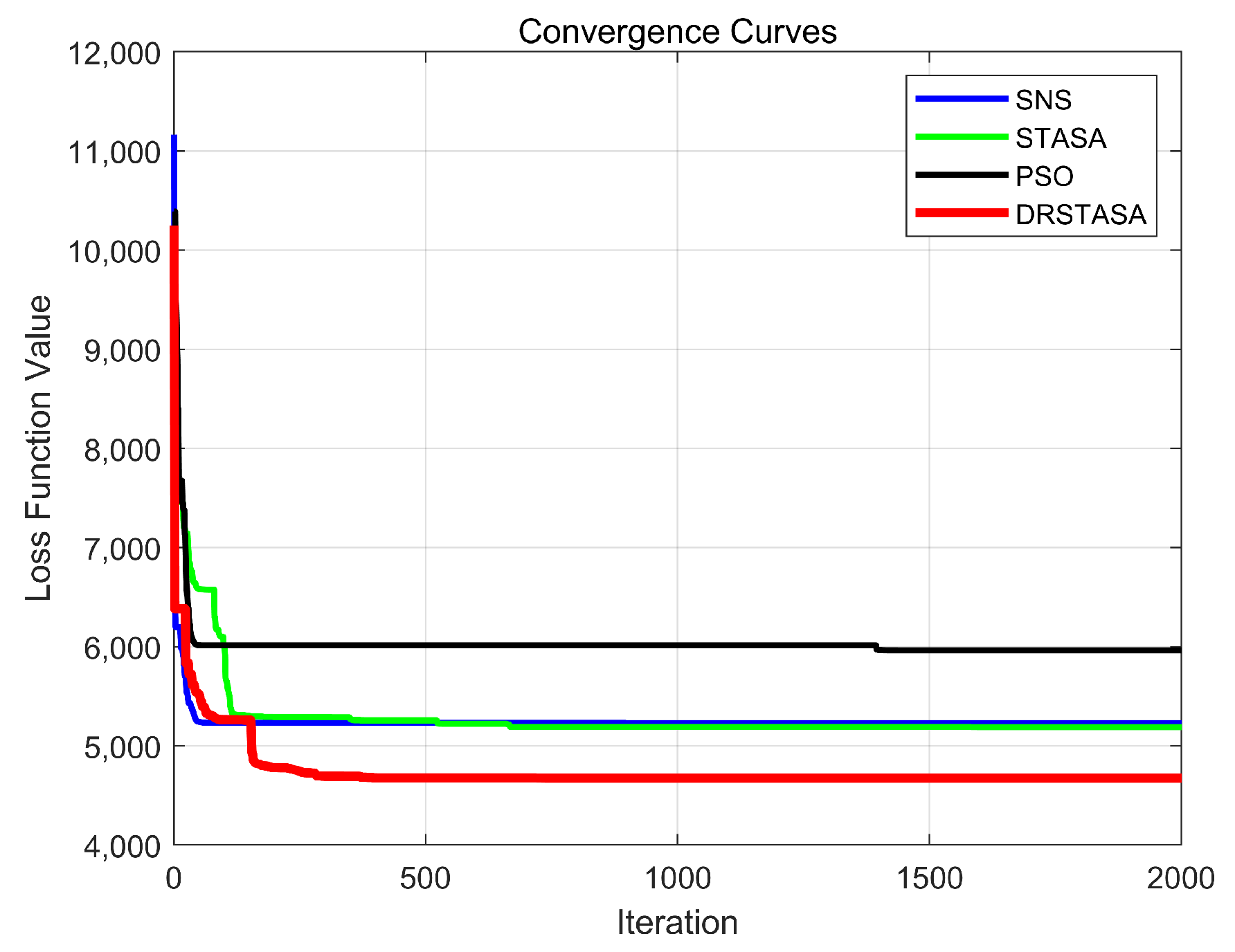
| Algorithm | Optimal Fitness | Worst Fitness | Average Fitness |
|---|---|---|---|
| DRSTASA | 4673.5174 | 5195.8919 | 4737.651 |
| STASA | 4793.8431 | 5485.7753 | 4902.3325 |
| SNS | 4811.4688 | 5934.1597 | 5005.4432 |
| PSO | 4966.2653 | 5857.1326 | 5211.4123 |
Disclaimer/Publisher’s Note: The statements, opinions and data contained in all publications are solely those of the individual author(s) and contributor(s) and not of MDPI and/or the editor(s). MDPI and/or the editor(s) disclaim responsibility for any injury to people or property resulting from any ideas, methods, instructions or products referred to in the content. |
© 2025 by the authors. Licensee MDPI, Basel, Switzerland. This article is an open access article distributed under the terms and conditions of the Creative Commons Attribution (CC BY) license (https://creativecommons.org/licenses/by/4.0/).
Share and Cite
Liu, J.; Han, X.; Liu, F.; Wu, J.; Zhang, W. UAV Path Planning Using a State Transition Simulated Annealing Algorithm Based on Integrated Destruction Operators and Backward Learning Strategies. Appl. Sci. 2025, 15, 6064. https://doi.org/10.3390/app15116064
Liu J, Han X, Liu F, Wu J, Zhang W. UAV Path Planning Using a State Transition Simulated Annealing Algorithm Based on Integrated Destruction Operators and Backward Learning Strategies. Applied Sciences. 2025; 15(11):6064. https://doi.org/10.3390/app15116064
Chicago/Turabian StyleLiu, Jianping, Xiaoxia Han, Fengyi Liu, Jinde Wu, and Wenjie Zhang. 2025. "UAV Path Planning Using a State Transition Simulated Annealing Algorithm Based on Integrated Destruction Operators and Backward Learning Strategies" Applied Sciences 15, no. 11: 6064. https://doi.org/10.3390/app15116064
APA StyleLiu, J., Han, X., Liu, F., Wu, J., & Zhang, W. (2025). UAV Path Planning Using a State Transition Simulated Annealing Algorithm Based on Integrated Destruction Operators and Backward Learning Strategies. Applied Sciences, 15(11), 6064. https://doi.org/10.3390/app15116064