A Robust Methodology for Dynamic Proximity Sensing of Vehicles Overtaking Micromobility Devices in a Noisy Environment

Abstract

The safety of cyclists, e-scooters, and micromobility devices in urban environments remains a critical concern in sustainable urban planning. A primary factor affecting this safety is the lateral passing distance (LPD) or dynamic proximity of motor vehicles overtaking micromobility riders. Minimum passing distance laws, where motorists are required to maintain a minimum distance of 1.5 m when passing a cyclist, are difficult to enforce due to the difficulty in determining the exact distance between a moving vehicle and a cyclist. Existing systems reported in the literature are invariably used for research and require manual intervention to record passing vehicles. Further, due to the dynamic and noisy environment on the road, the collected data also need to be manually post-processed to remove errors and false positives, thus making such systems impractical for use by cyclists. This study aims to address these two concerns by providing an automated and robust framework, integrating a low-cost, small single-board computer with a range sensor and a camera, to measure and analyze vehicle–cyclist passing distance and speed. Preliminary deployments in Singapore have demonstrated the system’s efficacy in capturing high-resolution data under varied traffic conditions. Our setup, using a Raspberry Pi 4, LiDAR distance sensor, a small camera, and an automated data clustering technique, had a high success rate for correctly identifying the number of close vehicle passes for distances between 1 and 1.5 m. The insights garnered from this integrated setup promise not only a deeper understanding of interactions between motor vehicles and micromobility devices, but also a roadmap for data-driven urban safety interventions.

1. Introduction

The shift toward micromobility in urban commuting is a global phenomenon. Driven by environmental concerns, health advantages, and economic factors, urban centers worldwide have seen an uptick in the use of bicycles, e-cargo bikes, and other micromobility devices. The advantages of cycling have been widely recognized and documented, encompassing not only health benefits but also environmental benefits that reduce pollution and traffic congestion [1]. Bicycles, being zero-emission vehicles, offer a tangible solution to mitigate the detrimental environmental impacts traditionally associated with vehicular transportation [2]. Furthermore, in cities like Singapore, where car ownership costs are soaring, cycling offers both an eco-friendly and financially sound alternative.

With the rise in cycling, there has been an unfortunate increase in cycling-related accidents. The World Health Organization reports that 41,000 cyclists face fatal accidents annually during commutes [3]. In Singapore, the growth of food delivery services necessitates more cyclists on the road, further escalating the risk. Data reflect an 11% increase in food consumed/ordered via food delivery services during the COVID-19 pandemic [4] which corresponds to a 25% rise in cycling-related accidents during the same period [5]. Nonetheless, many European countries and the USA, Canada, and Australia, where cycling is prevalent, have resisted effective techniques like traffic calming to improve the safety of cyclists and road safety in general [6]. In fact, there seems to be very little that cyclists can do to prevent vehicles from overtaking them dangerously [7], which suggests that structural or legal measures must be taken to reduce cycling-related accidents.

To address the safety concerns, some cities, including Singapore, have set a 1.5 m passing distance guideline [8]. However, the effectiveness and enforcement of these guidelines remain contentious. Moreover, a study from Germany showed variable adherence levels, where cars meet the legal passing distance of 1.5 m only 30% of the time [9]. Table 1 shows different countries and their different mandatory passing distance (MPD) rules.

Table 1. Countries with a minimum passing distance guideline or law.

Country	MPD Advised	MPD Mandated
Austria	Yes—1.5 m	No
Belgium	No	Yes—1 m
Chile	Yes—1.5 m	No
France	No	Yes—1 m on roads with ≤50 km/h speed limit, and 1.5 m on roads with >50 km/h speed limit.
Germany	No	Yes—1.5 m in urban areas, and 2 m out of town.
New Zealand	Yes—1.5 m	No
Singapore	Yes—1.5 m	No
United States	Yes—varies by state	Yes—varies by state

Note. Table containing the mandatory passing distance rules for various countries [10]).

Despite guidelines, adherence remains an issue. Uncertainty about distance measurements from motorists and a lack of quantifiable evidence from cyclists create complications. Measuring the lateral passing distance of vehicles passing cyclists involves several technical challenges, primarily because it requires accurate, real-time data collection in a dynamic, outdoor environment. The quality of the measured data is influenced by factors including sensor precision, lighting conditions, and the vibration of the moving bicycle.

Current studies, while emphasizing the impact and nature of LPD in their research, do not place enough emphasis on their methods of collection. Data collection of existing studies, which is difficult to replicate, often relies on manual, labor-intensive, and costly equipment. Table 2 depicts a sample of LPD studies conducted in the last decade, the majority of which employ manual collection techniques, relying on an operator to filter through video footage and identify the passing distances of vehicles. Some studies by Lee et al. and Balanovic et al. [11,12] overcame this challenge by relying on a push button that participants could press to identify a vehicle pass. However, this detracts from the authenticity of the riding experience and may also be prone to inaccuracies on the part of the participant. Of the studies that employ automated data collection, many use expensive and complicated setups like a driving simulator such as Herrera et al. [13] and Bella and Silverstri [14], or a difficult-to-replicate setup consisting of expensive and inaccessible equipment like Chuang et al. [15]. Current devices such as the C3FT [16] are available commercially for use in enforcement, education, and research, such as by Feizi et al. [17]. However, the C3FT costs USD $1480 as of 2024 and had to be supplemented with video footage in the study in which it was used. Other studies that use automated collection techniques face difficulties with filtering noise like Schepers et al. [18], or do not describe in-depth the challenges of filtering out false positives, and eliminating spurious data such as Mackenzie et al. [19]. The studies listed above undoubtedly provide comprehensive data analysis and conclusions as to LPD. But while their focus mainly concerns the implications of the data collected, this study aims to investigate the potential of an automated data collection method that reduces manual effort, offering a solution for policymakers, researchers, and consumers. Through the integration of a distance sensor, microcontroller, and an AI camera with computer vision capabilities, we ensure automatic and precise data recording. Post-collection, a clustering analysis technique identifies vehicle passes while filtering out false positives, thereby providing a clear count of close encounters. Additionally, image recognition capabilities of the AI camera in conjunction with the distance sensor enables the accurate determination of vehicles’ relative passing speeds.

Table 2. A comparison of setups used by different research papers.

Reference	Setup	Data Collection Technique
Parkin and Meyers [20]	Video footage with “screen ruler”.	Manual
Mehta et al. [21]	Ultrasonic sensors, GPS receiver, and video camera.	Manual
Balanovic et al. [12]	LiDAR sensors, video camera, GPS, and event button.	Manual
Love et al. [22]	Video footage.	Manual
Walker et al. [7]	Ultrasonic sensor (10 Hz), Arduino, event button.	Manual
Chuang et al. [15]	Global positioning system, ultrasonic sensors, 5 car video camera DVR black boxes, 8 proximity switches, variable resistor, multi-function logger.	Semi-automatic
Bella and Silverstri [14]	Driving simulator.	Automatic
Dozza et al. [23]	2 video cameras, GPS, LiDAR sensor (20 Hz).	Manual
Llorca et al. [24]	3 Video cameras, GPS tracker, laser sensor, laptop, laser pointer.	Manual
Beck et al. [25]	Video camera, ultrasonic sensor (10 Hz).	Manual
Mackenzie et al. [26]	Microcontroller, GPS, 2 ultrasonic sensors (20 Hz), motion sensor.	Automatic
Herrera et al. [13]	Driving simulator.	Automatic
Lee et al. [11]	LiDAR sensor, push button.	Manual
Nolan, et al. [27]	Ultrasonic sensors (25 Hz), Arduino, and two Garmin video cameras.	Manual
Feizi, et. al. [17]	GoPro, C3FT.	Semi-automatic
Mackenzie et al. [19]	2 ultrasonic sensors (20 Hz), microcontroller, GPS.	Automatic
Ivanišević et al. [28]	Ultrasonic sensor, video camera.	Manual
Schepers et al. [18]	LiDAR sensor, GPS, Arduino microcontroller.	Automatic

Our system is mounted on a bicycle and identifies vehicles passing within 1.5 m or closer without requiring manual logging or video cross-referencing. Our results show that through judicious application of signal processing techniques to noisy data and images captured by relatively low-cost hardware, we can achieve a robust system for accurately measuring lateral passing distances and speeds [29,30], with the total cost of our setup being around USD 200. Preliminary testing of our system has shown that it successfully and accurately filters out noise and spurious data to identify close vehicle passes at the range of 1–1.5 m.

2. Methodology

We start by reviewing various distance measuring sensors: laser, LiDAR, and ultrasound. These were assessed for accuracy, range, and reliability through tests against a stationary wall at varying distances. From this evaluation, we selected the most suitable candidates for outdoor experiments. In our outdoor test, the sensors were attached to a stationary bike on the roadside to gauge their proficiency at detecting passing vehicles. Our preferred choice was then integrated with the OAK-1 AI camera and mounted on a bicycle. Real-world data collection was simulated as the bike navigated actual roads with traffic. The system was programmed with Python using the Raspberry Pi, employing modules like Pyserial and Smbus to facilitate communication between the sensors and the Pi. The AI camera was programmed through the DepthAI API by Luxonis. Post-data collection, noise was filtered out to emphasize clusters indicative of vehicle passes. Finally, the machine learning clustering method DBSCAN was employed to automatically identify vehicle passes in the data collected, the accuracy of which was validated using GoPro footage.

3. Sensor Selection

To ensure a robust and accurate data collection system, our study employed an iterative process of selection, testing, and deployment of three types of measuring sensors. The methodology consisted of preliminary indoor and outdoor tests, followed by on-road stationary and mobile tests. Table 3 shows a general comparison between the different types of sensors available. From this comparison alone, it is difficult to determine which type or model of sensor is the most appropriate. Hence, the tests aim to guide our selection.

Table 3. General comparison between different types of sensors.

	LiDAR	Laser	Ultrasonic
Working principle	Uses laser beams to measure distances	Uses a laser beam to measure distance based on reflection	Uses sound waves to measure distances based on echo timing
Range	Typically 100–300 m, but can go up to 1 km for some models	Shorter, often less than 100 m	Typically 2–5 m, though specialized models can go further
Accuracy	±2 cm to ±10 cm depending on model and conditions	±1 mm to ±5 mm	±1 cm for close range but can vary based on conditions
Resolution	Fine; can be sub-cm in some models	Fine, often sub-mm	Coarser, often in the cm range
Pros	High resolution, long-range, works in various lighting conditions	High precision, works in many lighting conditions	Simple, cheap, works in the dark and through many materials
Cons	Expensive, can be affected by atmospheric conditions and reflective surfaces	Range limited, can be affected by reflective surfaces or ambient light	Affected by sound-absorbent materials, less accurate at longer distances

3.1. Indoor and Outdoor Fixed Distance Tests

To determine the compatibility of the sensors with our project’s specific needs, we executed a comprehensive set of tests. Our benchmarks necessitated the precise measurement of distances up to 3 m in outdoor daylight and the capability to detect high-speed vehicular movements.

Table 4 delineates a comparative analysis of various sensors tested, all of which exhibit notable accuracy in detecting vehicles within a maximum distance of 3 m. Despite their evident precision and sufficiently high frequency to execute the task, it is crucial to note that the performance of laser and LiDAR sensors may be compromised under daylight conditions.

Table 4. Comparative specifications of select distance sensors tested.

	WaveShare TOF (WaveShare, Shenzhen, China)	JRT BB2X Laser (Chengdu JRT Meter Technol-ogy Co., Ltd., Chengdu, China)	LiDAR Lite V4 (Garmin, Olathe, KS, USA)	A02YYUW (DFRobot, Shanghai, China)
Sensor type	Laser	Laser	LiDAR	Ultrasonic
Max. range	5 m	100 m	10 m	4.5 m
Frequency	10 Hz	10–20 Hz	200 Hz	10 Hz
Accuracy	±1 cm short/medium distance ±1.5 cm long distance	±3 mm	±1 cm to 2 m ±2 cm to 4 m ±5 cm to 10 m	±1 cm
Affected by light	Yes	Yes	Yes	No

We tested each sensor at fixed intervals of 0.5 m, spanning a range from 0 to 5 m. These tests took place in both internal and external environments to assess sensor performance under varying conditions. At every interval, around 500 distance data points were gathered. The sensors were either operated using their default software or integrated with a Raspberry Pi for control.

The graphs and tables presented in the findings utilize various visual elements to depict sensor performance. Solid dots on each graph represent the average distance recorded by the sensor at specified intervals, while red bars indicate standard deviations.

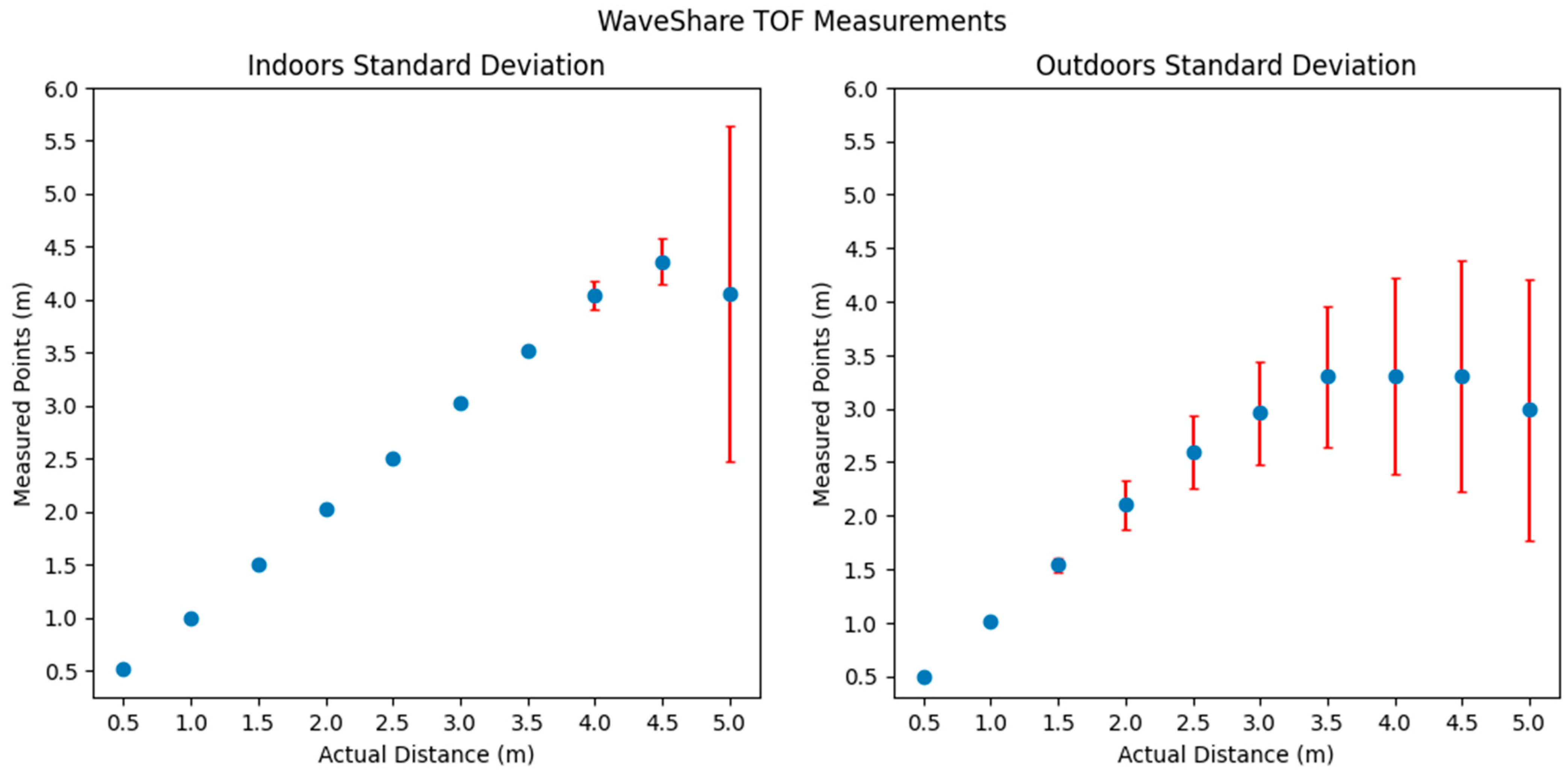
Focusing initially on the WaveShare TOF sensor (Figure 1 and Table 5), it demonstrated reliable performance up to 4.5 m in indoor settings. However, a noticeable decline in accuracy and consistency was observed outdoors, where the standard deviation surged from 0.34 m at a distance of 2.5 m to 1.22 m at 5.0 m.

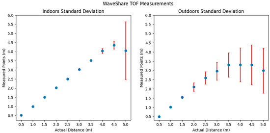
Figure 1. Depicts the mean distance measured by the WaveShare TOF sensor across distances of 0.5 m to 5.0 m. The red bars represent the standard deviation of the measurements at each interval (Yap).

Table 5. Standard deviation of measurements at different intervals for TOF laser range sensor.

	0.5 m	1.0 m	1.5 m	2.0 m	2.5 m	3.0 m	3.5 m	4.0 m	4.5 m	5.0 m
Indoors	0.01	0.01	0.01	0.01	0.01	0.02	0.03	0.14	0.22	1.58
Outdoors	0.00	0.01	0.07	0.23	0.34	0.48	0.66	0.92	1.08	1.22

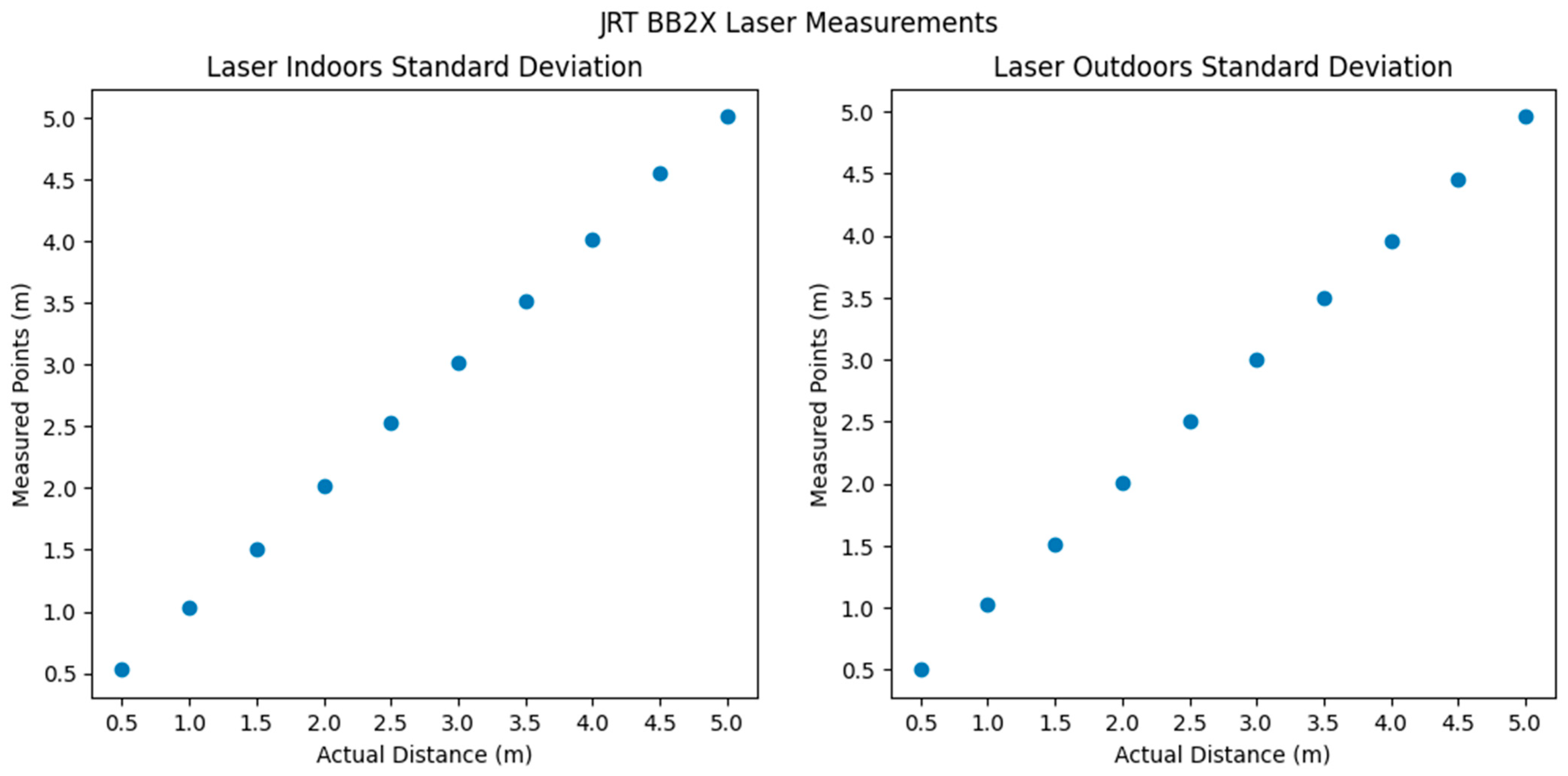
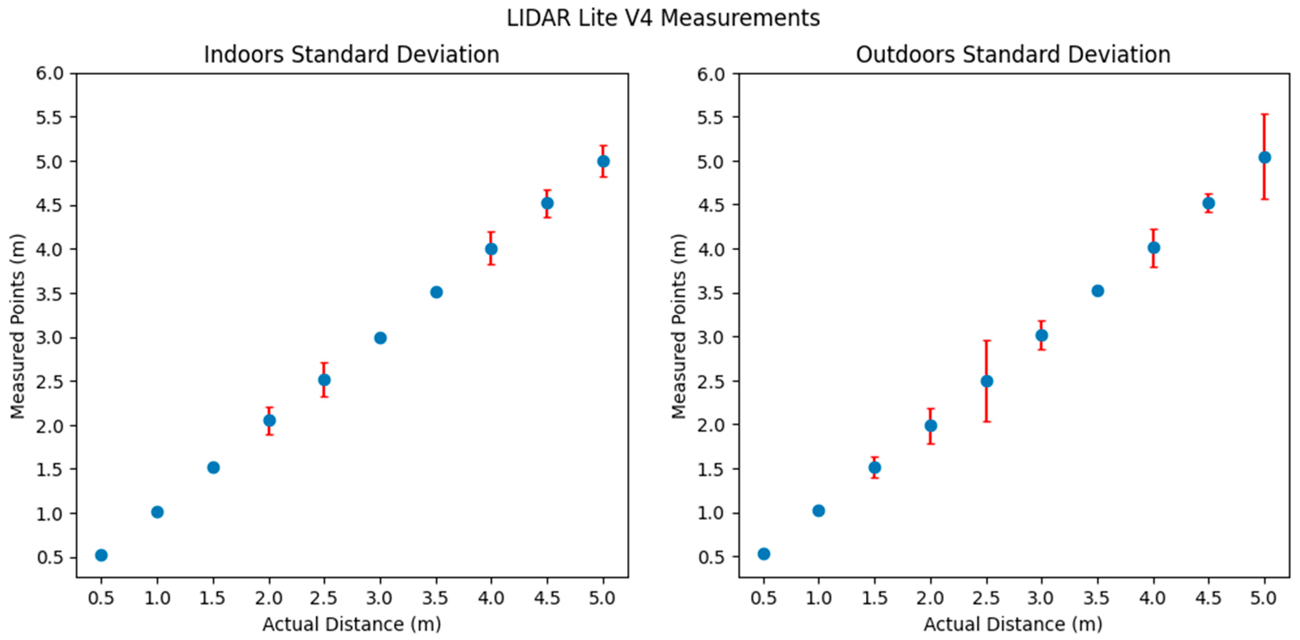
In contrast, both the JRT BB2X Laser and LiDAR Lite V4 sensors maintained accuracy across all tested environments. Notably, the JRT BB2X Laser showcased high precision, with an almost negligible standard deviation, as depicted in Figure 2 and Table 6. Although the LiDAR Lite V4 sensor (Figure 3 and Table 7) manifested accurate readings, it did not match the laser sensor’s precision, with its highest standard deviation being under 0.5 m—still notably superior to the WaveShare TOF sensor.

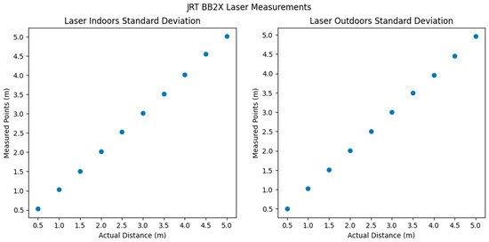
Figure 2. Illustrates the mean distance measured by the JRT BB2X Laser across distances of 0.5 m to 5.0 m. The lack of red bars indicate an extremely small standard deviation.

Table 6. Standard deviation of measurements at different intervals for BB2X JRT Laser.

	0.5 m	1.0 m	1.5 m	2.0 m	2.5 m	3.0 m	3.5 m	4.0 m	4.5 m	5.0 m
Indoors	0.00	0.00	0.00	0.00	0.00	0.00	0.00	0.00	0.00	0.00
Outdoors	0.00	0.00	0.00	0.00	0.00	0.00	0.00	0.00	0.00	0.00

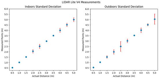
Figure 3. Depicts the mean distance measured by the LiDAR Lite V4 from the 0.5 m to 5.0 m range. The red bars represent the standard deviation of the measurements at each interval.

Table 7. Standard deviation of measurements at different intervals for LiDAR Lite V4.

	0.5 m	1.0 m	1.5 m	2.0 m	2.5 m	3.0 m	3.5 m	4.0 m	4.5 m	5.0 m
Indoors	0.01	0.02	0.05	0.15	0.19	0.03	0.03	0.18	0.16	0.18
Outdoors	0.02	0.02	0.12	0.20	0.46	0.16	0.04	0.21	0.10	0.49

Note. We noticed an anomaly where the standard deviation for the LiDAR Lite V4 sensor around 2.0 m to 2.5 m spikes. This could be due to an internal algorithm in the sensor.

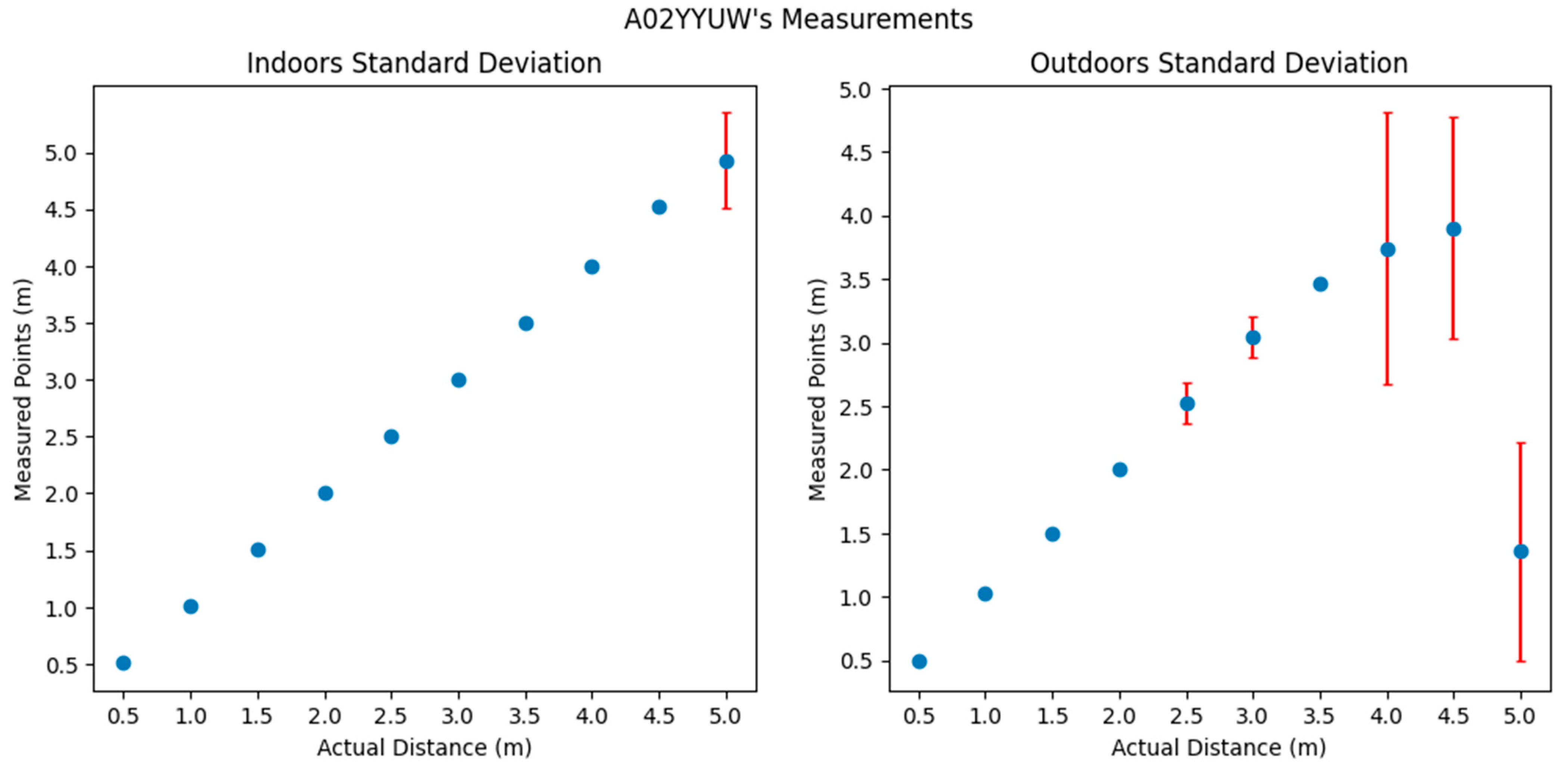
Figure 4 and Table 8 shows that the A02YYUW ultrasonic sensor’s reliability is effective up to 4.5 m and 3.5 m for indoors and outdoors, respectively. Unlike other sensors, its measurement inconsistencies are not due to environmental sunlight conditions but rather its high sensitivity. While dependable at short ranges with a 10 Hz frequency, the sensor’s effectiveness diminishes beyond 2.5 m, demanding precise positioning to accurately capture data. Even slight deviations can lead to entirely incorrect readings. Given these limitations, the A02YYUW’s sensitivity and requirement for exact alignment make it an impractical choice for experiments necessitating robust performance, especially in dynamic settings like motion-based cycling.

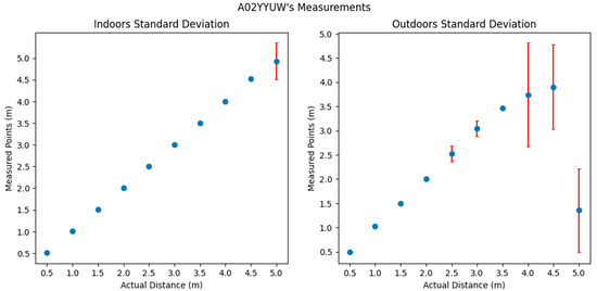
Figure 4. Depicts the mean distance measured by the A02YYUW from the 0.5 m to 5.0 m range. The red bars represent the standard deviation of the measurements at each interval.

Table 8. Standard deviation of measurements at different intervals for A02YYUW.

	0.5 m	1.0 m	1.5 m	2.0 m	2.5 m	3.0 m	3.5 m	4.0 m	4.5 m	5.0 m
Indoors	0.00	0.00	0.00	0.00	0.00	0.00	0.00	0.00	0.00	0.42
Outdoors	0.02	0.02	0.00	0.02	0.16	0.16	0.00	1.07	0.87	0.86

The findings from our tests indicate that the manufacturers’ specifications for the sensors hold true only under optimal conditions. In real-world scenarios, the sensors exhibited increased unreliability, underscoring the necessity of these tests to ascertain whether the sensors meet our criteria.

3.2. Stationary Bike Test

We mounted the sensors onto a stationary bicycle positioned beside a road with moderate traffic. Using a GoPro camera in tandem with each sensor, we assessed their capability to identify passing vehicles. This setup provided insights into the sensors’ performance under controlled yet realistic conditions.

3.2.1. Laser Sensor

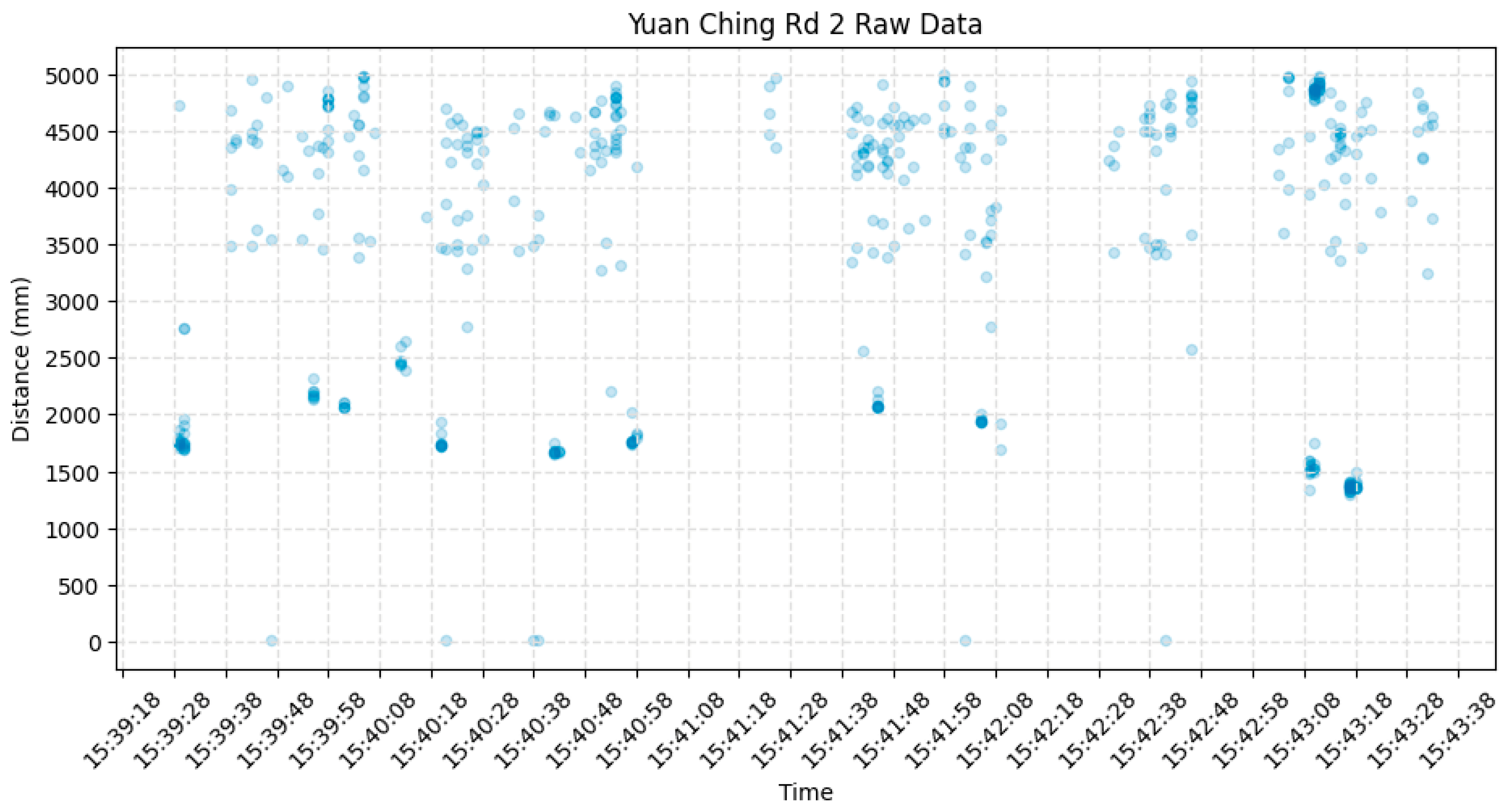
Figure 5 presents the results from the stationary bike test using the JRT BB2X Laser sensor. Despite its high reliability in distance measurement, the sensor’s frequency proved inadequate for accurately recording the distances of passing vehicles, even in moderate traffic. Although the product documentation advertised a frequency of 10–20 Hz, real-world tests showed it to be inconsistent and often much lower.

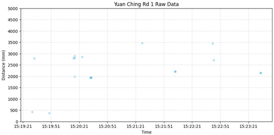
Figure 5. Results from the JRT BB2X Laser sensor’s stationary test.

3.2.2. LiDAR Sensor

The LiDAR sensor, with its impressive frequency reaching up to 200 Hz, was adept at detecting passing vehicles, as evidenced by the clusters of dark points in Figure 6. Having validated the LiDAR sensor’s proficiency, we progressed to the mobile bike assessment.

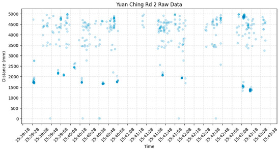
Figure 6. Results from the LiDAR Lite V4′s stationary test.

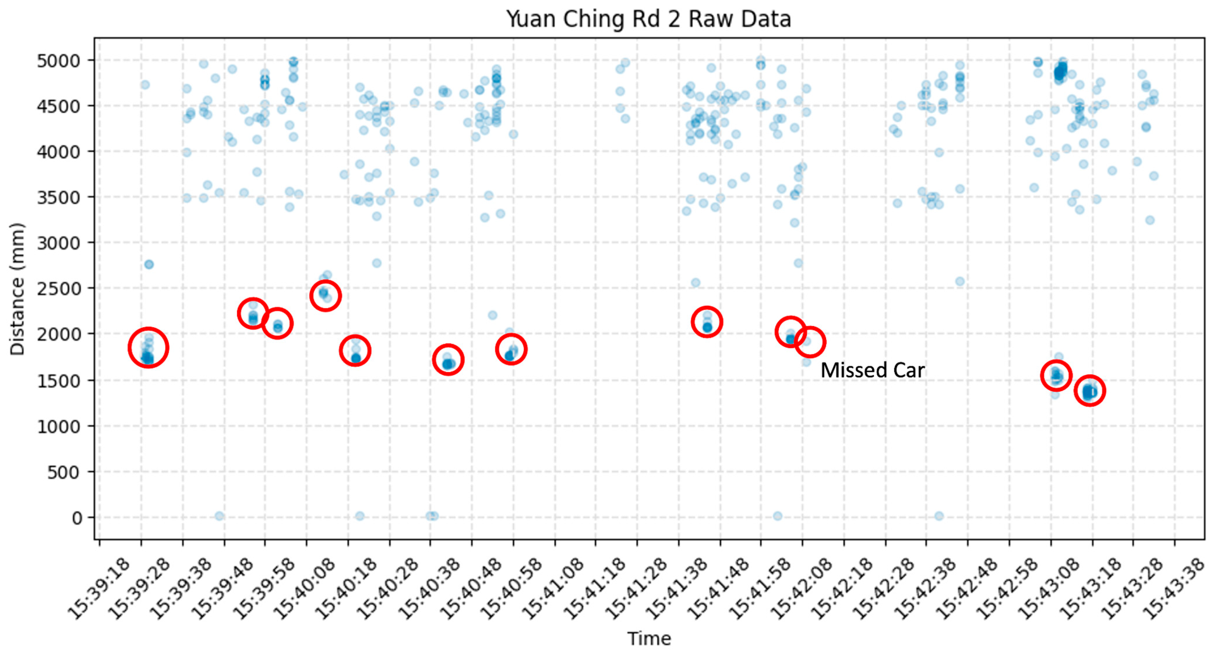
Next, we cross-referenced the video footage from the GoPro with the data collected. Each red circle in Figure 7 highlights the points representing a vehicle pass. Out of 12 vehicles, the sensor only failed to detect a single car at 15:42:08, resulting in an approximate success rate of 92% based on this limited dataset. This confirms that the dark point clusters generated by the sensor indeed represent the passing of vehicles. With this verification, we advance to the final evaluation of the complete setup.

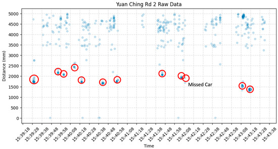
Figure 7. Results from the LiDAR Lite V4′s stationary test annotated. Red circles indicate overtaking vehicles.

4. Mobile Bike Test

To mimic the real-world scenario of a cyclist on the move, our sensor was mounted on a bicycle and cycled along a 5 km route alongside moderate traffic in Singapore’s Jurong West area as shown in Figure 8. This phase aimed to assess the challenges and practicality of each sensor during typical cycling activities.

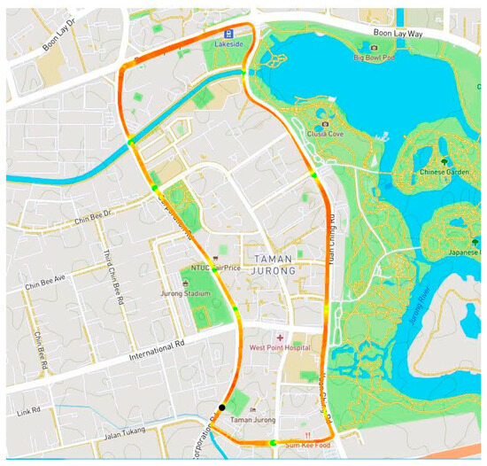
Figure 8. The route cycled for the data collection.

4.1. Setup

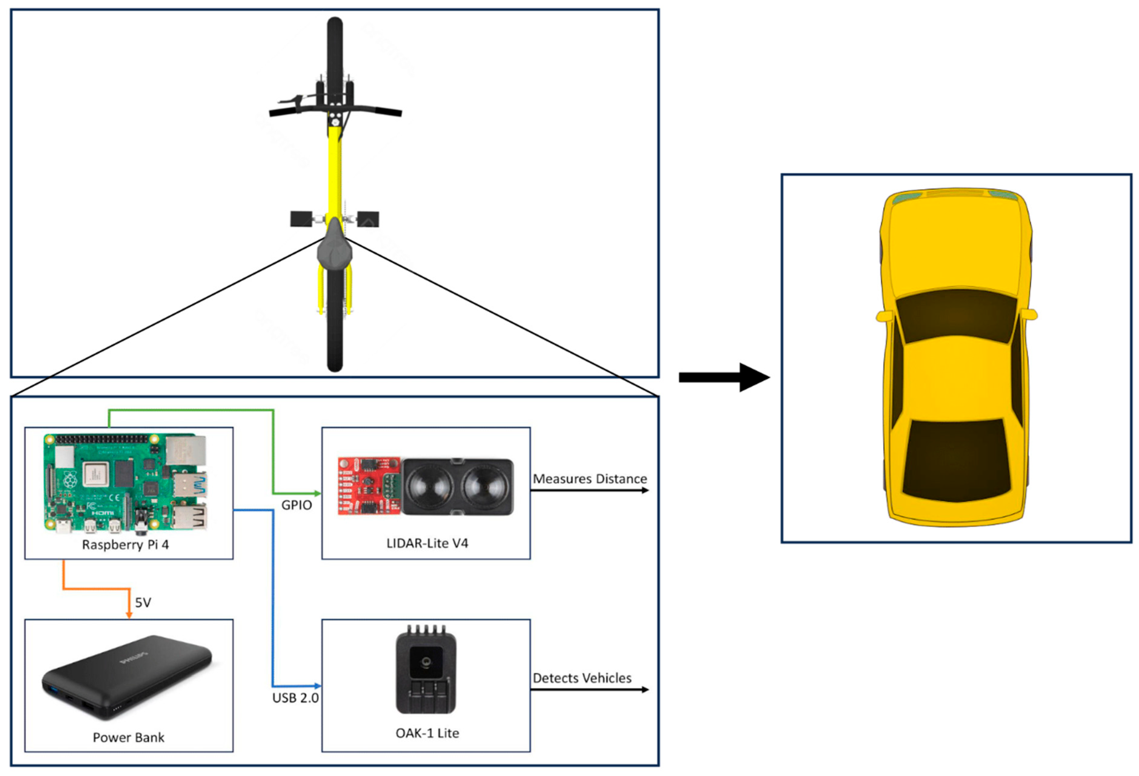
Our configuration integrated three primary components: the LiDAR sensor, a Raspberry Pi with its power supply, and the OAK-1 Lite camera by Luxonis. The schematic in Figure 9 breaks down the components of the setup, which together work to detect passing vehicles, and Figure 10 depicts the final setup mounted on a bike. The principle behind this setup was to leverage the object detection capability of the OAK camera to identify an approaching car in proximity to the cyclist. Upon detection, the LiDAR sensor would activate to record distances. This approach not only streamlined the data collection process but also significantly reduced the occurrence of false positives and irrelevant data. By focusing measurements exclusively during confirmed vehicle presence, we can enhance data accuracy. Unlike other systems, our refined data processing eliminates the need for tedious manual cross-referencing with video footage or reliance on manual interventions like button presses to ascertain data quality. In our initial tests, we also attached a GoPro to the bike to manually cross-check and validate the collected data, as shown in Figure 10. However, the GoPro was not part of the final configuration.

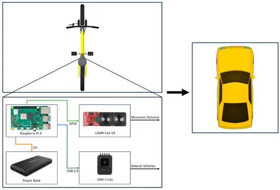
Figure 9. Schematic of the setup.

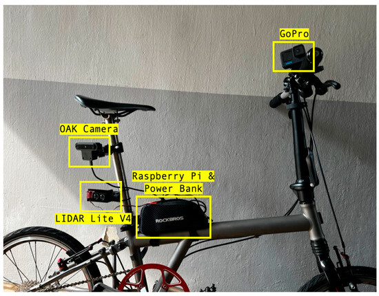
Figure 10. Raspberry Pi, LiDAR Lite V4, and OAK camera mounted on the bike with a GoPro.

4.2. Preliminary Results

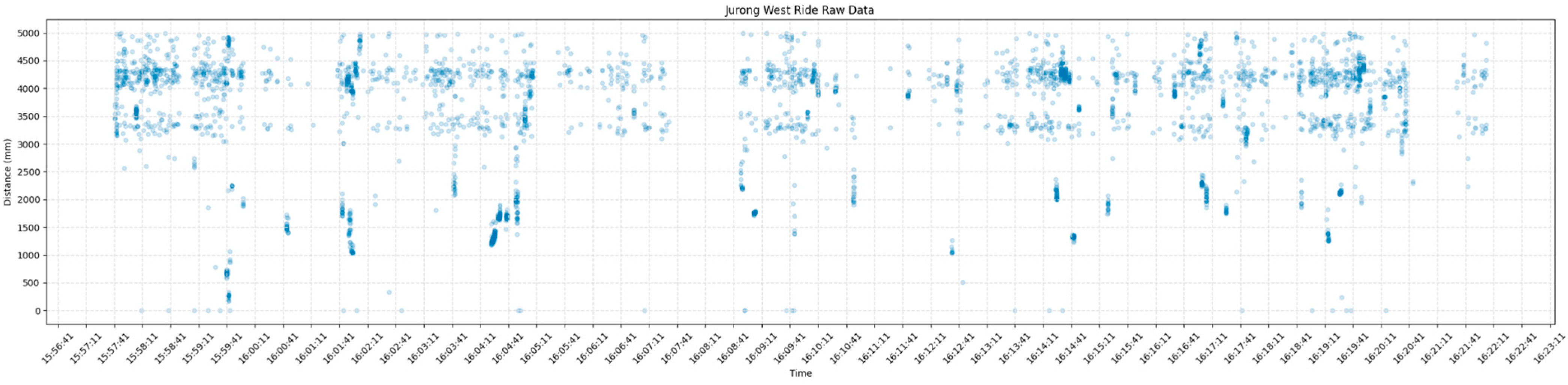
At first glance at Figure 11, the data appeared extremely noisy. However, a detailed look reveals that most of the noise originates from readings above 3 m, which is not important to the experiment, as we are mainly concerned with close vehicle passes. Below this threshold, the data are notably cleaner, with pronounced dark clusters signaling vehicle passes. Interestingly, the broad gaps seen around 16:07:41 signify periods when the AI camera detected no vehicles, which contributed to reducing the overall noise in the dataset.

Figure 11. Raw data collected by the LiDAR Lite V4 in conjunction with the OAK camera.

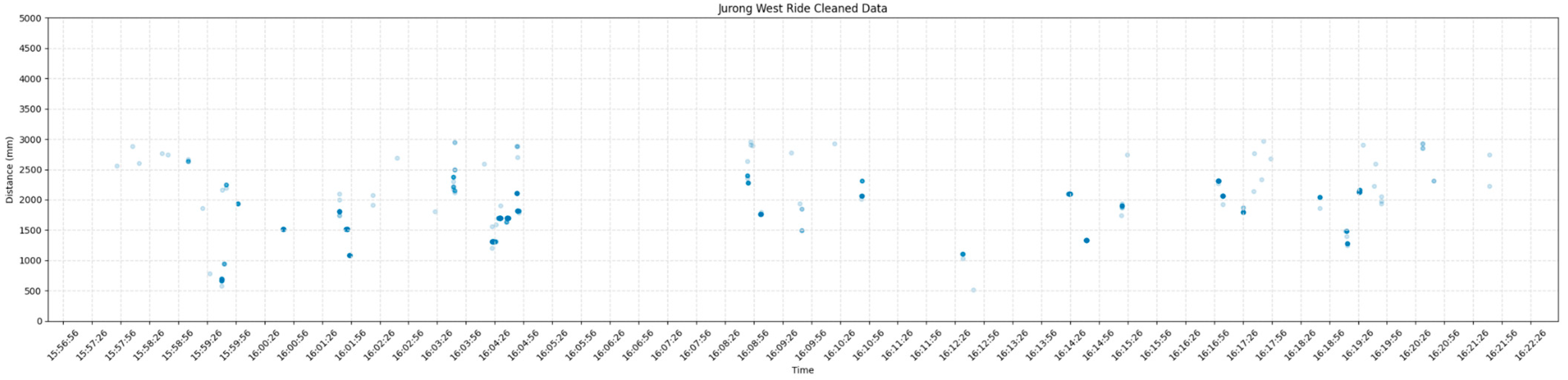
To further clarify our findings, we cleaned our data in Figure 12 by first removing all data points above the 3 m mark. We then accentuated clusters, which are simply a continuous set of non-null data points. We calculated the average of these points and replaced the entire cluster with this average.

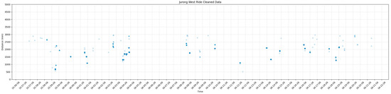
Figure 12. Cleaned data from the LiDAR Lite V4 and OAK camera.

To verify that these dark clusters truly represented vehicles, we cross-referenced our findings with GoPro footage, circling all vehicle passings in red in Figure 13. Overall, the sensor adeptly identified vehicles passing the cyclist. Of the 21 vehicles that overtook the cyclist in the same lane, our setup correctly identified 7 passed at a proximity of 1.5 m or closer. Points not highlighted in red either indicate false positives or noise. The subsequent clustering algorithm will identify false positives, while isolated faint points represent noise.

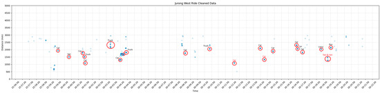
Figure 13. Data collected with LiDAR and OAK camera annotated using GoPro footage. Red circles indicate passing vehicles and are annotated with the type of passing vehicle. Blue circles indicate stopped vehicles that the cyclist overtook.

4.3. Automated Data Analysis

To enhance efficiency in the data collection process, we replaced the time-consuming manual identification of clusters through cross-referencing with the GoPro with an algorithmic approach that automatically recognizes clusters representing vehicle passes.

4.3.1. Clustering Algorithm Selection

The sensor emits measurement signals at a frequency of approximately 20 Hz. Instead of producing one or two random data points, it should record a cluster of points that represent the distance of the overtaking vehicle during its pass. Hence, we require a cluster analysis to automatically identify vehicle passes.

The exploration of clustering algorithms reveals distinct methodologies and applications across various domains, each with unique working principles, cluster determination methods, and optimal use cases [31]. For instance, K-Means, renowned for its application to large datasets with approximately spherical cluster shapes, necessitates a specified number of clusters and exhibits high sensitivity to outliers [32]. Contrastingly, DBSCAN, a density-based algorithm, autonomously determines the number of clusters, showcasing adeptness in identifying clusters of varied shapes and sizes while proficiently managing noise and outliers [33]. Hierarchical clustering, particularly agglomerative clustering, and the Gaussian mixture model (GMM) require a specified number of clusters and demonstrate moderate sensitivity to outliers, with the former being suitable for small datasets requiring a tree-like structure and the latter being apt for scenarios demanding probabilistic cluster assignments [34,35]. Mean shift, a mode-seeking algorithm, determines clusters automatically and is notably utilized in computer vision and image segmentation [36]. Table 9 provides a brief comparison between the different clustering algorithms available.

Table 9. General comparison between different types of clustering algorithms.

	Working Principle	Number of Clusters	Sensitivity to Outliers	Use Cases
K-Means	Partitioning	Needs to be specified	High	Large datasets: when the shape of clusters is approximately spherical.
DBSCAN	Density-based	Determined automatically	Low	When cluster shape is irregular, and noise/outliers are present.
Hierarchical	Agglomerative or divisive	Visualized using dendrogram, cut at desired level	Moderate	Small datasets: when tree-like structure or hierarchy is required.
Agglomerative	Groups data into objects into a tree of clusters.	Needs to be specified	Moderate	When a hierarchical approach is desired.
Gaussian Mixture Model (GMM)	Uses probability distributions	Needs to be specified	Moderate	When clusters are elliptical or when probabilistic cluster assignments are desired.
Mean Shift	Mode seeking	Determined automatically	Moderate	Image segmentation, computer vision.

For the specific task of identifying close vehicle passes, DBSCAN emerges as a preferred choice among clustering algorithms. Unlike K-Means or Gaussian mixture models, DBSCAN does not require a predefined number of clusters, making it adept at discovering clusters of varied shapes and sizes. Moreover, DBSCAN’s inherent ability to segregate noise or outliers ensures that sporadic, unrelated data points do not form erroneous clusters, a challenge that can affect some other algorithms. This noise-handling capability makes DBSCAN particularly suited for real-world data where outliers are common. For a dynamic setting like traffic with unpredictable passing patterns and potential anomalies, DBSCAN offers the robustness and adaptability necessary to discern meaningful clusters effectively.

4.3.2. DBSCAN

Given a set of points in some space, DBSCAN groups together points that are closely packed together (points with many nearby neighbors), marking as outliers points that lie alone in low-density regions.

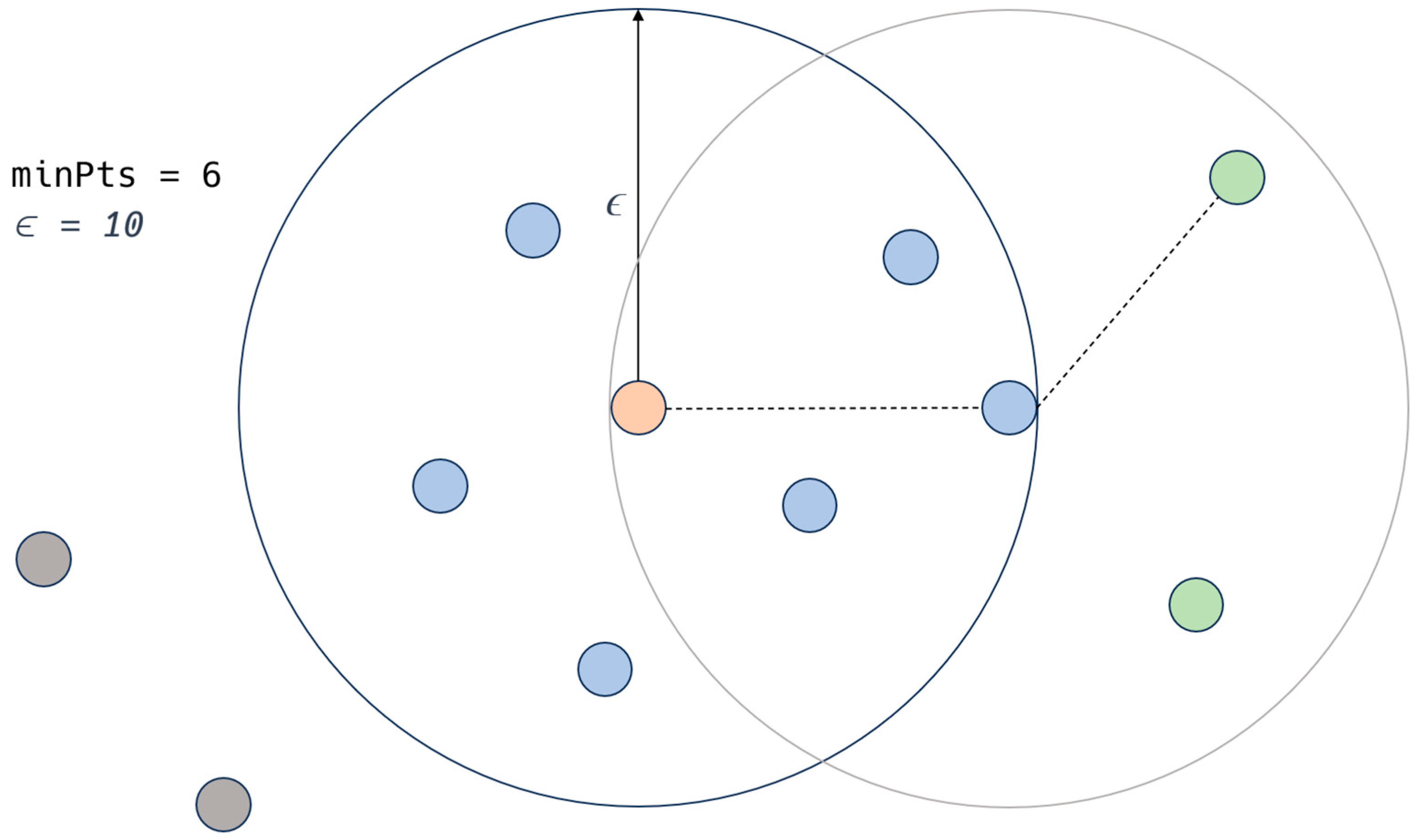
Let $D$ be the dataset of all points, $Q$ be the query point, and $N\left(Q\right)$ represent the neighborhood of $Q$, which includes all points within distance ε of $Q$.As illustrated in Figure 14 by the orange point, a point $Q$ is a core point if at least $minPts$ points are within distance ε of it.

$$Q \mathrm{is} \mathrm{a} \mathrm{core} \mathrm{point} \mathrm{if} \left|N\left(Q\right)\right|\ge minPts$$

(1)

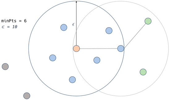
Figure 14. DBSCAN illustration. Peach point represents a core point which forms the main part of a cluster. Blue points are border points which have fewer than minPts within radius ε. Gray points refer to noise. Green points are border points belonging to different clusters.

A point $P$ is directly reachable from $Q$ if point $P$ is within distance ε from core point $Q$, shown by the blue points to the orange point.

$$P \mathrm{is\; directly\; reachable\; from} Q \mathrm{if} P\in N\left(Q\right) \mathrm{and} \mid N\left(Q\right)\mid \ge minPts$$

(2)

As illustrated by the green points, point $P$ is reachable from $Q$ if there exists a sequence of points:

$$p_1, p_1,\dots ,p_n \mathrm{with} p_1=Q \mathrm{and} p_n=P,\mathrm{where} p_{i+1} \mathrm{is} \mathrm{directly} \mathrm{reachable} \mathrm{from} p_i$$

(3)

Formally, a cluster in DBSCAN is a non-empty subset $C \subseteq D$ satisfying the following:

• For any two points $P$ and $Q$ in $C$, if $Q$ is reachable from $P$, then $P$ and $Q$ are part of the same cluster.
• For any point $Q$ in $C$, if there is a point $P$ in $C$ such that $Q$ is reachable from $P$, and $P$ is a core point.

All other not reachable points are considered outliers or noise as indicated by the gray points and can be represented as follows:

$$D\backslash {\bigcup }_{all clusters C} C$$

(4)

Therefore, the DBSCAN algorithm can be understood as a region query, where $Nϵ\left(p\right)$ is the ε-neighborhood of the point $Q$ in dataset D:

$$N_{ϵ}\left(Q\right)=\left\{P \in D \mid dist\left(Q,P\right) \le ϵ\right\}$$

(5)

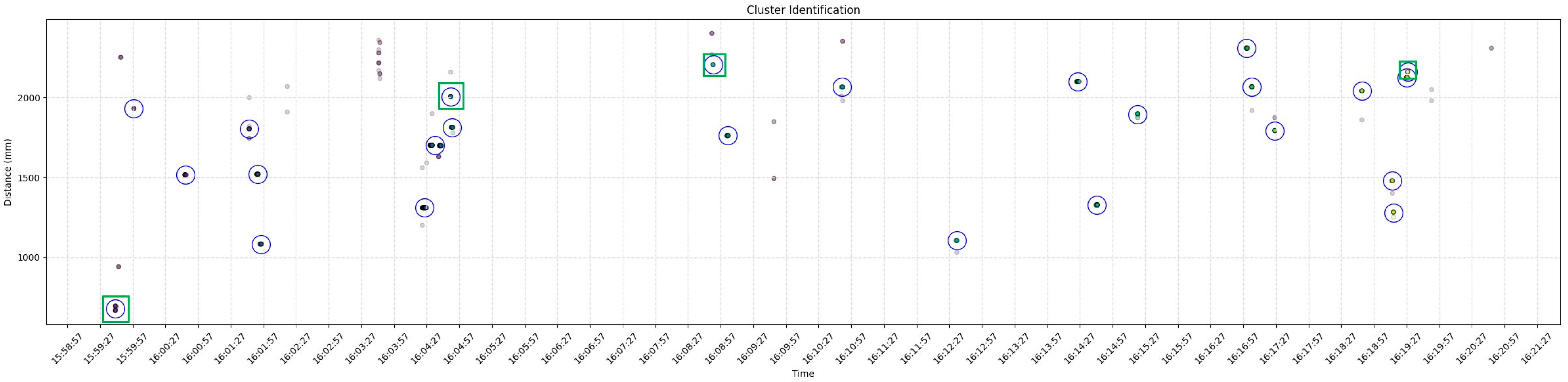
In our experiment, we calibrated ε to 0.02 and $minPts$ to 6. The results, as shown in Figure 15, depict the clusters identified by DBSCAN circled in blue, which represent vehicle passes. There were four false positives detected by the algorithm, as marked with green squares, with the remaining points being noise. However, when distinguishing close vehicle passes ranging from 1 m to 1.5 m, DBSCAN demonstrated 100% accuracy. Clusters indicating passes under 1 m are assumed to be anomalies, given the low likelihood of such close overtakes. Similarly, passes over 2 m likely belong to vehicles in different lanes, and these can also be filtered. Therefore, with our preliminary results, we show that it is possible to create an automated framework that easily collects and analyzes close vehicle passes with no reliance on manual techniques.

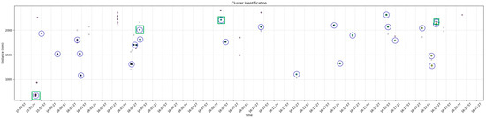
Figure 15. Clusters identified using DBSCAN. Green squares indicate false positives.

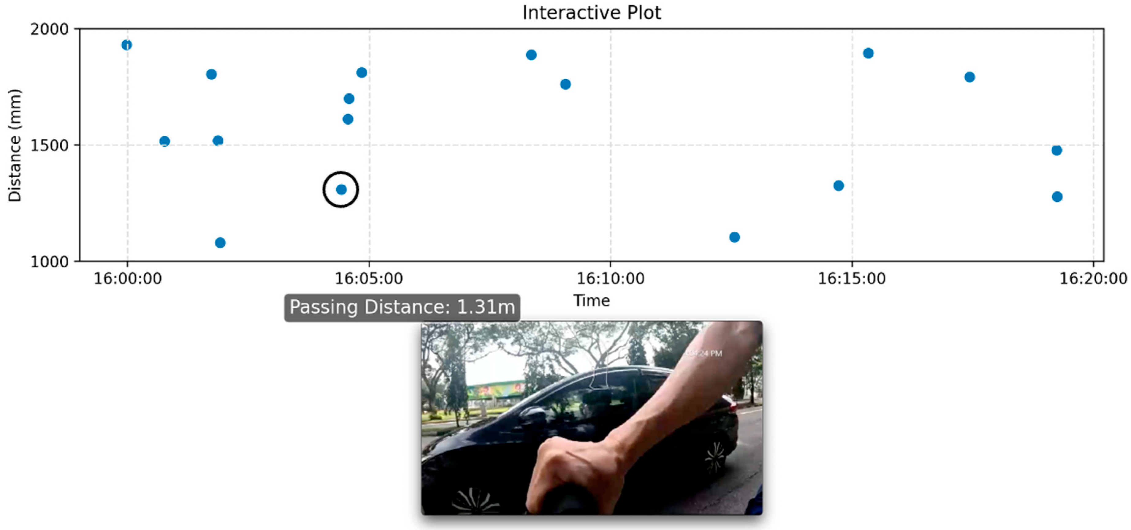
Using DBSCAN, we isolated points between 1 m to 2 m and averaged each cluster to represent a vehicle pass with a single point on a scatter plot. We then extracted relevant screenshots from the GoPro video and integrated them into an interactive plot. Users can click on a point to view the corresponding overtaking vehicle screenshot and its passing distance. In Figure 16, the clicked point is highlighted with a black circle, showcasing an overtaking car at that specific distance.

Figure 16. Interactive plot depicting a vehicle overtaking at 1.31 m.

5. Speed Considerations

Our system further implements the capability to monitor the speed of passing vehicles. Considering that some countries adjust passing distance rules based on vehicle speed, this feature is significant and would offer deeper insights into cyclist and vehicle safety interactions.

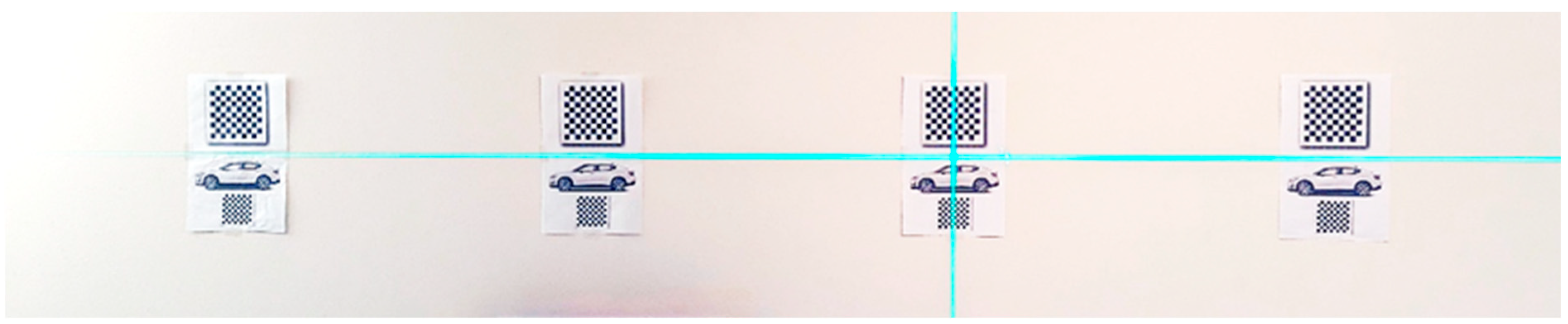
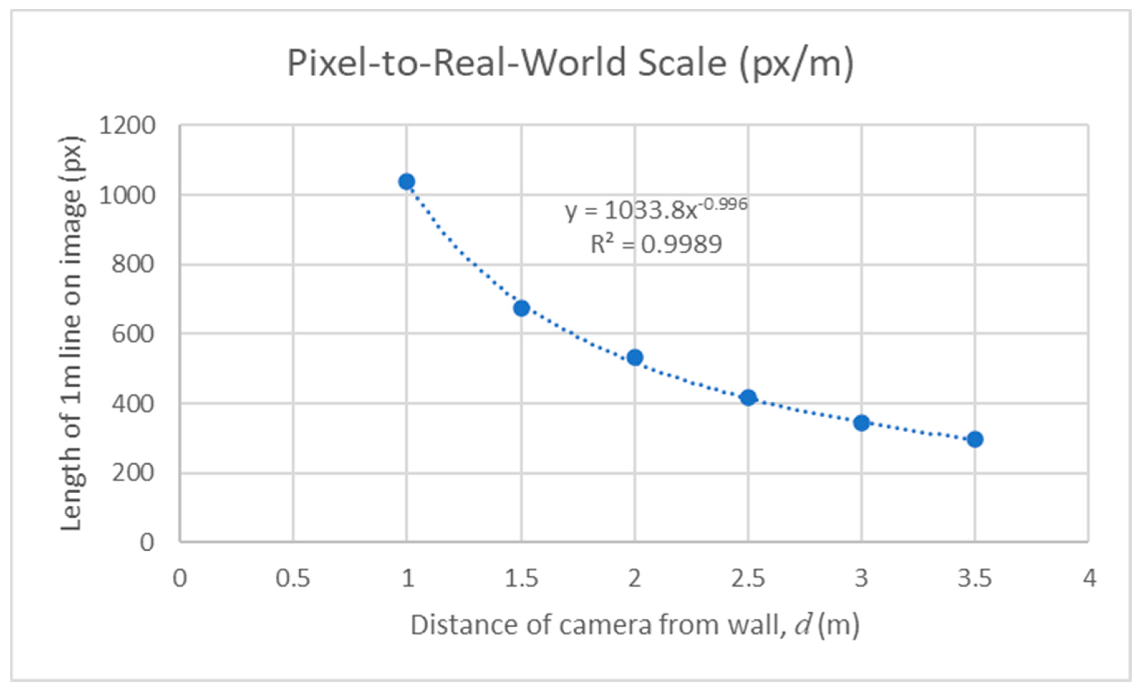
To estimate the speed of a passing car from video footage, we first need to determine the pixel-to-real-world scale for the different passing distances between the bike (on which the camera is mounted) and the car. This can be carried out by measuring a known object in the image and then dividing the pixel length of the object by its real-world length. The pixel-to-real-world scale is inversely proportional to the distance of the camera from the object. From an experiment using an OAK-1 camera and equally spaced checkerboard images on a vertical wall as shown in Figure 17, we show that the number of pixels on a camera image that corresponds to a horizontal line of length 1 m is almost inversely proportional to the distance of the camera from the wall, $d$ in Figure 18.

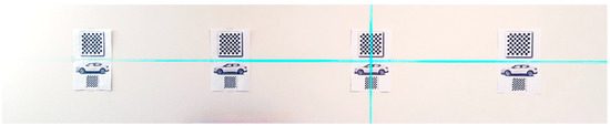
Figure 17. Checkerboard images at 1 m horizontal spacing on a vertical wall. The cyan laser lines are used to guide the placement of images.

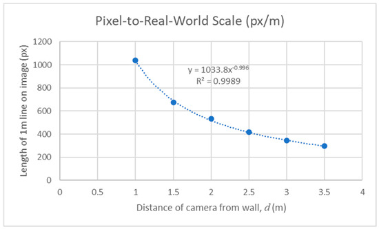
Figure 18. A trend line through the data points shows a near-perfect inverse relationship between pixel-to-real-world scale and working distance.

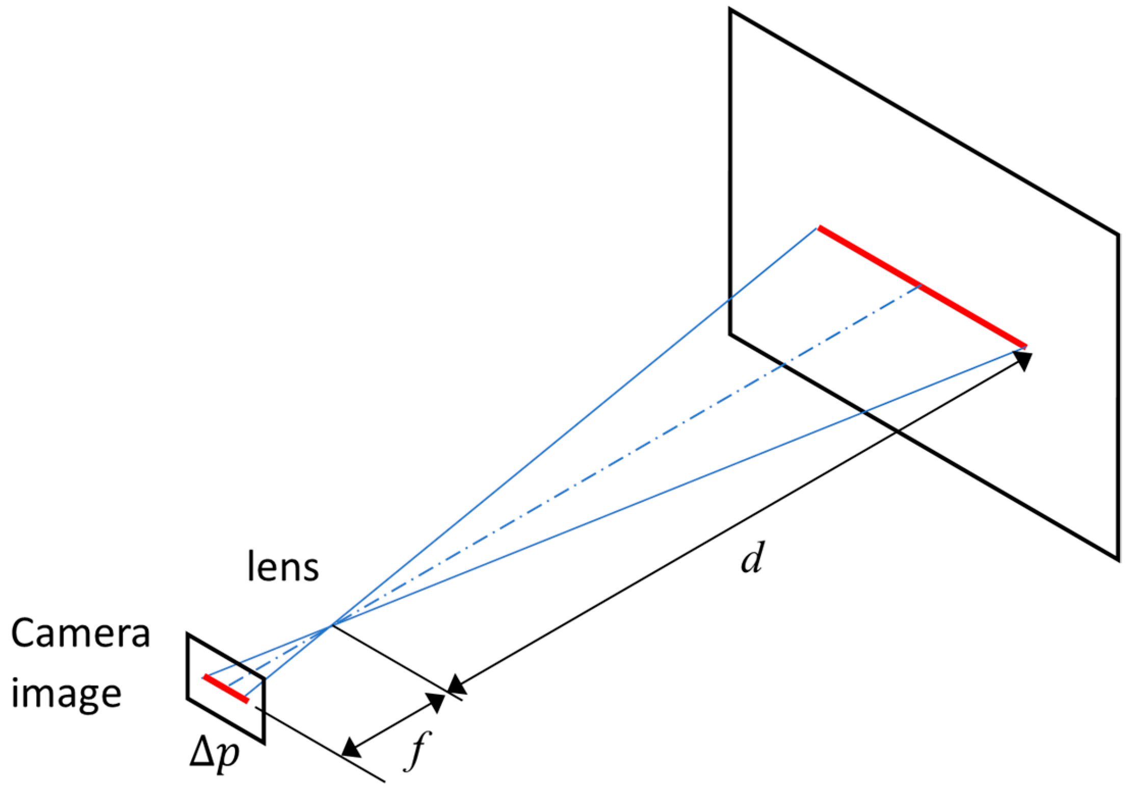
Thus, for any horizontal displacement of length $\mathsf{\Delta }p$ pixels on an OAK-1 camera image, the actual displacement, $s$, as illustrated in Figure 19, is given as follows:

$$s=\mathsf{\Delta }p\left(\frac{1}{f}d\right)=\mathsf{\Delta }p\left(\frac{1}{1033.8}d\right)$$

(6)

where $d$ is the distance between the camera and the car, and f is the focal length of the camera, which can be determined from a regression analysis of the experimental data.

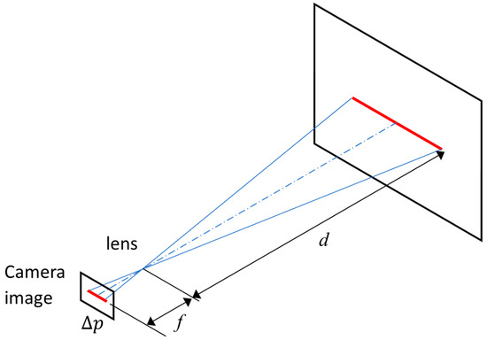
Figure 19. Camera projection model.

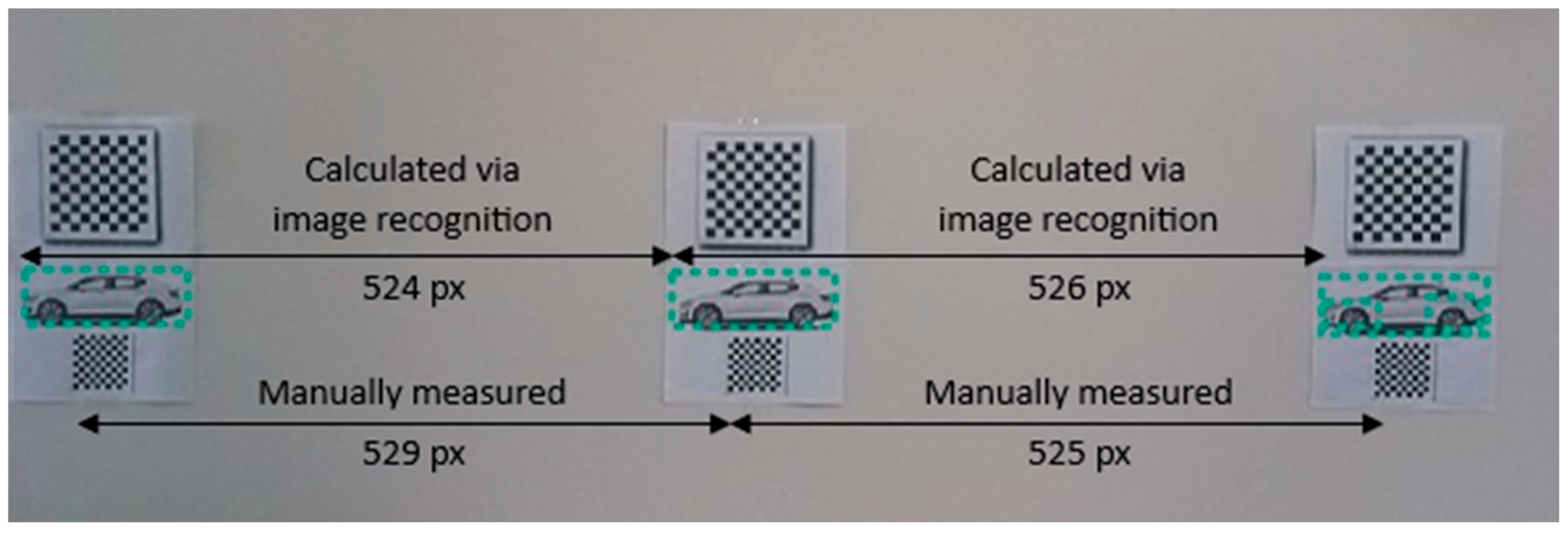
From video footage of a passing car, we can extract the image frames and the time of each frame. We can then calculate the displacement of the car, $s$, between any two frames using Equation (6). The speed of the car relative to the bike, v, can be estimated by using $v=\frac{s}{\mathsf{\Delta }t}$, where $\mathsf{\Delta }t$ is the time difference between the two frames. The speed estimation can also be performed automatically using image recognition by tracking the displacement of the bounding box of the passing car (or part of the car such as the front wheel). Figure 20 highlights the minor discrepancies between manually measured distances in car images and those computed through image recognition. From experiments, the errors in the displacement estimates are less than 5%. This works out to be 2 km/h for a relative speed of 40 km/h.

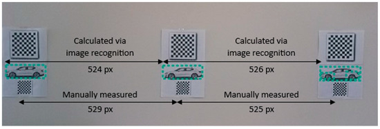
Figure 20. Comparing manually measured and image recognition-calculated displacements.

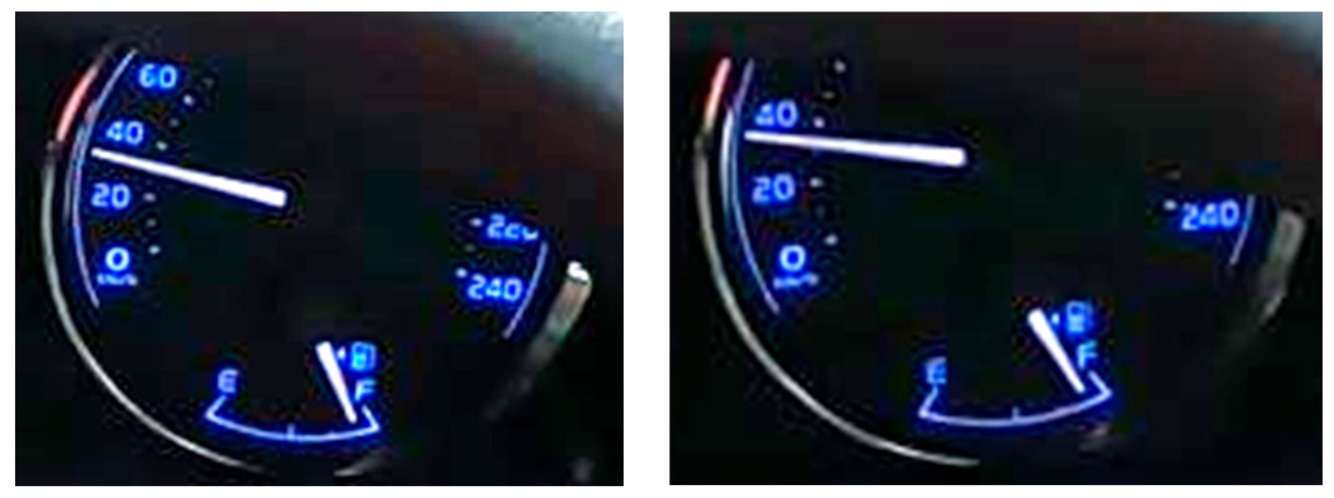
Figure 21 shows an experiment to estimate the speed of a vehicle passing a stationary camera using the methods described above and Figure 22 shows the speedometer readings at test runs 1 and 2, respectively. The calculated values show close agreement with the speedometer readings (Table 10).

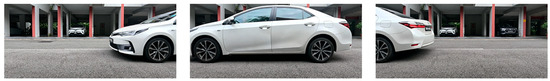
Figure 21. Estimation of vehicle speed from image frames extracted from video.

Figure 22. Speedometer readings at test run 1 and 2, respectively.

Table 10. Comparison of measured and calculated speed values.

Test Run	Distance from Car (m)	Calculated Speed (km/h)—Manual	Calculated Speed (km/h)—Image Recognition	Speedometer Reading (km/h)
1	2.28	29.5	28.3	30
2	1.92	30.9	30.0	32

6. Limitations and Future Work

The primary objective of this project was to explore the potential of available technologies like AI and machine learning to streamline and automate the process of collecting LPD of vehicles to cyclists. While we have made progress, the current setup is not entirely complete. The combination of microcontrollers and sensors employed might not be the most efficient or cost-effective, suggesting that there could be alternatives better aligned with our goals and potentially more economical. A more comprehensive testing of available commercial distance sensors would be needed to ensure that our setup remains the most cost-efficient and reliable. In addition, the current setup, which uses the Raspberry Pi, may be better off using a more space-efficient microcontroller such as the Arduino or the micro-Raspberry Pi. Moreover, the current setup relies on separated components and is not yet packaged as one. This makes the prototype less robust and portable—requiring some technical expertise from the users to properly set up. In the future, packaging the setup into one singular product would allow for easier data collection and testing on our part, but also allow for other researchers to replicate our results more easily.

Additionally, different hyperparameters or even a different clustering technique altogether could enhance our results by minimizing false positives, which requires additional testing and collection of data. Future research would consist of not only a larger volume of data collection, but also a comprehensive evaluation of different clustering algorithms across diverse datasets to affirm the universal applicability and reliability of our chosen techniques. The current data collected are only from a single path in the Jurong West region of Singapore. In future research, we would not only increase the volume of data collected, but also vary the regions that data are collected from.

Another improvement would be to fully automate the process of data extraction and analysis. Currently, we are manually extracting the data and running analysis algorithms. However, in efforts to create a standalone product for others to use, our setup might come with an application that not only collects data but analyzes and plots it for the user. Furthermore, we can fully utilize the features of the AI camera to not only filter out noise, but to also take a picture during each vehicle pass, which would provide a useful visual corresponding to the data collected. Such a feature would be well suited for a commercial product used by other researchers to assist in the collection and visualization of data.

Looking forward, the project’s evolution will encompass the assessment of a wider array of sensors, accompanied by extensive on-road data collection. These amassed data will help to test various clustering techniques, adjusting parameters to discern the optimal method. Upon establishing this foundation, our vision is to consolidate the hardware and software into a unified product kit that is readily accessible by micromobility riders.

7. Conclusions

Our research hopes to use the latest technology to advance the boundaries of transportation safety. By integrating low-cost sensors and the innovative application of data processing algorithms, we have demonstrated a robust and efficient methodology for dynamic proximity sensing of vehicles overtaking cyclists and micromobility riders. With the foundation laid by our study, subsequent research can delve deeper into optimizing data collection techniques, thereby broadening the applicability and reliability of our findings. Moreover, the existence of this research paves the way for a host of applications. Planners and policymakers can benefit from data that are more easily collected, aiding in crafting more effective transportation safety measures. Researchers can further build on this foundation by testing a broader range of sensors and algorithms, ensuring the continuous evolution and enhancement of our initial efforts. Ultimately, we hope that our research is able to work towards the goal of fostering safer roads and a more bicycle-friendly urban environment.

References

- De Hartog, J.J.; Boogaard, H.; Nijland, H.; Hoek, G. Do the Health Benefits of Cycling Outweigh the Risks? Environ. Health Perspect. 2010, 118, 1109–1116. [Google Scholar] [CrossRef] [PubMed]
- Lindsay, G.; Macmillan, A.; Woodward, A. Moving urban trips from cars to bicycles: Impact on health and emissions. Aust. N. Z. J. Public Health 2011, 35, 54–60. [Google Scholar] [CrossRef] [PubMed]
- World Health Organization. Cyclist Safety: An Information Resource for Decision-Makers and Practitioners; World Health Organization (WHO): Geneva, Switzerland, 5 November 2020; Available online: https://www.who.int/publications/i/item/cyclist-safety-an-information-resource-for-decision-makers-and-practitioners (accessed on 1 June 2023).
- Grab & Nielsen, IQ. Foods Trends Report. 2021. Available online: https://www.grab.com/sg/food/food-trends-report-2021/ (accessed on 1 June 2023).
- Singapore Police Force. Annual Traffic Statistics 2020. 2020. Available online: https://www.police.gov.sg/-/media/170D31BB17EF441881138E1A556F210C.ashx (accessed on 1 June 2023).
- Pucher, J.; Buehler, R. Cycling towards a more sustainable transport future. Transp. Rev. 2017, 37, 689–694. [Google Scholar] [CrossRef]
- Walker, I.; Garrard, I.; Jowitt, F. The influence of a bicycle commuter’s appearance on drivers’ overtaking proximities: An on-road test of bicyclist stereotypes, high-visibility clothing and safety aids in the United Kingdom. Accid. Anal. Prev. 2014, 64, 69–77. [Google Scholar] [CrossRef] [PubMed]
- Ministry of Transport. Government Accepts Recommendations from The Active Mobility Advisory Panel to Enhance Road Safety. 2019. Available online: https://www.mot.gov.sg/news/press-releases/Details/government-accepts-recommendations-from-the-active-mobility-advisory-panel-to-enhance-road-safety/ (accessed on 1 June 2023).
- von Stülpnagel, R.; Hologa, R.; Riach, N. Cars overtaking cyclists on different urban road types—Expectations about passing safety are not aligned with observed passing distances. Transp. Res. Part F Traffic Psychol. Behav. 2022, 89, 334–346. [Google Scholar] [CrossRef]
- Road Safety Authority. Examining the International Research Evidence in relation to Minimum Passing Distances for Cyclists. 2019. Available online: https://www.rsa.ie/docs/default-source/road-safety/r4.1-research-reports/safe-road-use/examining-the-international-research-evidence-in-relation-to-minimum-passing-distances-for-cyclists.pdf?sfvrsn=bf8ed37c_5 (accessed on 1 June 2023).
- Lee, O.; Rasch, A.; Schwab, A.L.; Dozza, M. Modelling cyclists’ comfort zones from obstacle avoidance manoeuvres. Accid. Anal. Prev. 2020, 144, 105609. [Google Scholar] [CrossRef] [PubMed]
- Balanovic, J.; Davison, A.; Thomas, J.; Bowie, C.; Frith, B.; Lusby, M.; Kean, R.; Schmitt, L.; Beetham, J.; Robertson, C.; et al. Investigating the Feasibility of Trialling a Minimum Overtaking Gap Law for Motorists Overtaking Cyclists in New Zealand; NZ Transport Agency Internal Report; NZ Transport Agency: Wellington, New Zealand, 2016. [Google Scholar]
- Herrera, N.; Parr, S.A.; Wolshon, B. Driver compliance and safety effects of three-foot bicycle passing laws. Transp. Res. Interdiscip. Perspect. 2020, 6, 100173. [Google Scholar] [CrossRef]
- Bella, F.; Silvestri, M. Interaction driver–bicyclist on rural roads: Effects of cross-sections and road geometric elements. Accid. Anal. Prev. 2017, 102, 191–201. [Google Scholar] [CrossRef]
- Chuang, K.H.; Hsu, C.C.; Lai, C.H.; Doong, J.L.; Jeng, M.C. The use of a quasi-naturalistic riding method to investigate bicyclists’ behaviors when motorists pass. Accid. Anal. Prev. 2013, 56, 32–41. [Google Scholar] [CrossRef] [PubMed]
- Physics Package C3FT v3.0 Product Manual; Codaxus LLC.: Austin, TX, USA, 2017.
- Feizi, A.; Mastali, M.; Van Houten, R.; Kwigizile, V.; Oh, J.S. Effects of bicycle passing distance law on drivers’ behavior. Transp. Res. Part A Policy Pract. 2021, 145, 1–16. [Google Scholar] [CrossRef]
- Schepers, P.; Theuwissen, E.; Velasco, P.N.; Niaki, M.N.; van Boggelen, O.; Daamen, W.; Hagenzieker, M. The relationship between cycle track width and the lateral position of cyclists, and implications for the required cycle track width. J. Saf. Res. 2023, 87, 38–53. [Google Scholar] [CrossRef] [PubMed]
- Mackenzie, J.; Dutschke, J.; Ponte, G. An investigation of cyclist passing distances in the Australian Capital Territory. Accid. Anal. Prev. 2021, 154, 106075. [Google Scholar] [CrossRef]
- Parkin, J.; Meyers, C. The effect of cycle lanes on the proximity between motor traffic and cycle traffic. Accid. Anal. Prev. 2010, 42, 159–165. [Google Scholar] [CrossRef] [PubMed]
- Mehta, K.; Mehran, B.; Hellinga, B. Evaluation of the Passing Behavior of Motorized Vehicles When Overtaking Bicycles on Urban Arterial Roadways. Transp. Res. Rec. J. Transp. Res. Board 2015, 2520, 8–17. [Google Scholar] [CrossRef]
- Love, D.C.; Breaud, A.; Burns, S.; Margulies, J.; Romano, M.; Lawrence, R. Is the three-foot bicycle passing law working in Baltimore, Maryland? Accid. Anal. Prev. 2012, 48, 451–456. [Google Scholar] [CrossRef] [PubMed]
- Dozza, M.; Schindler, R.; Bianchi-Piccinini, G.; Karlsson, J. How do drivers overtake cyclists? Accid. Anal. Prev. 2016, 88, 29–36. [Google Scholar] [CrossRef] [PubMed]
- Llorca, C.; Angel-Domenech, A.; Agustin-Gomez, F.; Garcia, A. Motor vehicles overtaking cyclists on two-lane rural roads: Analysis on speed and lateral clearance. Saf. Sci. 2017, 92, 302–310. [Google Scholar] [CrossRef]
- Beck, B.; Chong, D.; Olivier, J.; Perkins, M.; Tsay, A.; Rushford, A.; Li, L.; Cameron, P.; Fry, R.; Johnson, M. How much space do drivers provide when passing cyclists? Understanding the impact of motor vehicle and infrastructure characteristics on passing distance. Accid. Anal. Prev. 2019, 128, 253–260. [Google Scholar] [CrossRef]
- Mackenzie, J.; Dutschke, J.; Ponte, G. An Evaluation of Bicycle Passing Distances in the ACT (No. CASR157); Centre for Automotive Safety Research: Adelaide, Australia, 2019. [Google Scholar]
- Nolan, J.; Sinclair, J.; Savage, J. Are bicycle lanes effective? The relationship between passing distance and road characteristics. Accid. Anal. Prev. 2021, 159, 106184. [Google Scholar] [CrossRef] [PubMed]
- Ivanišević, T.; Trifunović, A.; Čičević, S.; Pešić, D.; Simović, S.; Zunjic, A.; Duplakova, D.; Duplak, J.; Manojlovic, U. Analysis and Determination of the Lateral Distance Parameters of Vehicles When Overtaking an Electric Bicycle from the Point of View of Road Safety. Appl. Sci. 2023, 13, 1621. [Google Scholar] [CrossRef]
- Yap, W. Cycling Safety Analysis [Computer Software]. Available online: https://github.com/wuihee/cycling-safety-analysis (accessed on 1 June 2023).
- Yap, W. Cycling Safety Code [Computer Software]. Available online: https://github.com/wuihee/cycling-safety-code (accessed on 1 June 2023).
- Jain, A.K.; Murty, M.N.; Flynn, P.J. Data clustering: A review. ACM Comput. Surv. 1999, 31, 264–323. [Google Scholar] [CrossRef]
- MacQueen, J. Some methods for classification and analysis of multivariate observations. In Proceedings of the Fifth Berkeley Symposium on Mathematical Statistics and Probability, Berkeley, CA, USA, 21 June–18 July 1965 and 27 December 1965–7 January 1966; Volume 1, pp. 281–297. [Google Scholar]
- Ester, M.; Kriegel, H.-P.; Sander, J.; Xu, X. A Density-Based Algorithm for Discovering Clusters in Large Spatial Databases with Noise. KDD 1996, 96, 226–231. [Google Scholar]
- Johnson, S.C. Hierarchical clustering schemes. Psychometrika 1967, 32, 241–254. [Google Scholar] [CrossRef] [PubMed]
- Reynolds, D. Gaussian Mixture Models. Encycl. Biom. 2009, 741, 659–663. [Google Scholar]
- Cheng, Y. Mean Shift, Mode Seeking, and Clustering. IEEE Trans. Pattern Anal. Mach. Intell. 1995, 17, 790–799. [Google Scholar] [CrossRef]
Disclaimer/Publisher’s Note: The statements, opinions and data contained in all publications are solely those of the individual author(s) and contributor(s) and not of MDPI and/or the editor(s). MDPI and/or the editor(s) disclaim responsibility for any injury to people or property resulting from any ideas, methods, instructions or products referred to in the content. |
© 2024 by the authors. Licensee MDPI, Basel, Switzerland. This article is an open access article distributed under the terms and conditions of the Creative Commons Attribution (CC BY) license (https://creativecommons.org/licenses/by/4.0/).