Study on the Deployment of Ultra-Wideband Positioning Base Stations in Pig Farms

Abstract

A novel indoor positioning method for a pigsty based on ultra-wideband (UWB) technology is proposed via reasonably arranging the base stations and positioning tags, which can provide strong support for the accurate positioning of specific pig pens in the pig house. The distribution of Dilution of Precision (DOP) values is analyzed in different deployment schemes which include the amount, the height, the deployment shape, and the distance of the base stations through positioning simulation. Moreover, the positioning effect of dynamic following positioning, the root-mean-square error (RMSE), and the variance of static positioning are measured. It is noteworthy that the Kalman filtering algorithm is adopted to smooth the dynamic following positioning experimental data for reducing the positioning error. The simulated results show that the DOP values decrease with the increase in height and distance, and these results and laws are consistent with the experimental results. However, the DOP values are best reached when the height is from 1.75 m to 2.75 m, and the distance is over 3.00 m. Furthermore, the DOP values of quadrilateral deployment are smaller than the ones of triangular deployment. In addition, the variance of static positioning and dynamic following positioning is decreased by utilizing the Kalman filtering algorithm. Therefore, the excellent positioning system and its solutions in a pigsty can be provided by our proposed indoor positioning method.

1. Introduction

The concept of intelligent farming has received increasing attention and research in today’s intensive, large-scale pig production environment. The use of machines over manual labor has emerged as the prevailing trend for efficient farming practices, which represents an inevitable trajectory towards the development of intelligent farming [1]. The current application of machine vision, deep learning, Internet of Things (IoT), artificial intelligence (AI), and other advanced technologies in pig farming robots has effectively freed up labor by facilitating cleaning, inspection and feeding, as well as epidemic prevention and control [2,3,4,5]. Improving production efficiency while reducing the risk of interspecies disease transmission has been demonstrated to have significant practical value and promising development prospects [6]. Navigation and positioning are the enabling technology for robots, as satellite signals cannot cover indoor pig farms. Therefore, the development of high-precision indoor positioning technology is of great importance for breeding robots.

The ultra-wideband (UWB) positioning system offers several advantages, including low system complexity, strong anti-jamming capabilities, high transmission rates, and low power consumption. It enables precise positioning and range accuracy in the decimeter or even centimeter range [7], making it suitable for the localization of breeding robots in pig farms. By deploying positioning base stations throughout the farm and equipping the robots with positioning tags, staff can accurately determine the robot’s position using a host computer. The accuracy of the tag position does not only depend on the localization algorithm, but the base station placement scheme has a great influence on the localization accuracy [8,9,10]. Some studies propose an optimization method based on the base station placement to improve the localization accuracy [11,12,13].

Dilution of Precision (DOP) is a critical parameter for evaluating positioning accuracy. It quantifies the relative geometric relationship between range error and positioning accuracy under equivalent range error conditions at the same base station. A lower DOP value indicates higher positioning accuracy [14,15]. Root-mean-square error (RMSE) measures the difference between observed and true values and is an indicator of positioning error. A smaller RMSE value indicates a smaller error and thus evaluates the position estimation accuracy of UWB indoor positioning tags [16]. Variance is used to quantify the degree of dispersion in positioning data.

By studying the principles and methods of base station deployment, this study achieves precise tag positioning by optimizing the deployment scheme, improving accuracy and stability, and providing a guarantee for high-precision positioning of breeding robots in pig farms. The paper introduces accuracy factors and their relationship with positioning accuracy, and investigates the effect of base station geometry on positioning accuracy [14,17].

A study was carried out using GDOP analysis to compare the results of mobile device positioning in different locations within a circular area with simulation results. The resolved positioning in the closed area away from the base stations, which agrees well with the simulation results, provides valuable insights for precise positioning design and testing [18]. Guo Y discovered that even if the range error is small, the localization error in a confined area is large. Therefore, a localization algorithm combining Kalman filtering (KF) and DOP is proposed to improve the accuracy and stability in such environments [19].

Albaidhani proposed a novel positioning algorithm specifically tailored for indoor applications, which was evaluated using mean-square error (MSE) and dilution of precision (DOP) as criteria to optimize base station placement and improve positioning accuracy [20]. In one study, the accuracy factor was calculated and simulated under different numbers of pseudo-satellites, and the optimal observation matrix was determined by eigenvalue analysis, with a four-satellite layout identified as optimal [21]. Based on various accuracy factors, the author proposes a four-dimensional model that includes the elevation angle, azimuth angle, and observation time as independent variables, with the relative accuracy factor as the dependent variable. This model aims to improve positioning accuracy and provide assurance for optimal satellite deployment [22]. The positioning trajectories and real trajectories of various factors were compared and analyzed through experiments, leading to the conclusion that UWB dynamic positioning is influenced by the position of positioning tags, travel speed, pedestrian interference, and the highest accuracy is in locating the center of the base station area [23]. Through real and simulated positioning experiments, this study analyzed the distribution of accuracy factors for different deployment schemes. It was concluded that the accuracy factor of test points is influenced by the regional coverage, number and height of deployed base stations, and that the accuracy of terminal positioning can be improved by increasing the number of base stations and the height angle within a closed area surrounded by base stations [24].

2. UWB Positioning Principles

The UWB positioning system used in this study utilizes the Time of Arrival (TOA) technique, which estimates the time delay from the node to be located to the reference base stations, thereby determining the distance between them. The main advantage of the TOA positioning method is its ability to exploit the high time-division rate inherent in ultra-wideband signals to accurately detect signal time delays at the receiver end, thereby allowing the distances between nodes and reference base stations to be estimated. Once these distances are estimated, the coordinates of the target node can be calculated using a basic UWB positioning algorithm. In three-dimensional space, the TOA positioning model follows a spherical representation that requires a minimum of four base stations for accurate localization. In addition, precise clock synchronization between base stations has a significant impact on positioning accuracy.

The coordinate of the jth base station is $\left(x_j,y_j,z_j\right)$. Solving for label coordinates $\left(x,y,z\right)$. Assuming the synchronization condition, i.e., no clock difference, when there are n measured values, $R_j$ represent the distance between the tag and jth base station

$$\begin{array}{c}{R}_j=\sqrt{{\left(x-x_j\right)}^2+{\left(y-y_j\right)}^2+{\left(z-z_j\right)}^2}\end{array}$$

(1)

L as a measured value which can be expressed as:

$$L=f\left(x,y,z\right)$$

According to Taylor’s theorem:

$$\begin{array}{c}L=f\left(x_0,y_0,z_0\right)+\frac{{\left(\frac{\partial L}{\partial x}\right)}_{0}dx}{1!}+\frac{{\left(\frac{\partial L}{\partial y}\right)}_{0}dy}{1!}+\frac{{\left(\frac{\partial L}{\partial z}\right)}_{0}dz}{1!}+\cdots \hfill \\ +\frac{{\left(\frac{{\partial }^{n}L}{\partial x^n}\right)}_{0}d{x}^n}{n!}+\frac{{\left(\frac{{\partial }^{n}L}{\partial y^n}\right)}_{0}d{y}^n}{n!}+\frac{{\left(\frac{{\partial }^{n}L}{\partial z^n}\right)}_{0}d{z}^n}{n!}+R_n\hfill \end{array}$$

(2)

The partial derivative at $\left(x_0,y_0,z_0\right)$ is:

$$\begin{array}{c}{\left(\frac{\partial L}{\partial x}\right)}_0=\frac{-\left(x_j-x_0\right)}{\sqrt{{\left(x_0-x_j\right)}^2+{\left(y_0-y_j\right)}^2+{\left(z_0-z_j\right)}^2}}=\frac{-\left(x_j-x_0\right)}{R_{j,0}}\end{array}$$

(3)

Assume $a_{xj}=\frac{x_j-x_0}{R_{j,0}}$ as the cosine of the direction of the coordinates solved by the positioning algorithm with respect to the base stations coordinates j:

$$\begin{array}{c}f\left(x,y,z\right)-f\left(x_0,y_0,z_0\right)={\left(\frac{\partial L}{\partial x}\right)}_{0}dx+{\left(\frac{\partial L}{\partial y}\right)}_{0}dy+{\left(\frac{\partial L}{\partial z}\right)}_{0}dz\end{array}$$

(4)

$$\begin{array}{c}∆r=a_{xj}∆x+a_{yj}∆y+a_{zj}∆z\end{array}$$

(5)

where $∆x$ is the vector of offset of the true position of the tag from the positioning algorithm solver, $∆r$ is the vector offset of the true range to the range values corresponding to the linearization point.

$$\begin{array}{c}∆r=H∆x\end{array}$$

(6)

$$∆r=\left[\begin{array}{c}∆r_1\\ ∆r_2\\ \begin{array}{c}⋮\\ ∆r_n\end{array}\end{array}\right]=\left[\begin{array}{c}\begin{array}{c}\begin{array}{ccc}{a}_{x1}& a_{y1}& a_{z1}\\ a_{x2}& a_{y2}& a_{z2}\end{array}\\ \begin{array}{lll}⋮& ⋮& ⋮\end{array}\end{array}\\ \begin{array}{ccc}{a}_{xn}& a_{yn}& a_{zn}\end{array}\end{array}\right]\left[\begin{array}{c}∆x\\ ∆y\\ ∆z\end{array}\right]$$

(7)

According to the ordinary least square (OLS)

$$\begin{array}{c}∆x={\left(H^{T}H\right)}^{-1}{H}^T∆r\end{array}$$

(8)

dx is the position error, dr is the range measurement error

$$\begin{array}{c}dx={\left(H^{T}H\right)}^{-1}{H}^{T}dr\end{array}$$

(9)

The covariance of dx is:

$$\begin{array}{ll}cov\left(dx\right)& =E\left(dxd{x}^T\right)\\ & =E\left[{\left(H^{T}H\right)}^{-1}{H}^{T}drd{r}^{T}H{\left(H^{T}H\right)}^{-1}\right]\\ & ={\left(H^{T}H\right)}^{-1}{H}^{T}cov\left(dr\right)H{\left(H^{T}H\right)}^{-1}\\ & ={\left(H^{T}H\right)}^{-1}{{\sigma }_r}^2\end{array}$$

(10)

$$\begin{array}{c}cov\left(dr\right)=I{{\sigma }_r}^2\end{array}$$

(11)

In the measurements, the errors are random, independent in zero mean, and the RMS in common.

${\sigma }_r$ is the root-mean-square (RMS), the error covariance matrix is:

$$\begin{array}{c}Q={{\sigma }_r}^{2}I\end{array}$$

(12)

$$\begin{array}{c}H=\left[\begin{array}{c}\begin{array}{c}\begin{array}{ccc}{a}_{x1}& a_{y1}& a_{z1}\\ a_{x2}& a_{y2}& a_{z2}\end{array}\\ \begin{array}{lll}⋮& ⋮& ⋮\end{array}\end{array}\\ \begin{array}{ccc}{a}_{xn}& a_{yn}& a_{zn}\end{array}\end{array}\right]\end{array}$$

(13)

The matrix of weight coefficients I is:

$$\begin{array}{c}I={\left(H^{T}H\right)}^{-1}=\left[\begin{array}{ccc}{i}_{11}& i_{12}& i_{13}\\ i_{21}& i_{22}& i_{23}\\ i_{31}& i_{32}& i_{33}\end{array}\right]\end{array}$$

(14)

$$Q={{\sigma }_r}^{2}I={{\sigma }_r}^2\left[\begin{array}{ccc}{i}_{11}& i_{12}& i_{13}\\ i_{21}& i_{22}& i_{23}\\ i_{31}& i_{32}& i_{33}\end{array}\right]=\left[\begin{array}{ccc}{q}_{11}& q_{12}& q_{13}\\ q_{21}& q_{22}& q_{23}\\ q_{31}& q_{31}& q_{33}\end{array}\right]$$

(15)

3. Positioning Results Assessment

The DOP, HDOP, VDOP, PDOP are an important basis for evaluating positioning results [17,18,25,26] GDOP is defined as the ratio of the root-mean-square (RMS) position error to the RMS ranging error. Similarly, Horizontal DOP (HDOP), Vertical DOP (VDOP), and Position DOP (PDOP) can be defined.

DOP (Dilution Of Precision) defined as:

$$\begin{array}{c}DOP=\frac{{\sigma }_x}{{\sigma }_r}\end{array}$$

(16)

HDOP (Horizontal Dilution Of Precision)

$$\begin{array}{c}HDOP=\sqrt{{\left({\left(H^{T}H\right)}^{-1}\right)}_{\mathrm{1,1}}+{\left({\left(H^{T}H\right)}^{-1}\right)}_{\mathrm{2,2}}}=\sqrt{i_{11}+i_{22}}\end{array}$$

(17)

VDOP (Vertical Dilution Of Precision)

$$\begin{array}{c}VDOP=\sqrt{{\left({\left(H^{T}H\right)}^{-1}\right)}_{\mathrm{2,2}}}=\sqrt{i_{33}}\end{array}$$

(18)

PDOP (Position Dilution Of Precision)

$$\begin{array}{c}PDOP=\sqrt{{\left({\left(H^{T}H\right)}^{-1}\right)}_{\mathrm{1,1}}+{\left({\left(H^{T}H\right)}^{-1}\right)}_{\mathrm{2,2}}+{\left({\left(H^{T}H\right)}^{-1}\right)}_{\mathrm{3,3}}}=\sqrt{i_{11}+i_{22}+i_{33}}\end{array}$$

(19)

GDOP (Geometric Dilution Of Precision)

$$\begin{array}{c}GDOP={{\sigma }_r}^2\left(i_{11}+i_{22}+i_{33}\right)=q_{11}+q_{22}+q_{33}\end{array}$$

(20)

4. Experimental Analyses

To conduct a comprehensive analysis of the positioning environment in pig farms, it is generally recommended to deploy positioning base stations along the corridor or on the walls. This study proposes multiple deployment schemes for base stations and evaluates their impact on positioning results by measuring the Dilution of Precision (DOP) value through both simulation experiments and real-world tests. The height of the positioning terminal is set at 100 cm.

4.1. Simulation and Analysis

(1)

Different heights of base stations

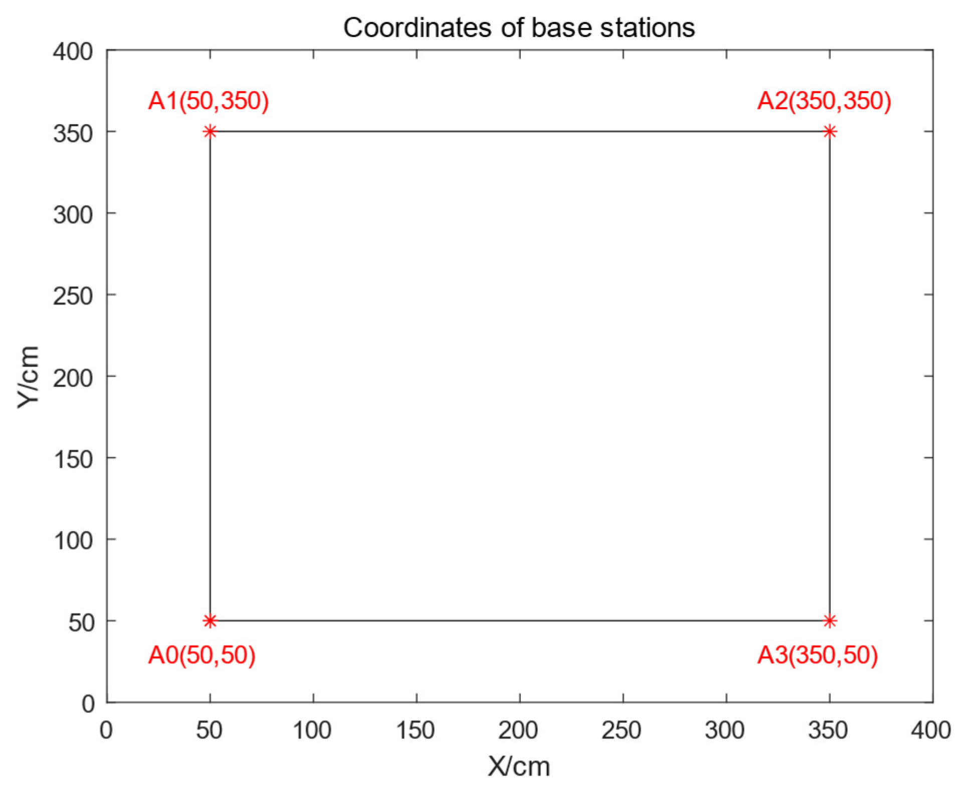
A comparative analysis is conducted to examine the impact of varying base station heights on positioning accuracy while maintaining fixed base station spacing and deployment shape conditions. The layout of the base stations is illustrated in Figure 1, wherein A₀ to A₃ represent the respective coordinate positions of each base station. The base stations are set at heights of 0 cm, 75 cm, 125 cm, 175 cm, 225 cm, and 275 cm, respectively.

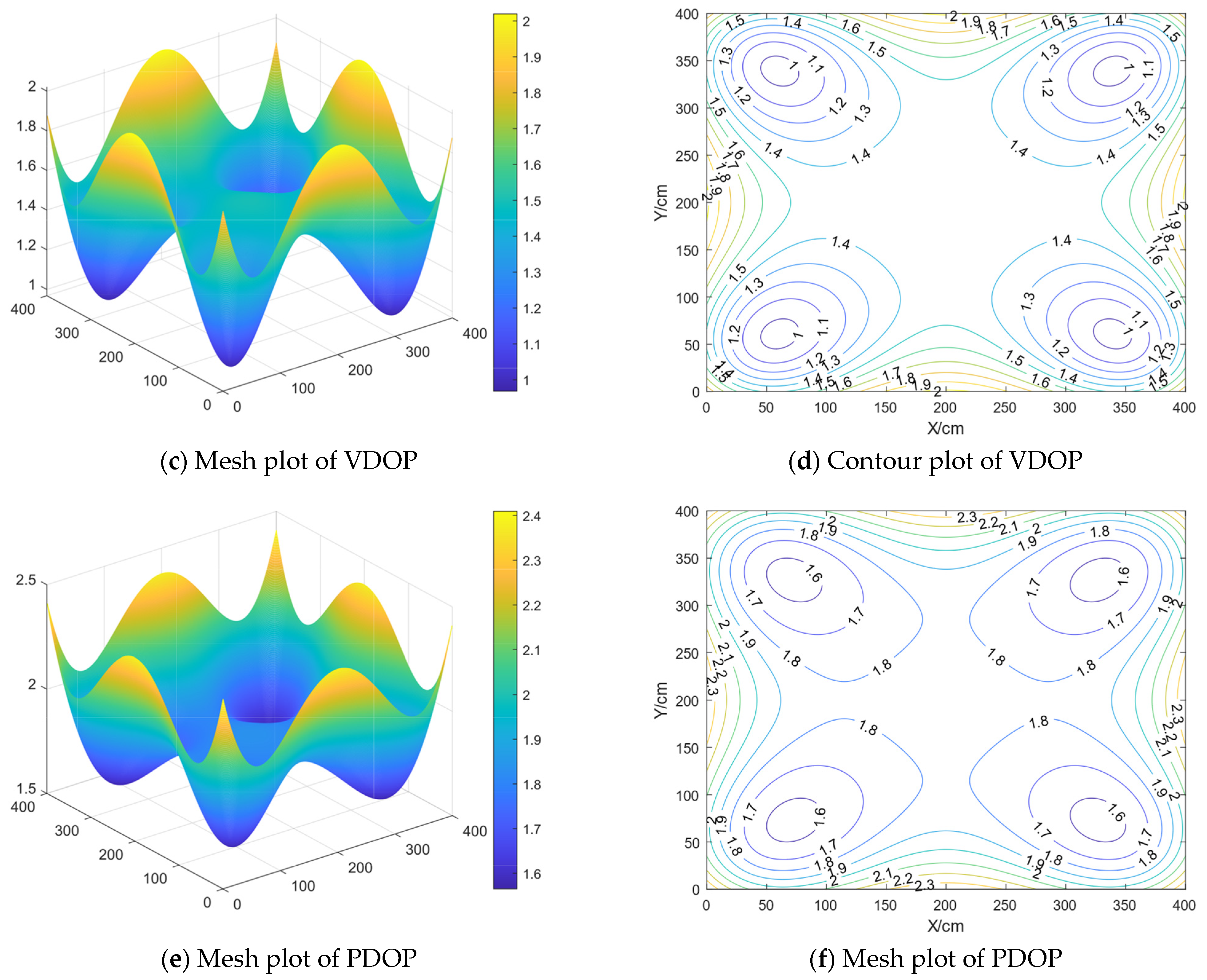
The HDOP value near the center point location is relatively smaller within the enclosed area of the base stations, as depicted in Figure 2 and supported by statistical data. Conversely, the VDOP and PDOP values tend to be larger in this region. Near the base stations, however, both VDOP and PDOP values are smaller compared to those near the center point location. Outside the closed area surrounded by the base stations, all DOP values increase with distance.

The following can be obtained through

Table 1. DOP values for simulation experiments with different heights of base stations.

DOP	Targets	a	b	c	d	e	f
HDOP	Maximum	1.55	1.47	1.47	1.51	1.60	1.72
	Minimum	1.11	1.01	1.01	1.06	1.16	1.30
	Average	1.33	1.24	1.24	1.29	1.38	1.51
VDOP	Maximum	1.62	5.58	5.58	2.02	1.49	1.35
	Minimum	0.94	1.00	1.00	0.97	0.91	0.79
	Average	1.28	3.29	3.29	1.49	1.20	1.07
PDOP	Maximum	2.25	5.71	5.71	2.41	2.18	2.19
	Minimum	1.55	1.58	1.58	1.57	1.52	1.52
	Average	1.90	3.64	3.64	1.99	1.85	1.85

Note: Scenarios a–f correspond, respectively, to heights ranging from 0 to 275 for fixed base station locations.

:

The maximum, minimum, and average DOP values of Scenarios a and b are equal to those of the other scenarios. HDOP exhibits the smallest maximum, minimum, and average values among all DOPs, while VDOP and PDOP demonstrate the largest maximum, minimum, and average values. Conversely, Scenario f exhibits the highest maximum, minimum, and average HDOP values compared to VDOP and PDOP. The differences in maximum HDOP values among scenarios do not exceed 0.3; however, there are greater disparities in maximum VDOP and PDOP values between Scenarios b and c compared to other scenarios.

In summary, given a fixed shape and spacing of the base stations’ arrangement, appropriate adjustment of the height difference between the base stations and positioning point can effectively reduce DOP values. Specifically, increasing the height of the base stations will result in larger HDOP values but smaller VDOP and PDOP values. The optimal height range for the base stations is between 175 cm and 275 cm.

(2)

Different distances of base station

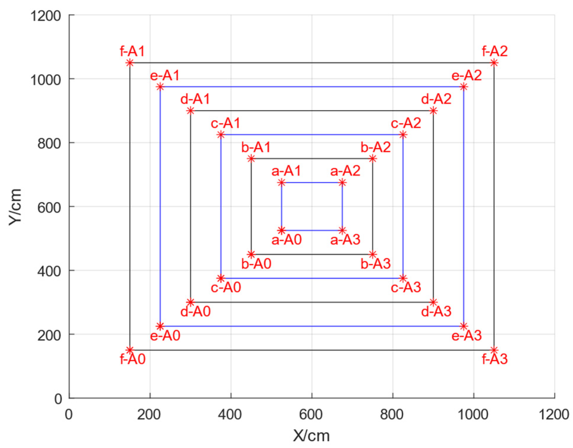
A comparative analysis was conducted to examine the impact of varying distances between base stations on positioning accuracy, considering a fixed square deployment pattern with the base station height set at 175 cm. The spacing between base station deployments were as follows: 150 cm, 300 cm, 450 cm, 600 cm, 750 cm, and 900 cm. The layout of the base stations is illustrated in Figure 3, wherein A₀ to A₃ represent the respective coordinate positions of each base station. a, b, c, d, e, f, represent scenarios with the base stations spacing of 150, 300, 450, 600, 750, and 900, respectively.

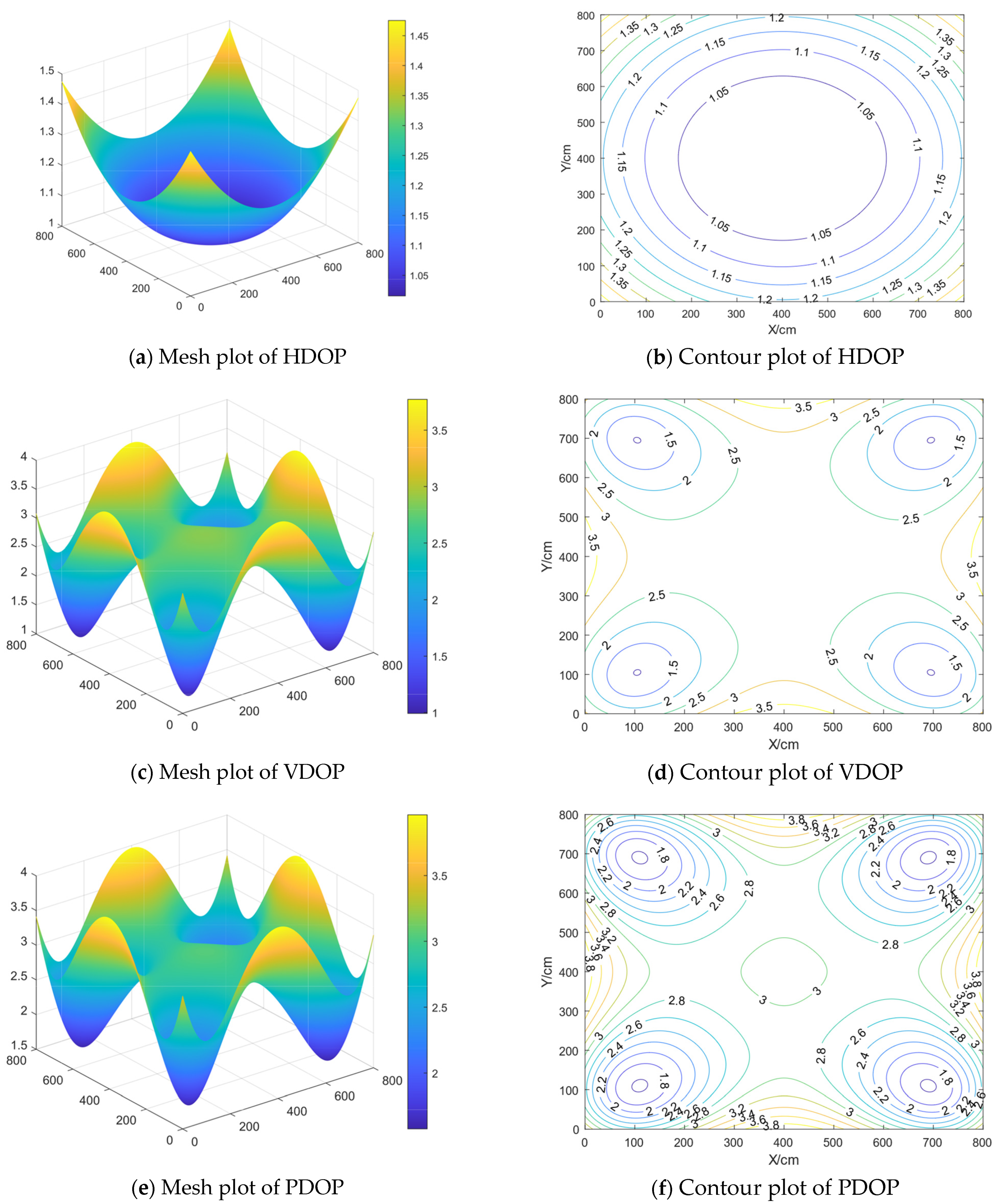
Based on Figure 4 and statistical analysis, within the square area surrounded by the base stations, Schemes b to f exhibit a smaller HDOP value as the center point gets closer, while the VDOP and PDOP values increase. As for proximity to the base stations, the VDOP and PDOP values decrease while the VDOP values increase as the center point approaches. The scheme shows that when the distance between base stations is 150 cm, all three DOP values are smaller when closer to the center. Outside of this enclosed area, the DOP values increase.

Table 2. DOP values for simulation experiments with different base station spacing.

DOP	Targets	a	b	c	d	e	f
HDOP	maximum	1.65	1.51	1.49	1.48	1.47	1.47
	minimum	1.22	1.06	1.03	1.02	1.01	1.01
	average	1.44	1.29	1.26	1.25	1.24	1.24
VDOP	maximum	1.41	2.02	2.88	3.77	4.67	5.58
	minimum	0.86	0.97	0.99	0.99	1.00	1.00
	average	1.13	1.49	1.93	2.38	2.83	3.29
PDOP	maximum	2.17	2.41	3.13	3.96	4.82	5.71
	minimum	1.50	1.57	1.57	1.58	1.58	1.58
	average	1.84	1.99	2.35	2.77	3.20	3.64

Note: Scenarios a–f correspond, respectively, distance of base stations ranging from 150 cm to 900 cm.

shows the following:

As the side length of the base stations gets bigger and bigger, the HDOP value decreases gradually, and the VDOP and PDOP values increase gradually; for Scenario f, the maximum, minimum, and average values of HDOP are the smallest, and the maximum and average values of VDOP and PDOP are the largest, but the minimum values of VDOP and PDOP for the six scenarios are basically the same.

The following summary can be obtained: when the base stations’ height and layout shape are fixed, appropriate adjustment of the base station spacing can reduce the DOP value; the larger the range of the base stations, the HDOP maximum and minimum values will be smaller; the VDOP and PDOP minimum value does not change much; the base stations’ spacing in 150 cm DOP value is relatively large; and the spacing in the range of 300 cm and above is better.

(3)

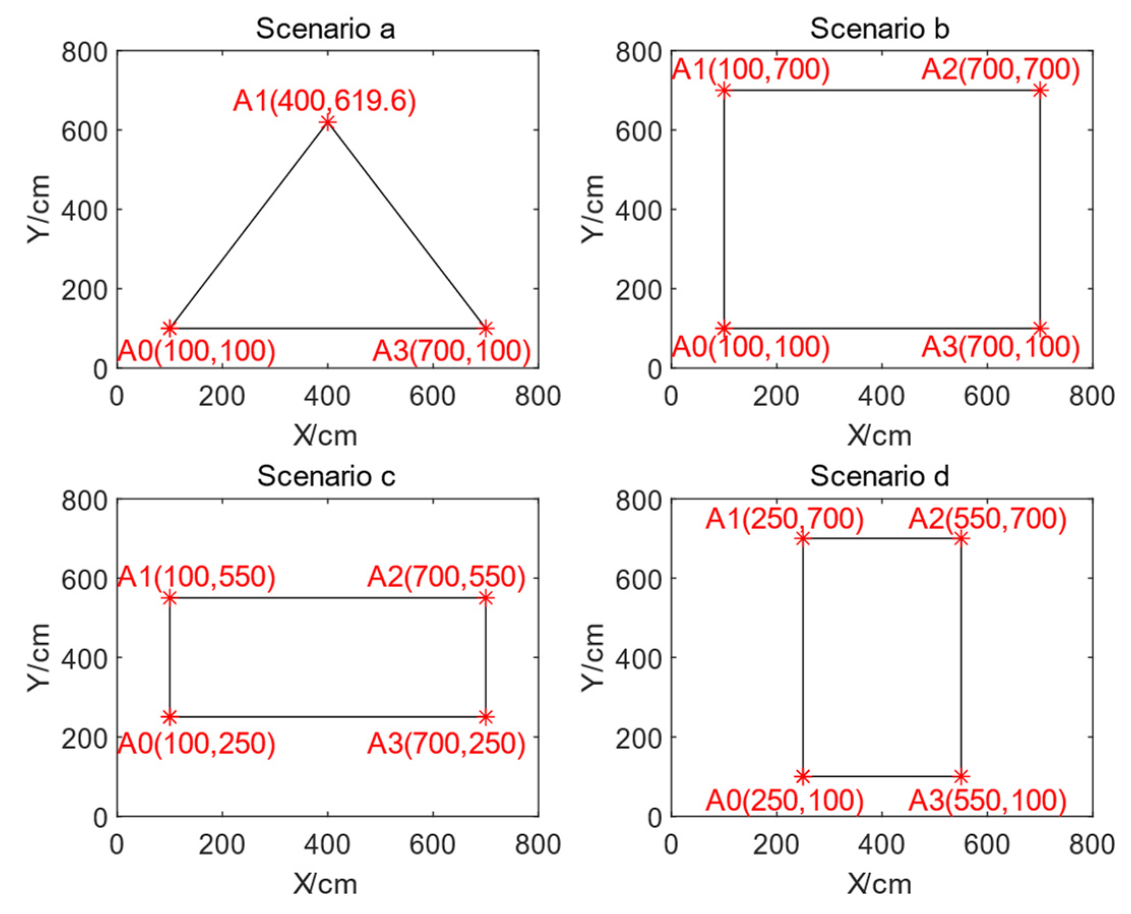
Different shapes of the base station arrangements

Comparison and analysis of the impact of different base station layouts on positioning accuracy are conducted under fixed base station spacing and height conditions. The base stations are arranged in four scenarios: an equilateral triangle with a side length of 600 cm (Scenario a), a square with a side length of 600 cm (Scenario b), a rectangle measuring 600 cm in length and 300 cm in width (Scenario c), and a rectangle measuring 300 cm in length and 600 cm in width (Scenario d). The layout and coordinates of the base stations are illustrated in Figure 5, A₀ to A₃ are the location coordinates of the base stations in the plan.

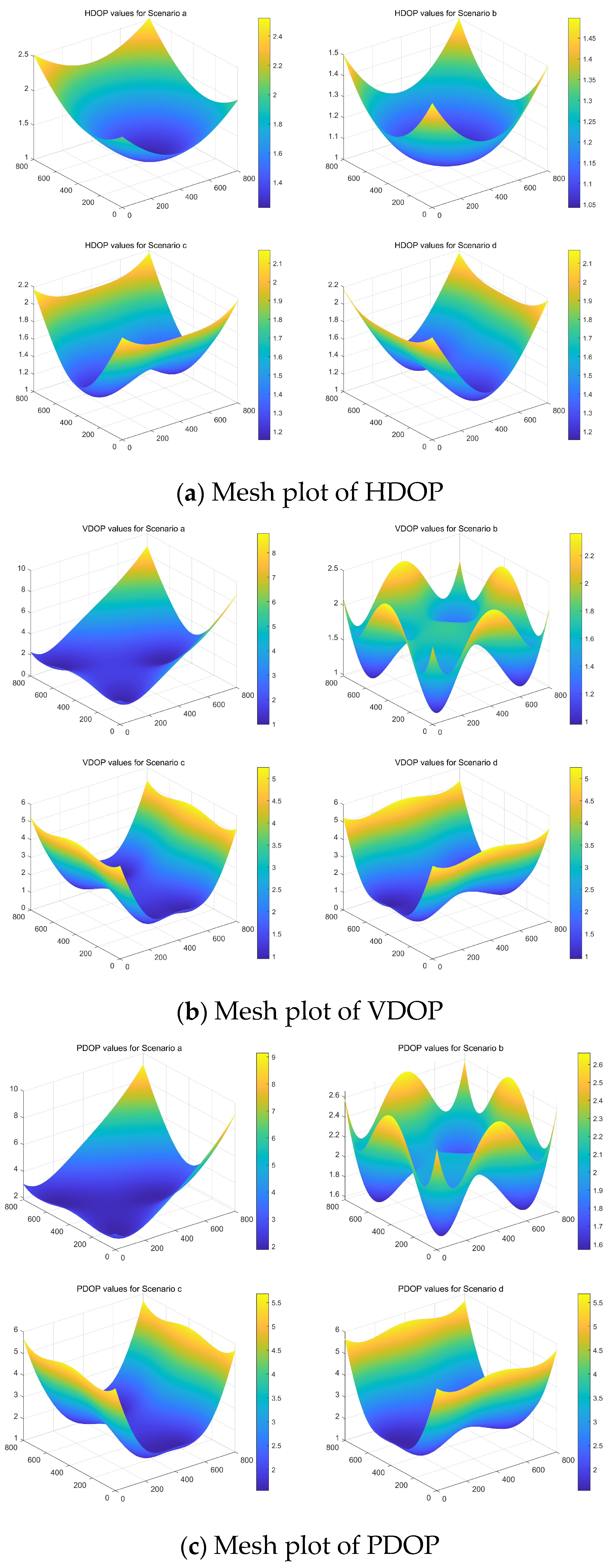
From Figure 6 the HDOP values exhibit a decreasing trend towards the central point location within the enclosed area formed by the base stations, while they increase in proximity to the base stations. Similarly, both VDOP and PDOP values are observed to decrease near the base stations. Conversely, outside this enclosed area, DOP values demonstrate an increasing pattern with greater distances from the center.

This can be obtained through

Table 3. DOP values for simulation experiments with different shapes.

DOP	Targets	Scenario a	Scenario b	Scenario c	Scenario d
HDOP	Maximum	2.50	1.48	2.13	2.13
	Minimum	1.18	1.02	1.06	1.06
	Average	1.84	1.25	1.59	1.59
VDOP	Maximum	14.47	3.77	8.47	8.47
	Minimum	0.99	0.99	0.98	0.98
	Average	7.73	2.38	4.73	4.73
PDOP	Maximum	14.69	3.96	8.69	8.69
	Minimum	1.90	1.58	1.58	1.58
	Average	8.30	2.77	5.13	5.13

:

Scenario b, when the base stations are laid out as a square, the DOP value is the smallest. In scenario a, when the equilateral triangle, the DOP value is the largest, and when the aspect ratio of rectangles is the inverse of each other, the DOP values are the same.

The conclusion can be drawn that when the base stations are deployed in a square configuration, the DOP value is minimized, resulting in optimal positioning accuracy. In comparison, deploying the base stations in a rectangular arrangement yields slightly higher DOP values for the longer side than for the shorter side, indicating relatively higher accuracy along the longer side.

4.2. Analysis of Real Measurement Experiments

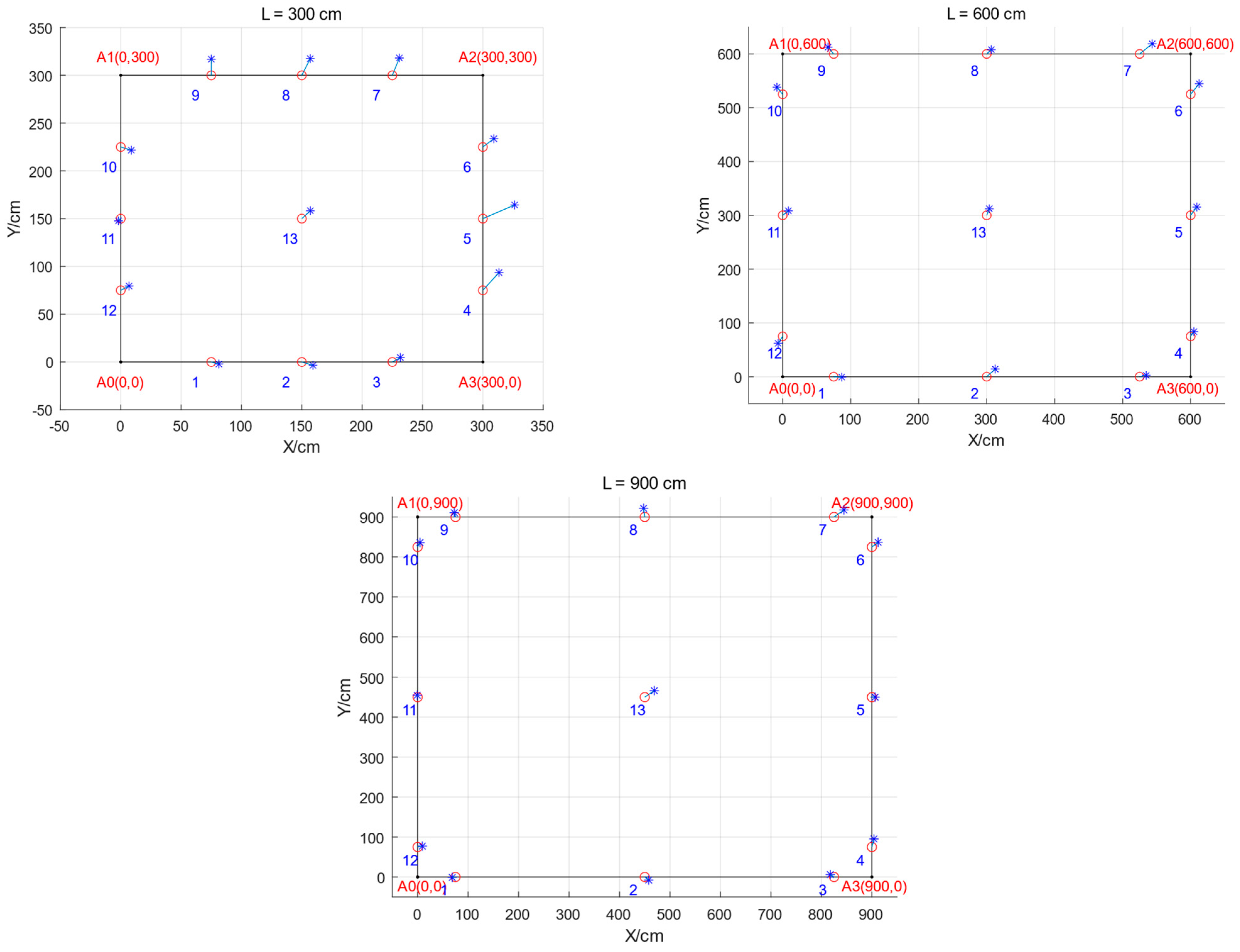
The actual measurement experiments were conducted using LinkTrack P-A module hardware, which was utilized for both static fixed-point localization and dynamic following localization in an unobstructed open field enclosed by the base stations. Additionally, the size of the test site was adjusted based on the experimental variables required.

(1)

Static positioning analysis

For the square quadrilateral area surrounded by four base stations, measurements were taken at points located approximately 75 cm from each base station, as well as at the midpoint between two adjacent base stations and the midpoint of the quadrilateral itself, resulting in a total of thirteen data points. Similarly, for the square trilateral area enclosed by three base stations, measurements were obtained near 75 cm from each base stations, at the midpoint between two adjacent base stations, and at the centroid of the triangle formed by these three stations, yielding a total of ten data points. Each fixed point was sampled within a duration of three minutes with a sampling frequency set to 10 Hz.

a.

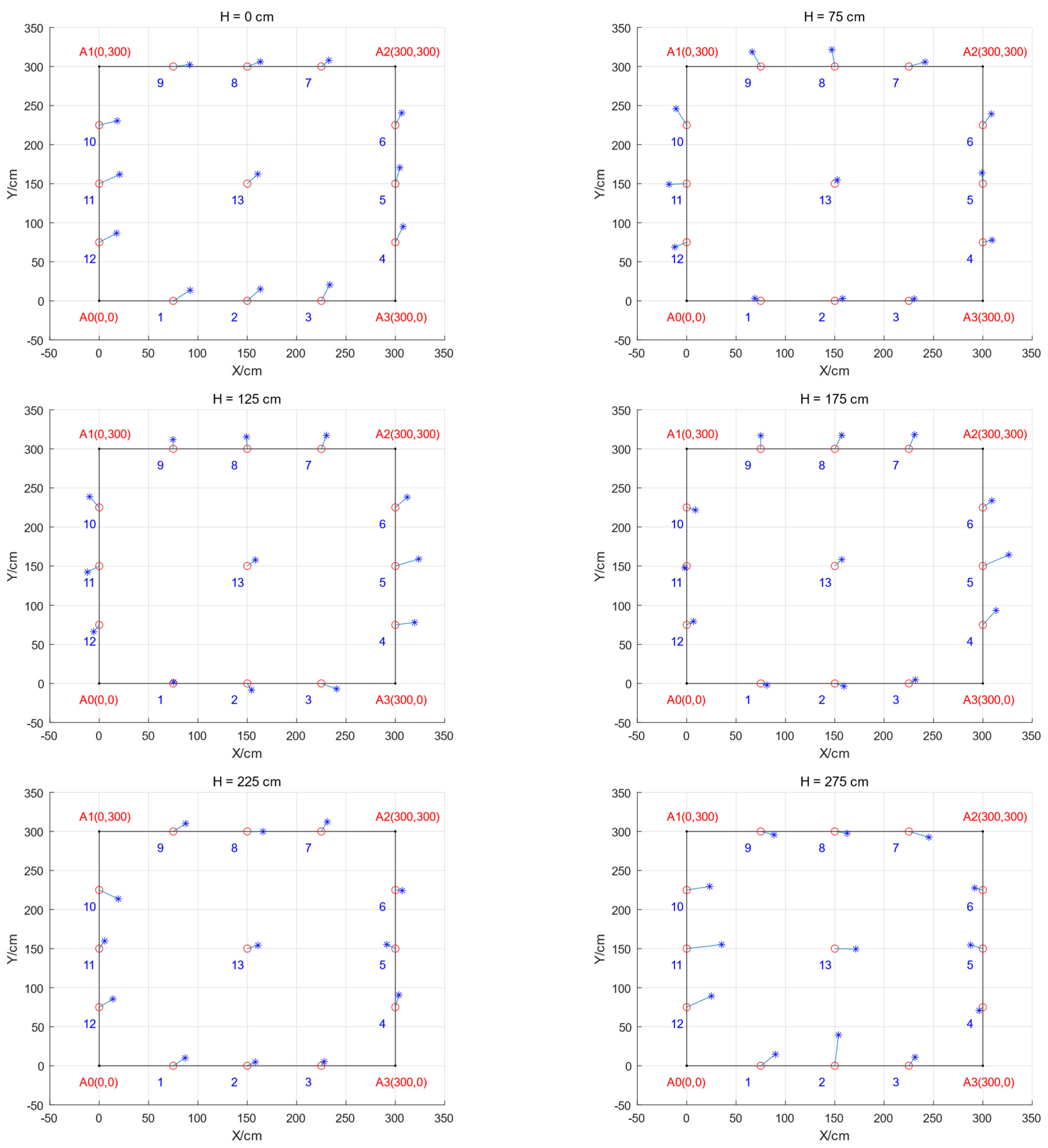
Different heights of base stations

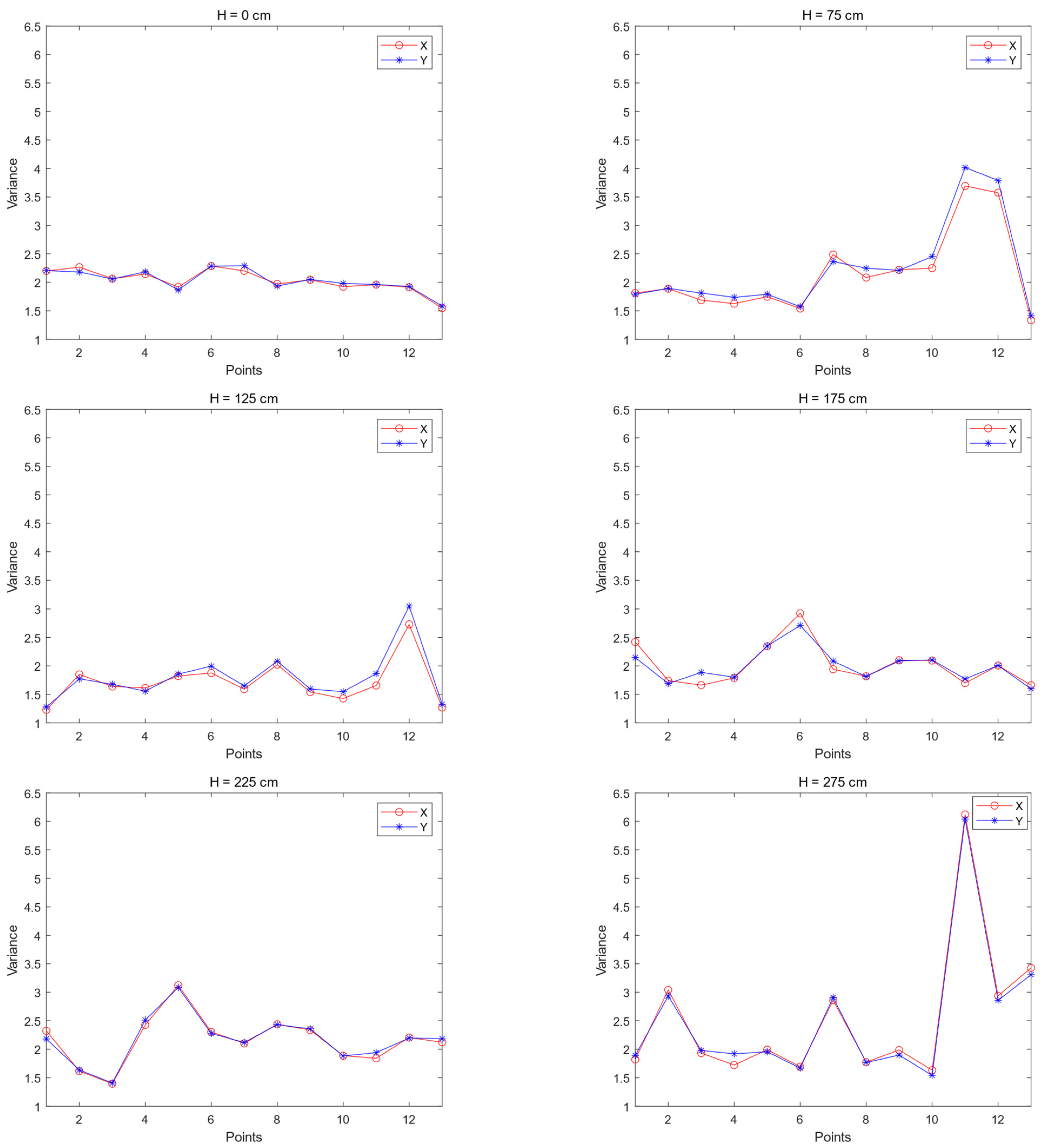
The UWB positioning effect is evaluated by enclosing the base stations in a square configuration with a spacing of 300 cm while varying the height of the base station at intervals of 0 cm, 75 cm, 125 cm, 175 cm, 225 cm, and 275 cm. The layout of the base stations are illustrated in Figure 7, wherein A₀ to A₃ represent the respective coordinate positions of each base station.

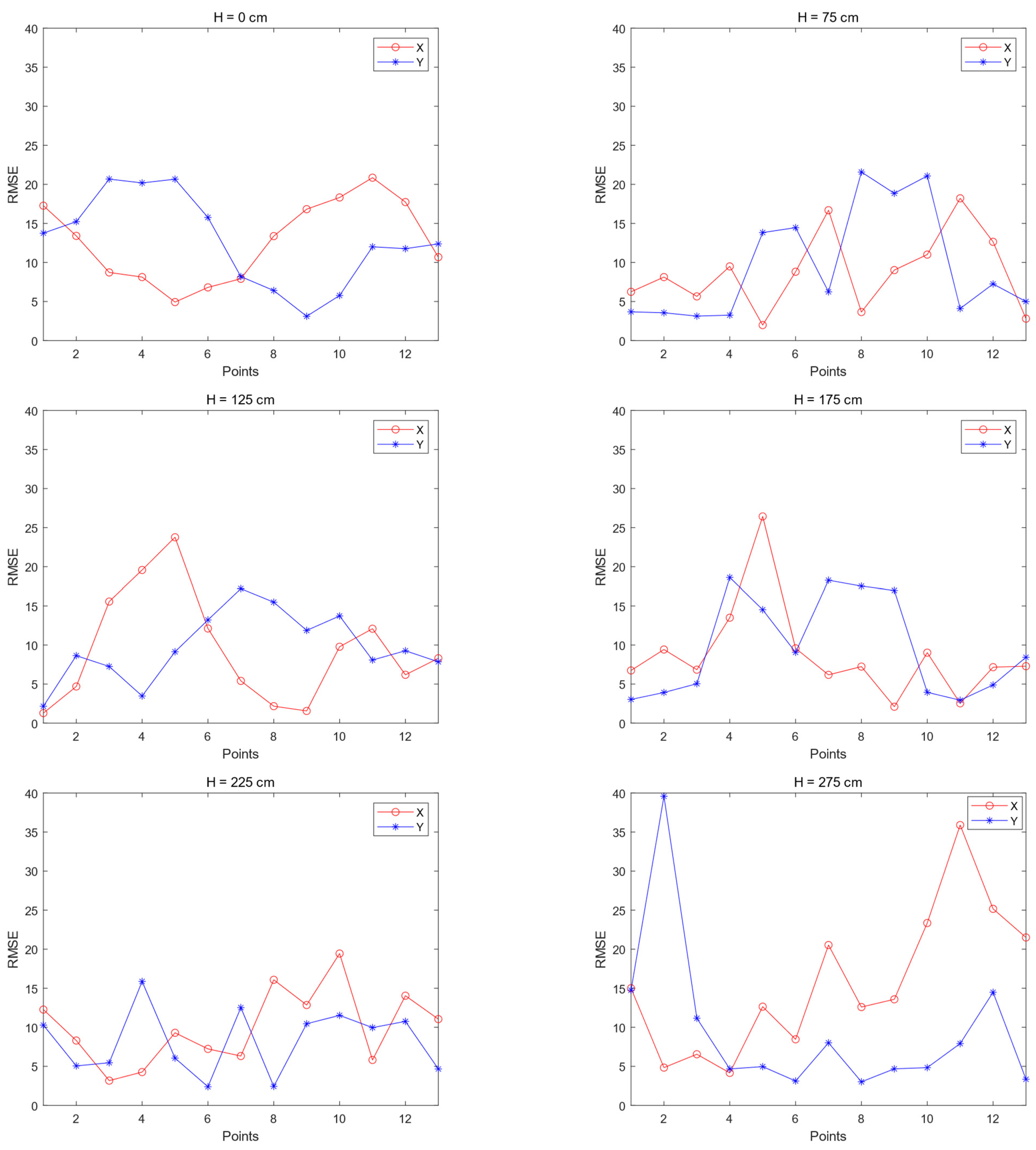
Figure 7, Figure 8 and Figure 9 show that when H is 0 cm or 275 cm, the deviation of each point is larger; when H is 175 cm or 225 cm, the deviation is smaller, and the root-mean-square error is within 15 for more points; when H is 125 cm or 175 cm, the variance is smaller for both, and within 2 for more points; when H is 275 cm, the variance is larger for more points. The same height and point location show that the X and Y coordinate variances are approximate.

Table 4. RMSE at each point with different heights of the base stations.

X/Y	RMSE Indicator	H = 0 cm	H = 75 cm	H = 125 cm	H = 175 cm	H = 225 cm	H = 275 cm
X	Maximum	20.85	18.22	23.76	26.43	19.44	35.90
	Minimum	4.93	1.98	1.28	2.10	3.17	4.16
	Average	12.89	10.10	12.52	14.27	11.31	20.03
Y	Maximum	20.68	21.58	17.20	18.62	15.87	39.59
	Minimum	3.11	3.13	2.16	2.94	2.39	3.02
	Average	11.89	12.35	9.68	10.78	9.13	21.30

shows that H is 75 cm for the X maximum value and the average value of the smallest, H is 125 cm for the X minimum value of the smallest, H is 0 cm for the X minimum value of the largest, H is 275 cm for the average value of the largest, H is 225 cm for the Y maximum value of the smallest, H is 125 cm for the Y minimum value and the average value of the smallest, H is 275 cm for the Y maximum value for the average value of the largest, and H is 0 cm for the Y minimum value of the smallest.

Table 5. Variance at points with different heights of the base stations.

X/Y	Variance Indicator	H = 0 cm	H = 75 cm	H = 125 cm	H = 175 cm	H = 225 cm	H = 275 cm
X	Maximum	2.29	3.69	2.73	2.92	3.12	6.12
	Minimum	1.55	1.34	1.23	1.66	1.39	1.63
	Average	1.92	2.51	1.98	2.29	2.26	3.88
Y	Maximum	2.29	4.02	3.05	2.71	3.08	6.04
	Minimum	1.58	1.41	1.28	1.60	1.41	1.54
	Average	1.94	2.72	2.17	2.15	2.25	3.79

shows that when H is 0 cm, X maximum value and average value are minimum; when H is 125 cm, the X minimum value is minimum; when H is 275 cm, the X maximum value and average value are maximum; when H is 175 cm, the X minimum value is maximum; when H is 0 cm, the Y maximum value and average value is minimum; when H is 125 cm, the Y minimum value is minimum; when H is 275 cm, the Y maximum value, average value is maximum and the Y minimum value is maximum. The difference between the X and Y variance values at the same point in the same height case is not significant.

b.

Different distance of base stations

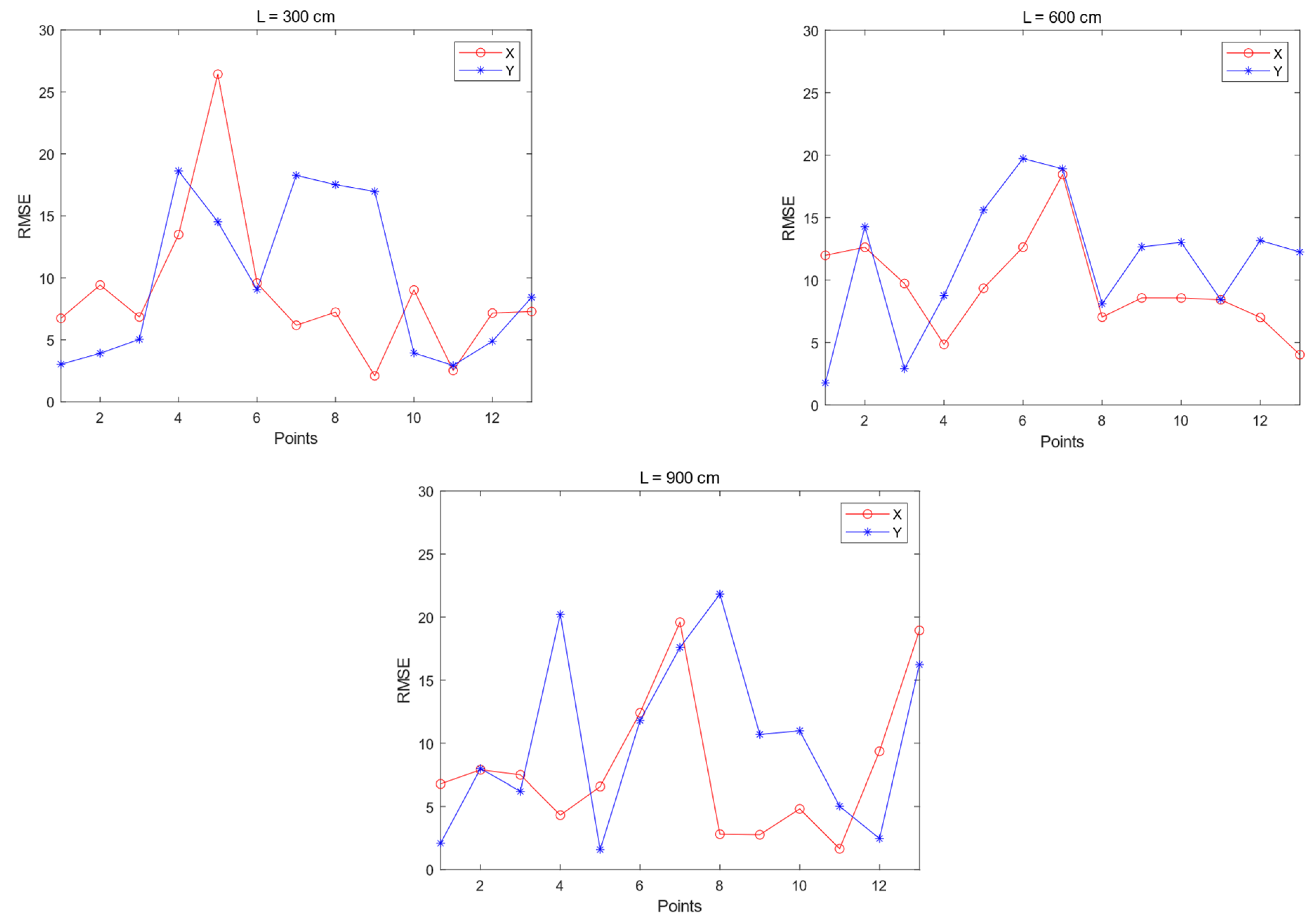
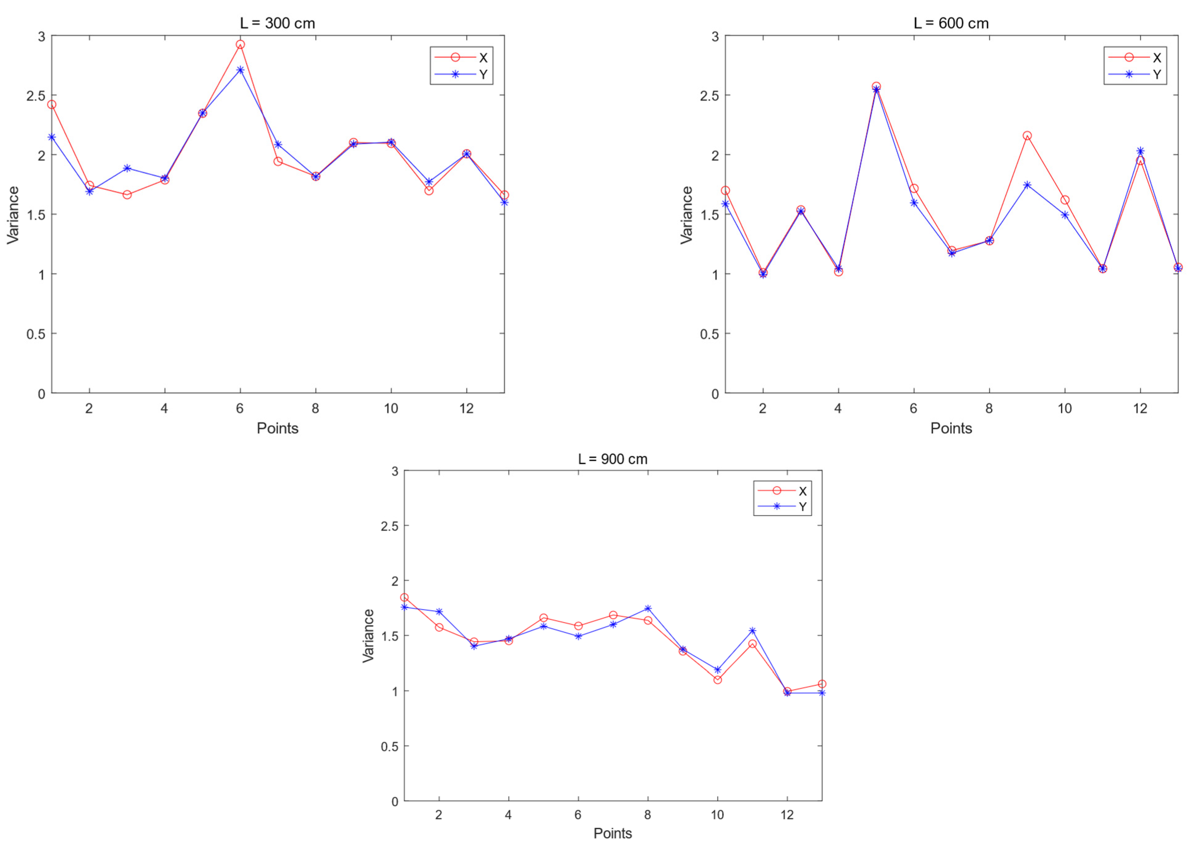
Comparison and analysis of the impact of different base station spacing on positioning accuracy is conducted in the case of a base station height of 175 cm and a fixed square deployment pattern. Due to significant fluctuations observed when deploying base stations closer together, calibration becomes impractical. Therefore, the base station deployment spacings considered are 300 cm, 600 cm, and 900 cm squares. The layout of the base stations are illustrated in Figure 10, wherein A₀ to A₃ represent the respective coordinate positions of each base station.

Figure 10, Figure 11 and Figure 12 show that there is not much difference in the root-mean-square error of each point of the three spacing cases. When L = 600 cm and 900 cm, the variance of each point is smaller, basically within 1.5; while when L = 300 cm, the variance of each point is above 1.5.

Table 6. RMSE at each point when base station spacing is different.

X/Y	RMSE Indicator	L = 300cm	L = 600cm	L = 900cm
X	Maximum	26.43	18.45	19.59
	Minimum	2.10	4.02	1.65
	Average	14.27	11.24	10.62
Y	Maximum	18.62	19.72	21.82
	Minimum	2.94	1.76	1.58
	Average	10.78	10.74	11.70

shows that when L is 600 cm, the maximum value of X is the smallest; when L is 900 cm, the minimum value of X and the average value are the smallest; when L is 300 cm, the maximum value of Y is the smallest; when L is 900 cm, the minimum value of Y is the smallest; and when L is 600 cm, the average value of Y is the smallest.

Table 7. Variance at points with different base station spacing.

X/Y	Variance Indicator	L = 300cm	L = 600cm	L = 900cm
X	Maximum	2.92	2.57	1.85
	Minimum	1.66	1.01	1.00
	Average	2.29	1.79	1.42
Y	Maximum	2.71	2.55	1.76
	Minimum	1.60	0.99	0.98
	Average	2.15	1.77	1.37

shows that when L is 900 cm, the X and Y maximum and minimum and average values are the smallest; with the same spacing, the X and Y variance value of the same point does not differ much. The larger the spacing, the smaller the variance, that is, the more stable the positioning.

c.

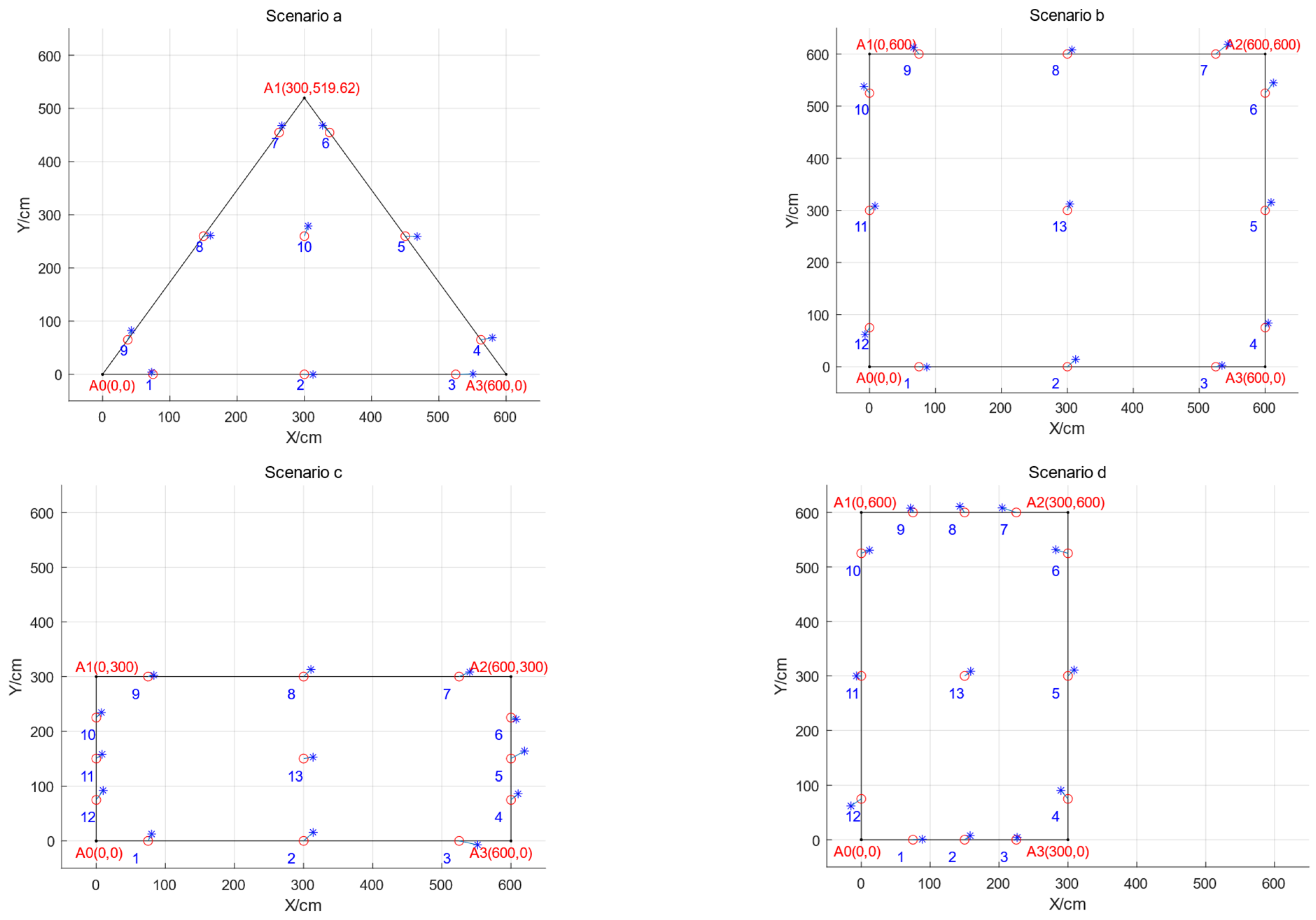
Different shapes of base station arrangements

After comparison and analysis of the effect of different shapes of base station layout on positioning accuracy in the case of fixed base station spacing and base station height, the base station layout is set up as an equilateral triangle with a side length of 600 cm (Scenario a), a square with a side length of 600 cm (Scenario b), a rectangle with a length of 600 cm and a width of 300 cm (Scenario c), and a rectangle with a length of 300 cm and a width of 600 cm (Scenario d), respectively. The layout of the base stations are illustrated in Figure 13, wherein A₀ to A₃ represent the respective coordinate positions of each base station.

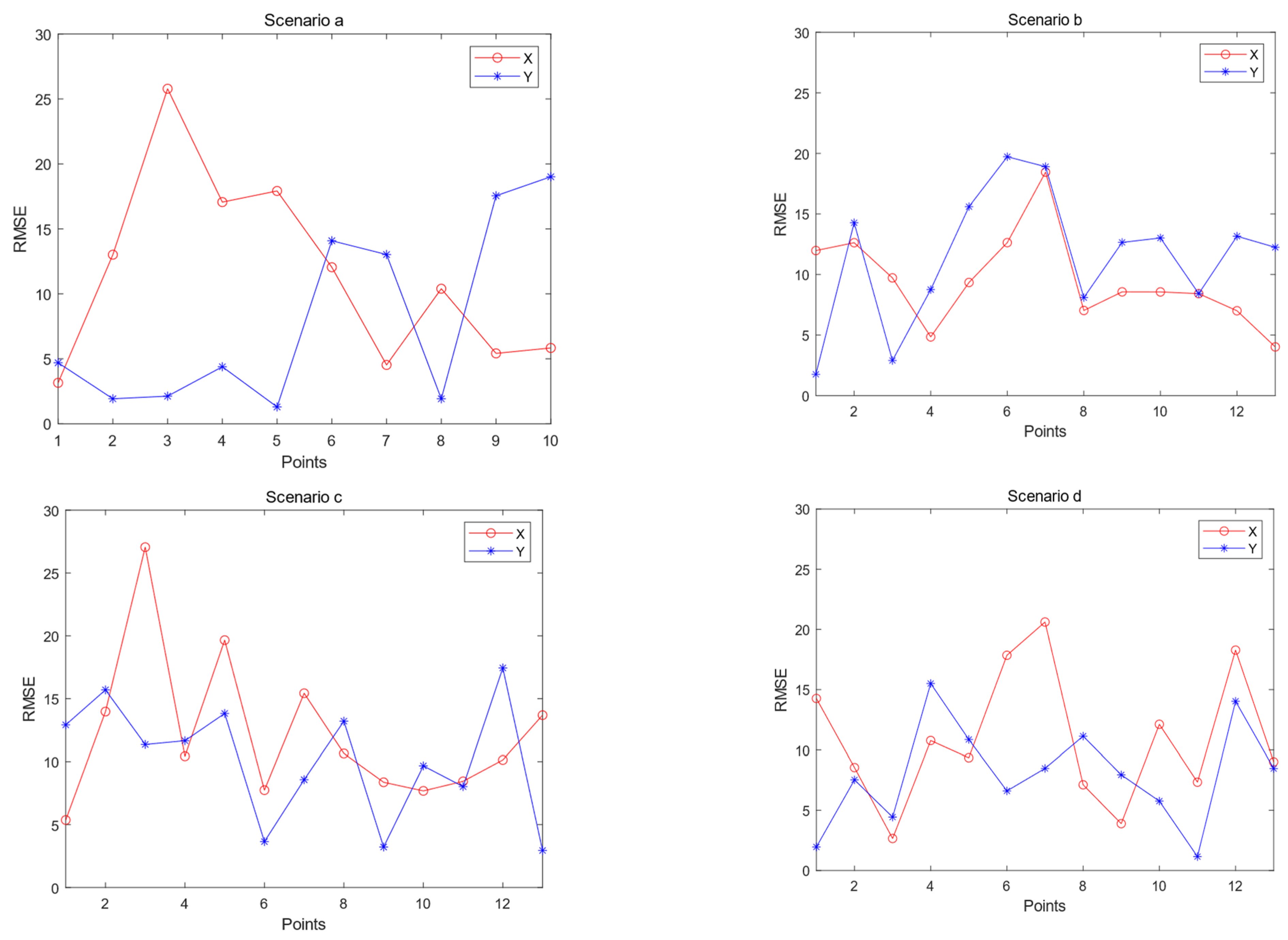
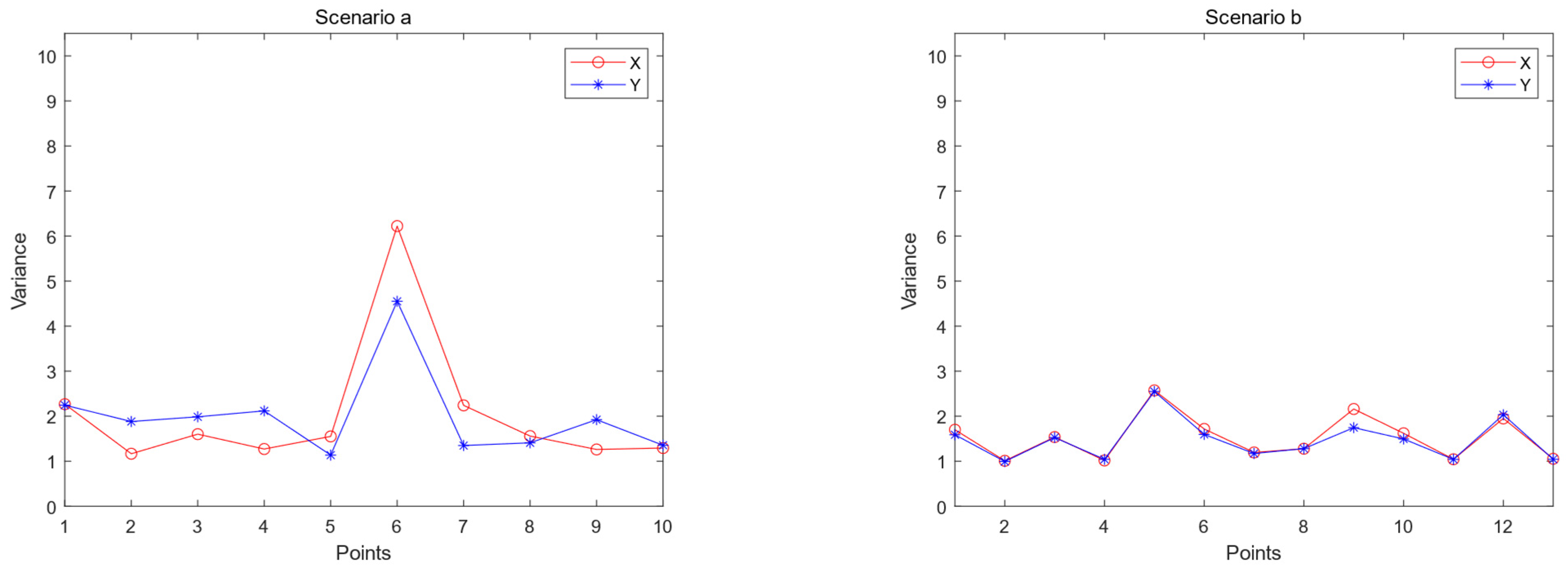
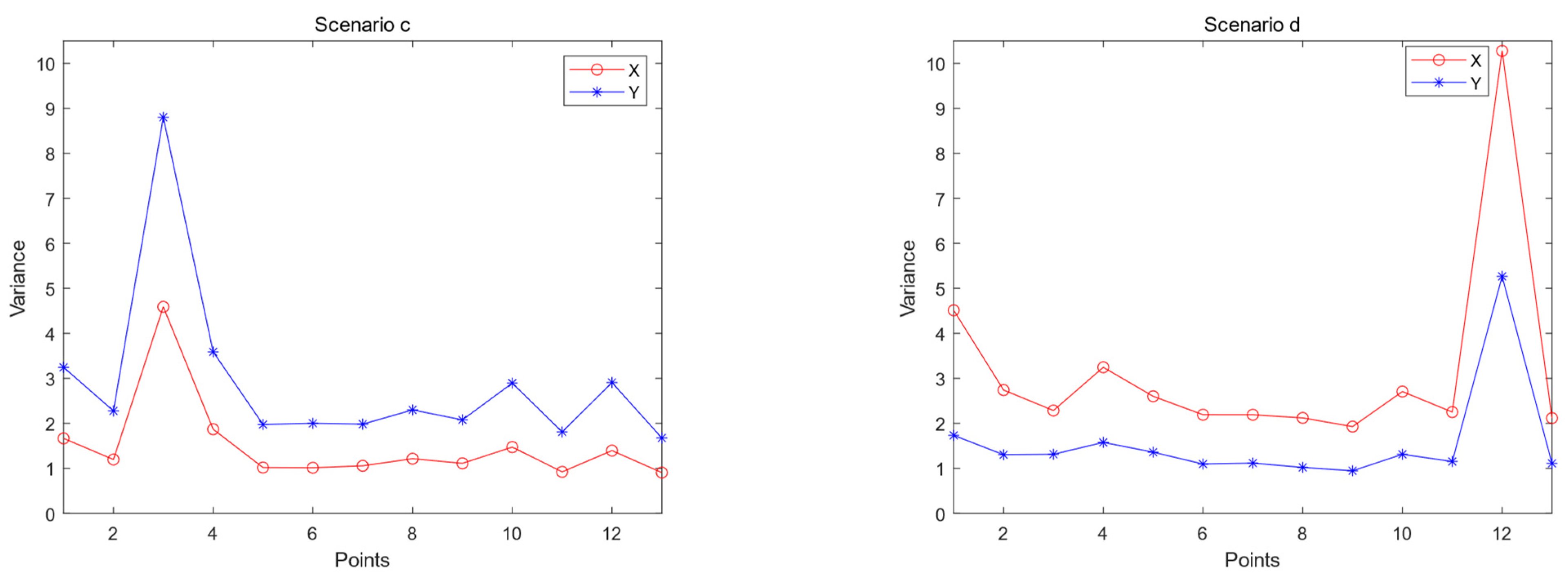
The results depicted In Figure 13, Figure 14 and Figure 15 demonstrate that when the base stations are arranged in a square configuration, the majority of points exhibit a root-mean-square error below 15, with X and Y variances exhibiting close proximity and minimal values. Conversely, when the base stations are arranged as a triangle or rectangle, individual points display significantly larger root-mean-square errors and variances. Specifically, for rectangular configurations where the width exceeds the length, the X variance of identical points is smaller than their corresponding Y variance, whereas for rectangles where the length surpasses the width, the Y variance of identical points is smaller than their corresponding X variance.

Table 8. RMSE at each point when the shape of the base station deployment is different.

X/Y	RMSE Indicator	Scenario a	Scenario b	Scenario c	Scenario d
X	Maximum	25.78	18.45	27.05	20.62
	Minimum	3.15	4.02	5.37	2.66
	Average	14.47	11.24	16.21	11.64
Y	Maximum	19.01	19.72	17.44	15.51
	Minimum	1.30	1.76	2.94	1.16
	Average	10.15	10.74	10.19	8.33

shows that the X maximum, minimum, and mean of Scenario c are all the largest, the X maximum and mean of the square are all the smallest, and the X minimum of Scenario d is the smallest; the maximum and mean of Y of Scenario b are all the largest, and the Y maximum, minimum and mean of Scenario c are all the smallest.

Table 9. Variance at points with different shapes of base station deployment.

X/Y	Variance Indicator	Scenario a	Scenario b	Scenario c	Scenario d
X	Maximum	6.22	2.57	4.59	10.28
	Minimum	1.17	1.01	0.91	1.93
	Average	3.69	1.79	2.75	6.10
Y	Maximum	4.55	2.55	8.80	5.27
	Minimum	1.14	0.99	1.68	0.95
	Average	2.84	1.77	5.24	3.11

shows that the maximum, minimum, and mean values of X and Y are minimum for Scenario b; the maximum, minimum, and mean values of X are maximum for Scenario d; and the maximum, minimum, and mean values of Y are minimum for Scenario c.

(2)

Dynamic positioning analysis

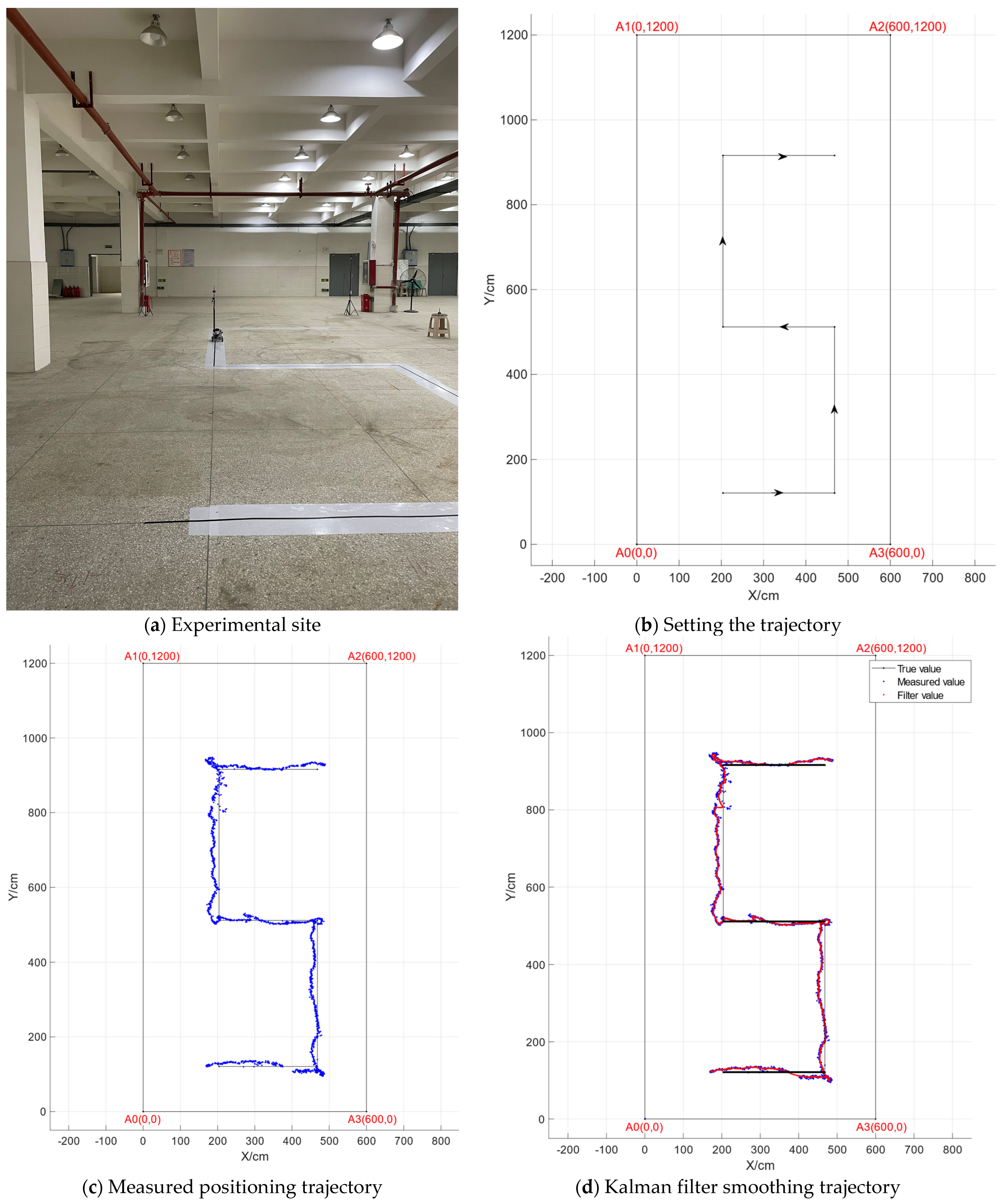
Dynamic experimental site selection was conducted in the 6 m × 12 cm open hall, following a predetermined path. Four UWB modules were used as base stations, fixed at a height of 175 cm. A UWB module was attached to a bracket rod and secured to the machine trolley, positioning it at a fixed distance of 1m from the ground. The trolley was operated remotely using a set path for dynamic positioning tests. The positioning system operated at a frequency of 10 Hz, with NAssistant V1.0 software on the host PC supporting UWB positioning. The machine car is the ROS machine car of WHEELTEC, controlled by Jetson TX1. Positioning data was recorded and saved, as depicted in Figure 16.

The observation from Figure 16 reveals that the vertical coordinate offset in UWB following positioning is relatively small, while the horizontal coordinate offset is significant. Moreover, the positioning effect is more favorable when the trajectory moves horizontally rather than vertically. It should be noted that UWB positioning involves discrete points, and employing Kalman filtering can effectively smooth and correct these discrete positioning points.

5. Conclusions

The UWB positioning effect in different deployment environments is investigated through MATLAB R2021a simulation positioning experiments and UWB measurement experiments. The impact of base stations’ deployment height, distance between base stations, and shape of the base station deployment on the UWB positioning effect is analyzed. Additionally, the effects of base station deployment on the DOP value and positioning error are simulated and analyzed. Static measurement experiments further analyze the effects of base station deployment on each point location’s positioning effect, as well as variance and root-mean-square error. Based on these analyses, the following conclusions can be drawn:

(1)

In the simulation experiment, within the enclosed area surrounded by base stations, there is an inverse relationship between proximity to the center and HDOP value, as well as proximity to the base stations and VDOP/PDOP values. Moreover, VDOP and PDOP values within this closed area are smaller than the average. Conversely, outside of this enclosed area, DOP values increase with distance from the center. The optimal height range for base stations is determined to be between 175 cm and 275 cm. Additionally, a spacing of more than 300 cm between base stations yields better positioning accuracy. When arranging base stations in a square formation, superior positioning results can be achieved compared to a rectangular layout where longer sides exhibit better performance than shorter sides.

(2)

In the actual experiment, when the base stations are arranged in a square configuration with a side length of 300 cm, adjusting the height of the base stations has an impact on the positioning accuracy. Specifically, at heights of 0 cm and 275 cm, there is significant and fluctuating positioning deviation observed. However, optimal results are achieved when the height of the base stations ranges from 175 cm to 225 cm.

(3)

When the base stations are arranged in a square configuration with a height of 175 cm, the positioning effect can be influenced by adjusting the spacing between base stations. Smaller spacing leads to significantly larger root-mean-square errors at individual points; when the spacing is less than 300 cm, there is a calibration deviation of more than 100 cm within the base stations themselves, resulting in calibration failure and inaccurate positioning. Spacing equal to or greater than 300 cm provides a wider UWB accuracy range, with increased stability in positioning as spacing increases.

(4)

When the base stations are deployed in a triangular, square, and rectangular configuration with a height of 175 cm and a spacing of 600 cm, the variance of the X and Y coordinates is consistently smaller for the square configuration, indicating superior stability in positioning. Conversely, both the triangular and rectangular configurations exhibit larger deviations among individual points. Furthermore, when deployed as a rectangle, it is observed that longer sides yield better positioning accuracy compared to shorter sides.

(5)

The deviation of the midpoint within the closed graph of the base station deployment is minimized, resulting in an enhanced positioning effect.

(6)

During the positioning process, the UWB system generates discrete coordinate points in the host computer software, which can be further optimized using a Kalman filter to refine the trajectory.

(7)

The results of the two experiments demonstrate that the positioning accuracy can be enhanced and optimized by adjusting the vertical deployment height, inter-base station spacing, and geometric configuration of base stations.

In conclusion:

Different heights of the base stations: the appropriate height is between 175 cm and 225 cm.

Different distance of the base stations: spacing in the range of 300 cm and above is better.

Different shape of the base station arrangements: when the base stations are deployed as a square, the DOP is the smallest and the positioning effect is the best.

In the practical application scenario, the deployment of base stations is constrained by environmental limitations and inevitably influenced by various factors such as multipath effects, non-line-of-sight propagation, and interference from multiple sites. These factors can lead to significant deviations in positioning accuracy. Therefore, the subsequent experiment aims to investigate the impact of each interfering object within the farm on positioning accuracy based on specific deployments and establish a low-impact deployment model to enhance farm positioning precision.