Short-Term Wind Power Prediction Based on Feature-Weighted and Combined Models

Abstract

Accurate wind power prediction helps to fully utilize wind energy and improve the stability of the power grid. However, existing studies mostly analyze key wind power-related features equally without distinguishing the importance of different features. In addition, single models have limitations in fully extracting input feature information and capturing the time-dependent relationships of feature sequences, posing significant challenges to wind power prediction. To solve these problems, this paper presents a wind power forecasting approach that combines feature weighting and a combination model. Firstly, we use the attention mechanism to learn the weights of different input features, highlighting the more important features. Secondly, a Multi-Convolutional Neural Network (MCNN) with different convolutional kernels is employed to extract feature information comprehensively. Next, the extracted feature information is input into a Stacked BiLSTM (SBiLSTM) network to capture the temporal dependencies of the feature sequence. Finally, the prediction results are obtained. This article conducted four comparative experiments using measured data from wind farms. The experimental results demonstrate that the model has significant advantages; compared to the CNN-BiLSTM model, the mean absolute error, mean squared error, and root mean squared error of multi-step prediction at different prediction time resolutions are reduced by $35.59\%$, $59.84\%$, and $36.77\%$ on average, respectively, and the coefficient of determination is increased by $1.35\%$ on average.

1. Introduction

The depletion of traditional fossil fuels and the resulting pollution are making energy supply and improvement increasingly severe. Currently, wind power as a non-polluting and sustainable new energy has received widespread attention [1]. Renewable energy, represented by wind power, holds immense significance in addressing energy depletion and improving the energy structure. However, wind power is subject to variability and intermittency, which poses a challenge to grid stability when large-scale wind power integration takes place [2]. Accurate wind power forecasting is one such crucial solution that enhances the reliability and efficiency of power systems [3,4,5]. At the same time, it provides guidance for grid scheduling plans and maintains balance in wind power supply and demand [6,7].

Wind power forecasting can be categorized into ultra-short-term, short-term, medium-term, and long-term forecasts based on the time horizon [8]. The ultra-short-term range is a few minutes (0–30 min), which can aid power system operators in real-time scheduling and the optimization of generation [9]. The short-term prediction range is from hours to days (hours–days), mainly used for market trading and the optimization scheduling of wind farms [10]. The medium and long-term predictions range from days to weeks, which can provide assistance and guidance for long-term maintenance planning and the energy management of wind farms [11]. Considering the stability and the economy of the power system, short-term wind power forecasting has become the focus of research.

Physical models, statistical models, artificial intelligence models, and composite models are four commonly used methods [12]. Numerical weather prediction (NWP) is one of the most widely used physical models. It is based on physical equations and utilizes information about the surrounding physical environment to establish a prediction model [13]. This type of method does not require historical wind power data but is computationally complex [14]. Statistical models predict future wind power output by analyzing patterns and trends in historical data. The advantage of statistical models is their low computational cost. Traditional statistical models include the autoregressive moving average (ARMA) model [15] and the autoregressive integrated moving average (ARIMA) model [16]. The above statistical model assumes that the relationship between time series data is linear in advance, which cannot deal with the nonlinear characteristics of wind power series [17].

Artificial intelligence models exhibit remarkable nonlinear fitting capabilities when processing data and have been widely used in wind power prediction [18]. For example, artificial neural networks (ANNs) [19] and support vector machines (SVMs) [20] combined with optimization algorithms have been applied to short-term wind power forecasting, and these methods have been shown to exhibit excellent predictive performance. Deep learning, as a class of artificial intelligence methods, can learn more complex non-linear relationships, thus being highly favored in wind power forecasting [21]. For instance, recurrent neural networks (RNNs) can effectively process sequential data and produce good predictive results. However, considering that RNNs often faces the problems of vanishing or exploding gradients, variants of RNNs are mainly used, such as long short-term memory (LSTM) networks [22] or gated recurrent unit (GRU) networks [23]. Convolutional Neural Networks (CNNs) leverage unique convolution operations to effectively extract high-level features from wind power time series data, leading to accurate prediction results [24]. Nevertheless, these prediction models still have limitations. LSTM can only extract forward time information from the input and ignore backward time information [25]. Graves et al. [26] proposed BiLSTM, a model that can simultaneously consider bidirectional information and achieves better predictive accuracy than LSTM. Commonly used CNNs have only one type of convolutional kernel, limiting their ability to capture hidden features of different scales when processing multivariate wind power data [27]. To accurately predict wind power, the use of CNNs with multiple convolutional kernels has become urgently needed [28]. However, CNNs still struggle to capture long-term trends in time series. Therefore, the prediction results using only a single model are not satisfactory.

The combined models can leverage the strengths of diverse models and have strong adaptive abilities when dealing with non-stationary signals [29,30]. A prediction method of CNN-LSTM was proposed in reference [31]. It was demonstrated that the prediction performance of the CNN-LSTM model exceeded that of either a standalone CNN or LSTM. Zhou et al. [32] combine LSTM and the K-Means clustering algorithm with the non-parametric kernel density estimation (KDE) method to improve prediction accuracy. The forecasting method described above uses the long-term trends of the raw data, which are messy, and with an increasing prediction time range, information loss is likely to occur, thus affecting the prediction performance. One way to tackle this challenge is to decompose the wind power data for the better learning of its structural and characteristic patterns by models. Lu et al. [33] use variational mode decomposition and weighted permutation entropy (VMD-WPE) decomposition of historical wind power and key meteorological features as inputs to build a CNN-LSTM model and use different optimizers to seek out the best parameters for the model, with the aim of achieving accurate prediction outcomes. However, this two-stage decomposition method increases the complexity of data processing, and the sensitivity of VMD to noise can also affect the prediction results. In addition, analyzing only key meteorological features equally without considering the differences in the impact of various meteorological features on wind power output will also reduce the accuracy of the forecast. Another method to improve prediction accuracy is to add an attention mechanism to the model. Tang et al. [34] proposed a CNN-LSTM-Attention prediction method, which weights the output of CNN-LSTM with attention to make the model focus more on the important features for prediction results, reduce information loss, and improve prediction accuracy. However, this way of introducing the attention mechanism requires the combined models to have a high ability to extract features and their long-term trends.

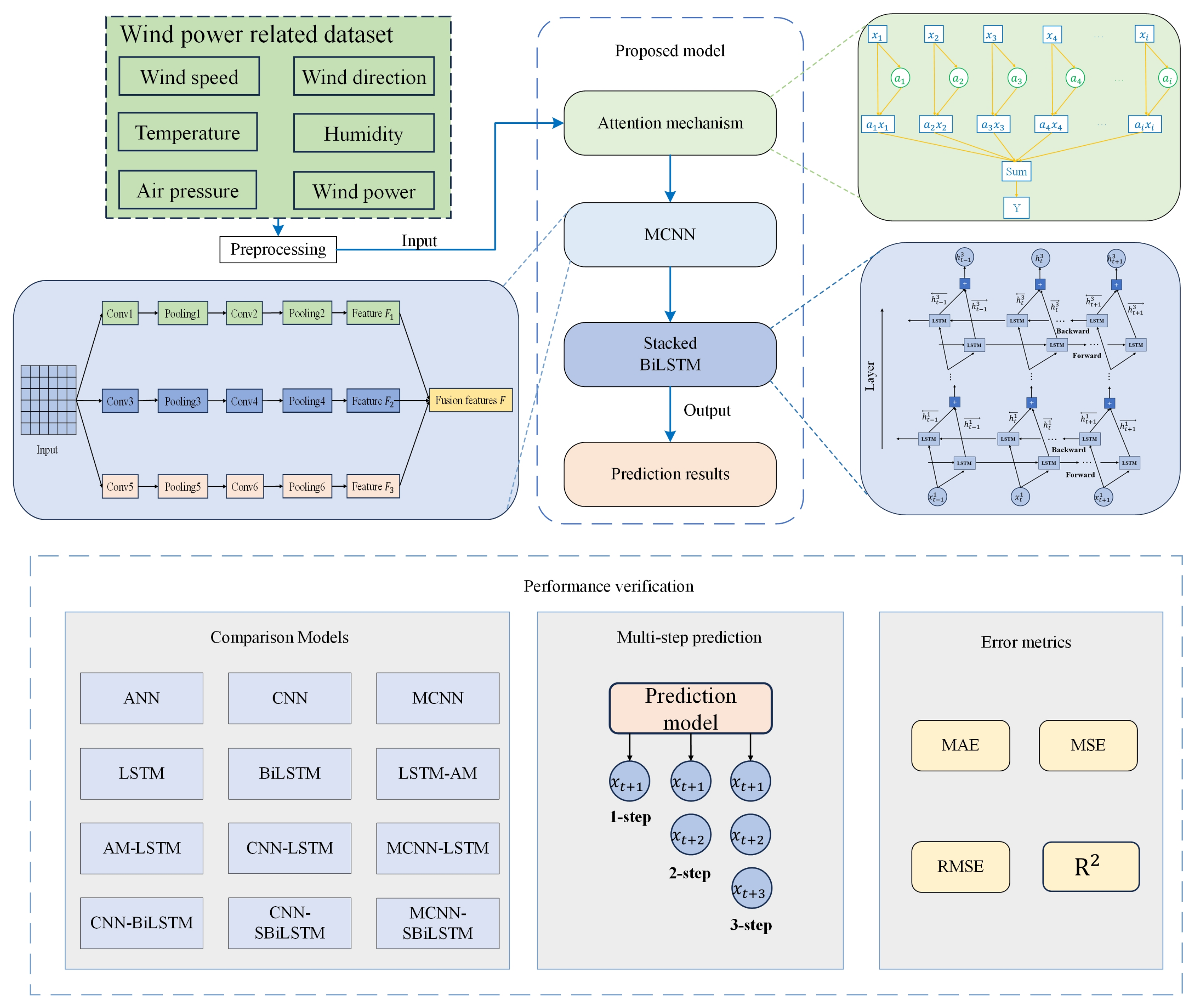
In summary, distinguishing the importance of different wind power characteristics and exploring a combination model that can fully extract input feature information and capture the time dependency of feature sequences is a major challenge to improve prediction accuracy. Therefore, this paper proposes a wind power prediction method based on feature weighting and combination models to overcome the limitations of existing methods and achieve higher accuracy predictions. This article makes the following contributions:

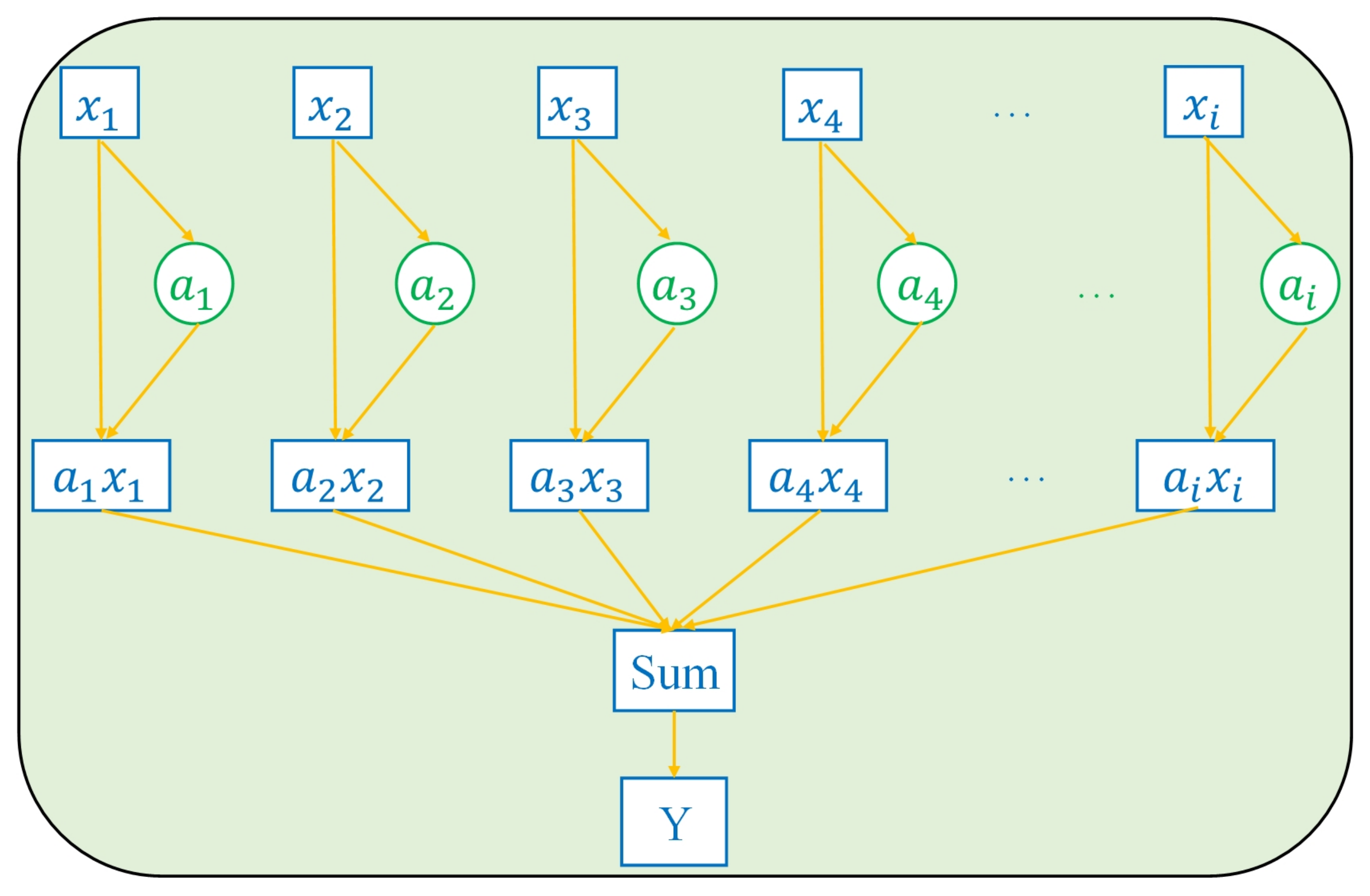
• The attention mechanism is used to dynamically assign the weights of each input feature to distinguish the importance of different features on the impact of wind power output. In addition, the order in which the attention mechanism is introduced allows the model to be more focused on the information that is more important to the prediction results when extracting features.
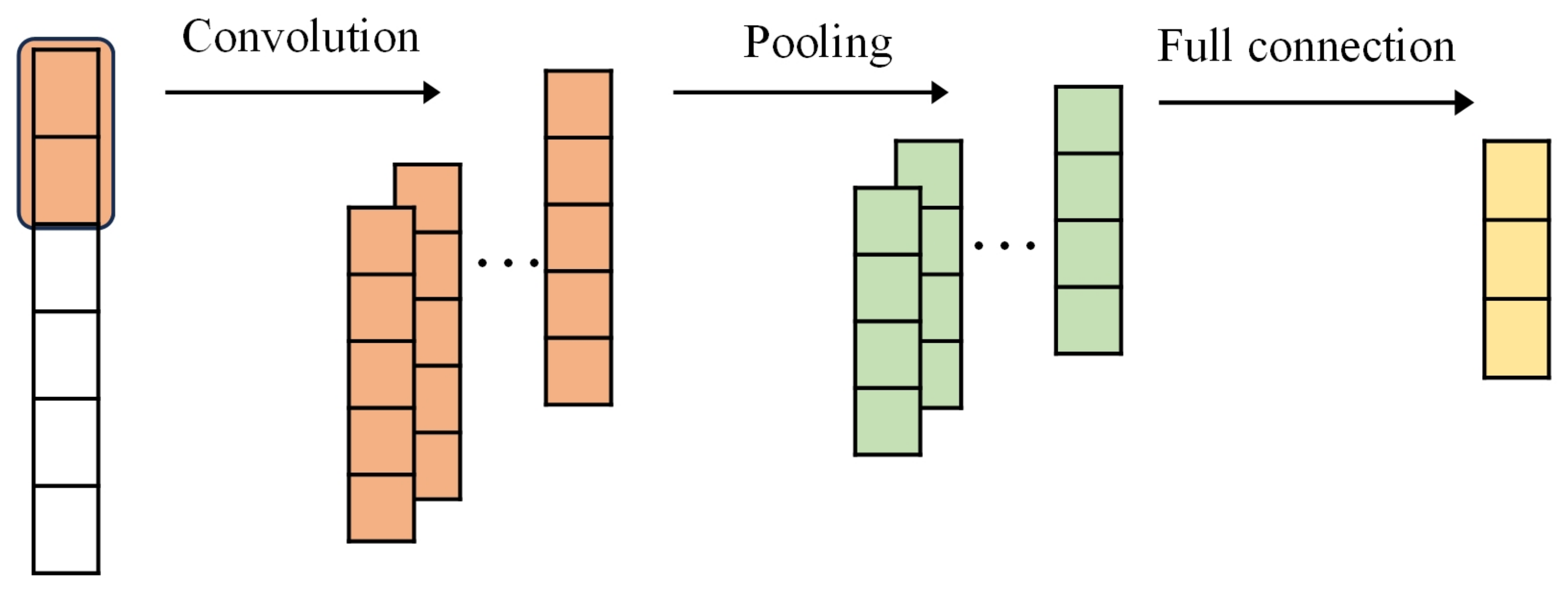
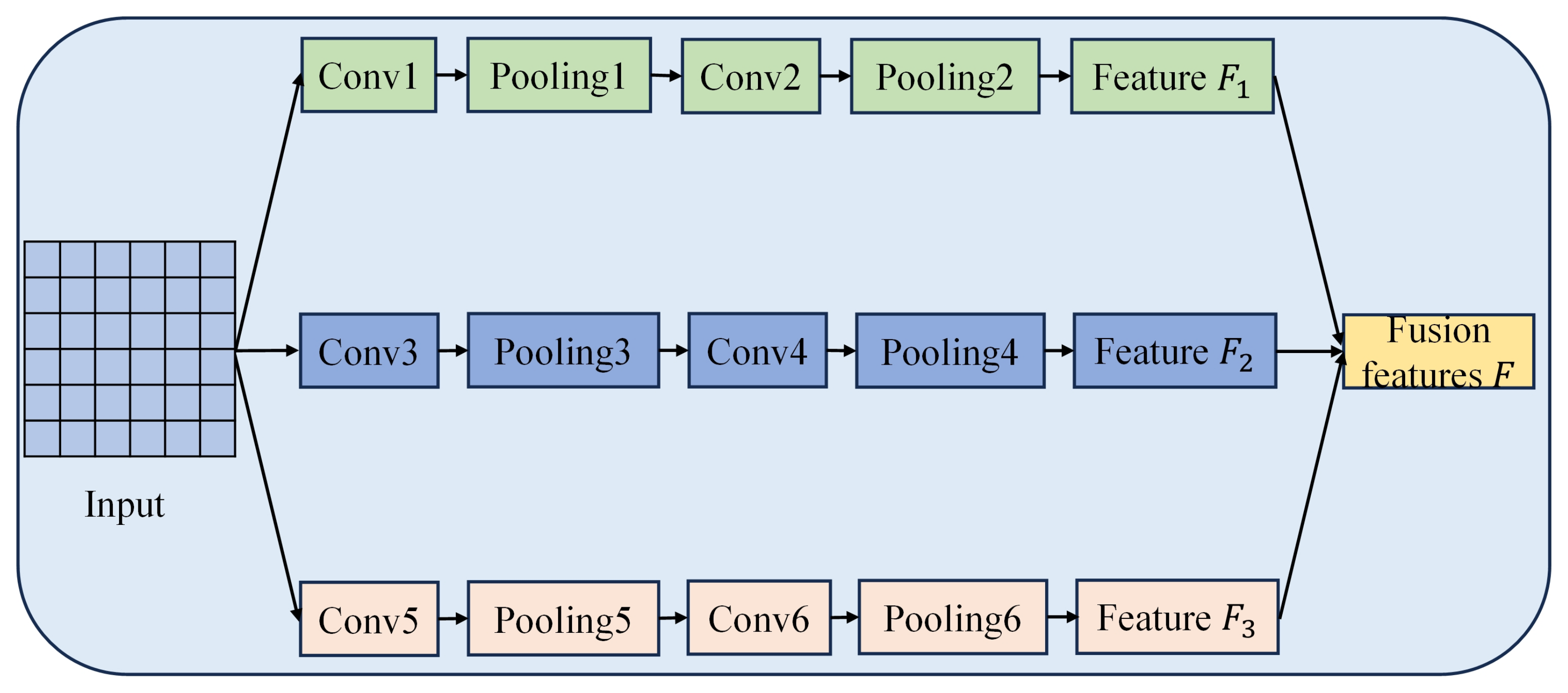
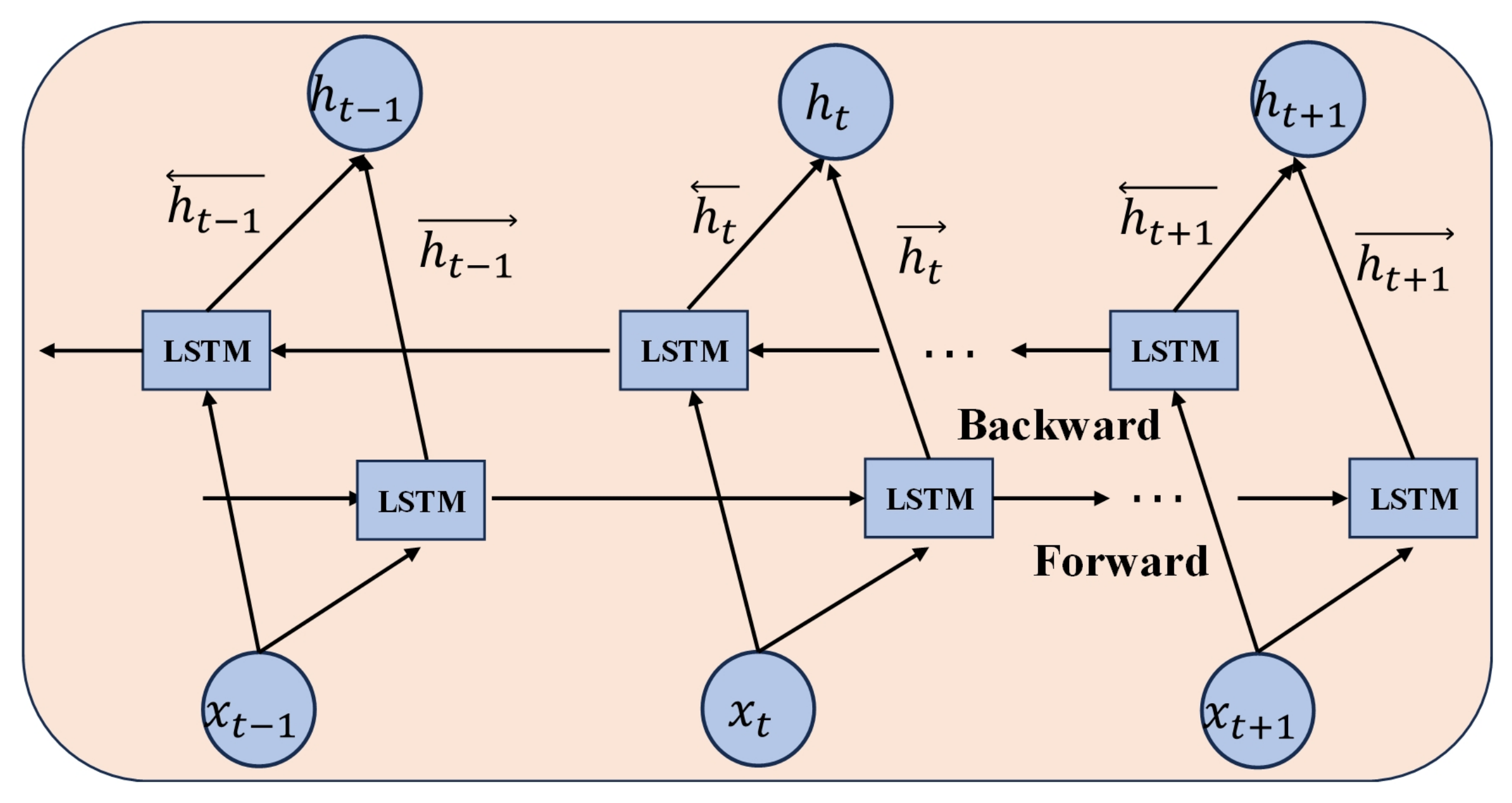
• The MCNN with different convolutional kernels can extract the feature information of different scales more comprehensively. SBiLSTM can better capture the temporal dependencies of feature sequences. The two neural networks in the combined model play to their respective strengths, enhancing the model’s capacity to extract features and their long-term trends.
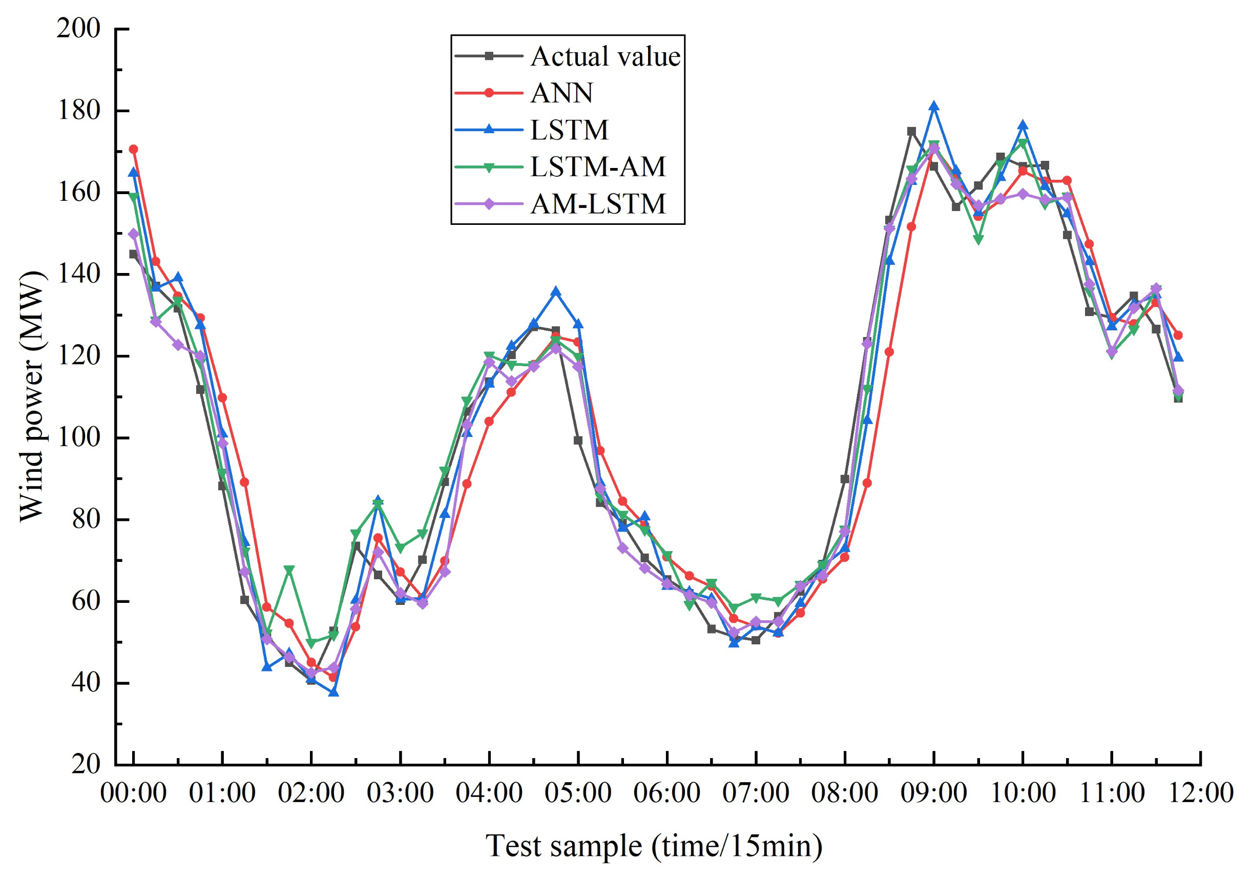
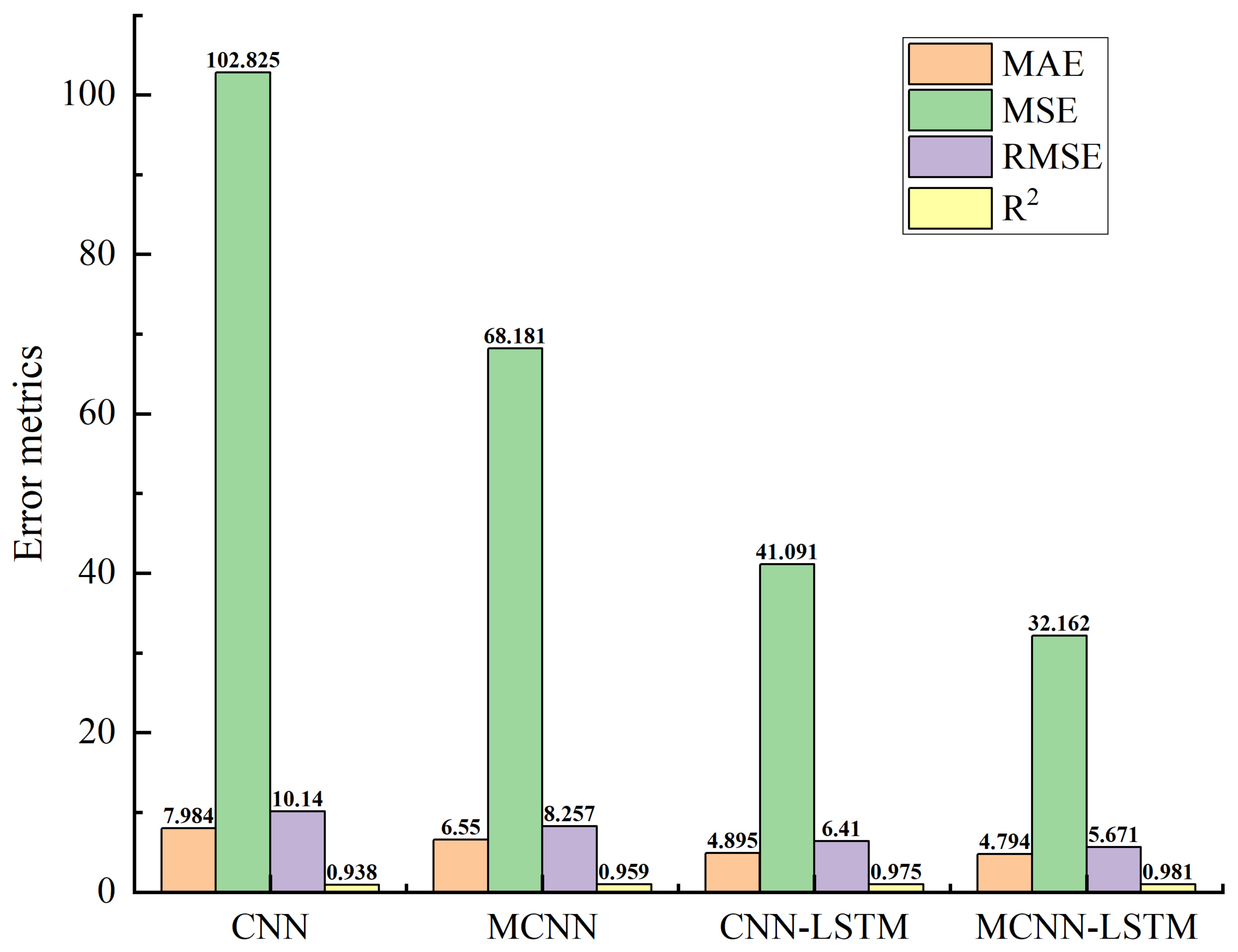
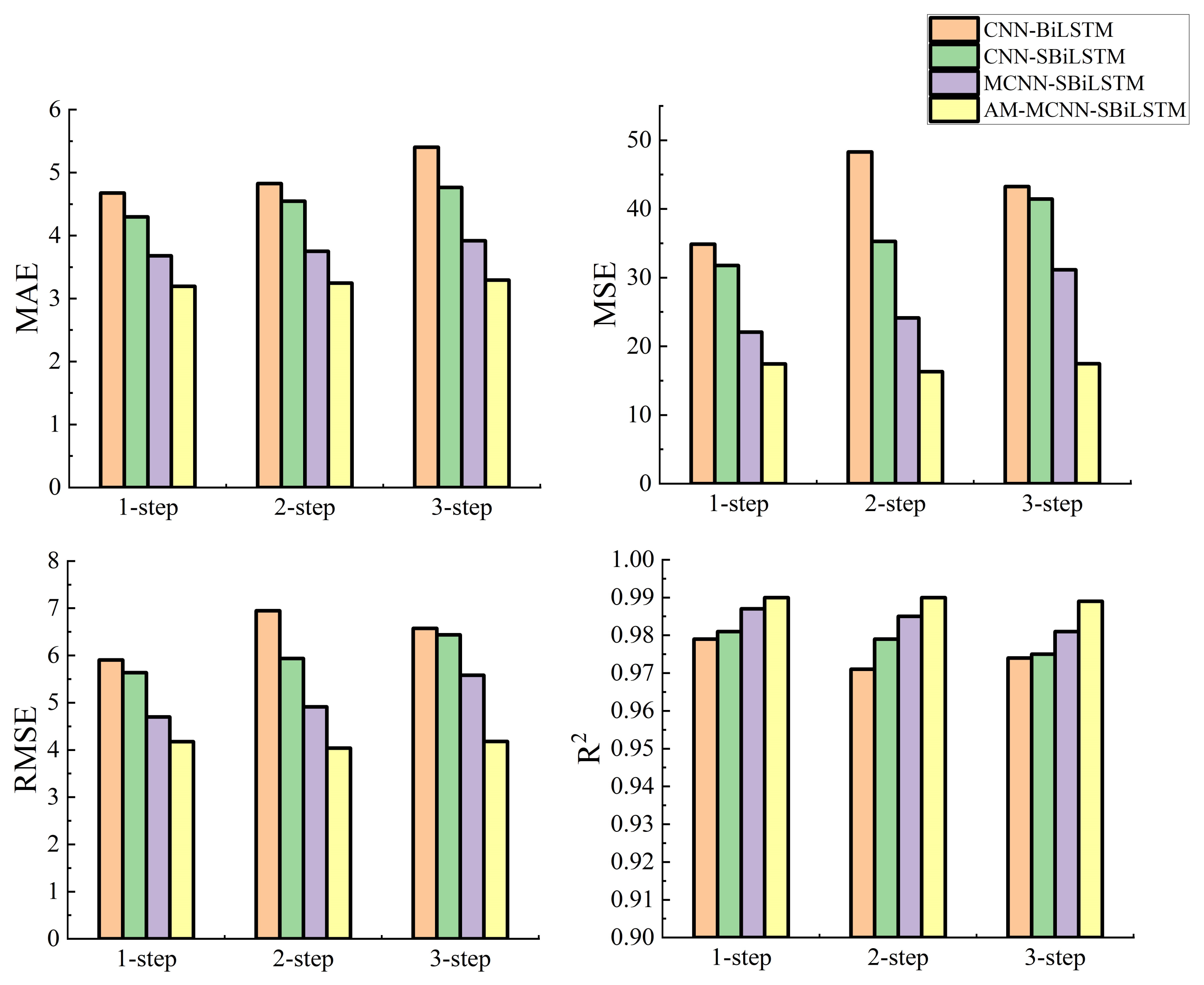
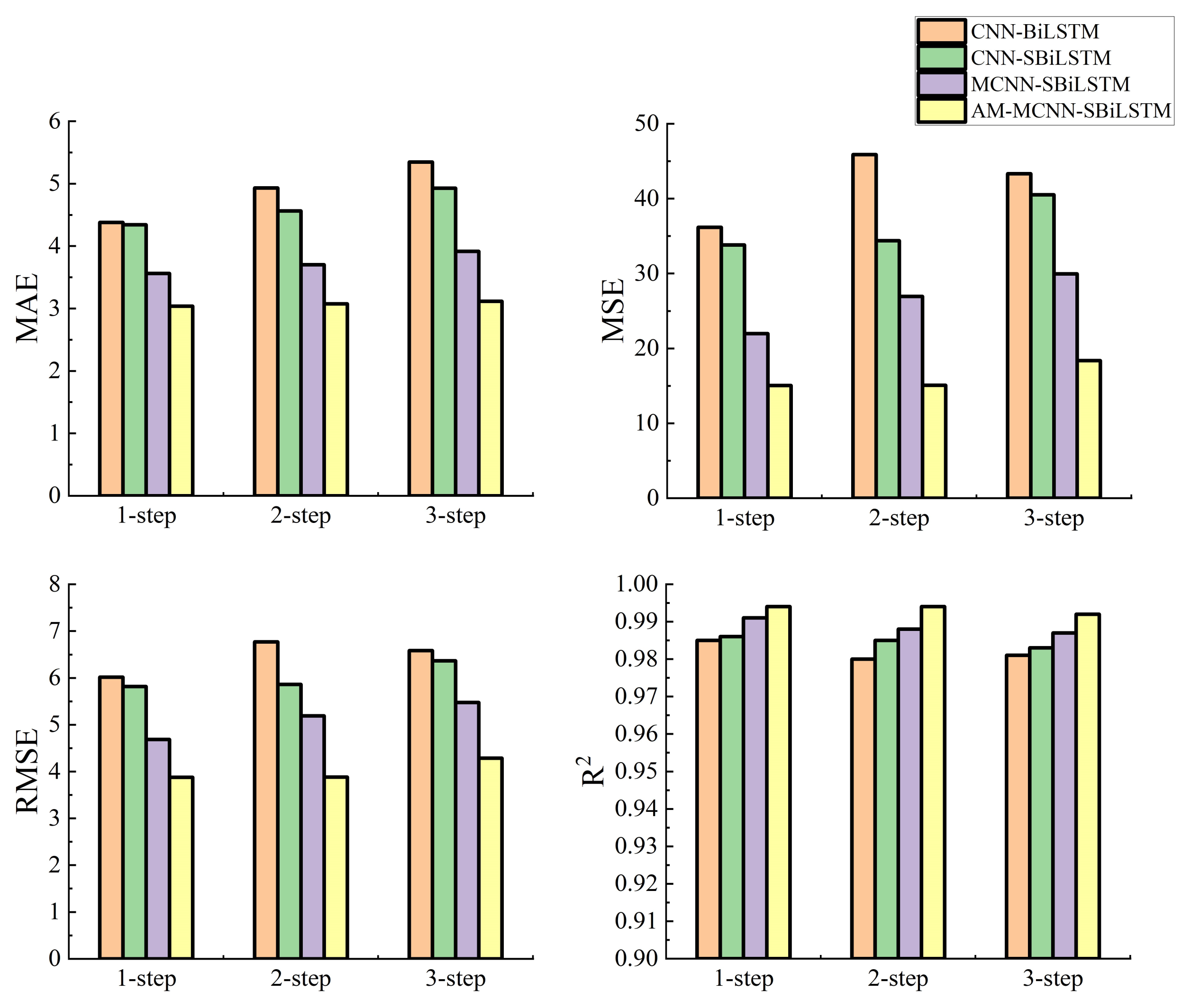
• Using real wind farm data, four groups of comparative experiments are carried out to verify the effectiveness and stability of the proposed method; based on four commonly used error indicators, the proposed models all demonstrated the best prediction accuracy.

The remainder of this article is structured as follows: Section 2 includes the materials and methods; it first introduces the wind power-related datasets, then describes the prediction process of the proposed model, focusing on the individual modules in the ensemble model. Finally, the overall prediction framework of the method when applied to actual cases is introduced. Section 3 conducts experiments and analyzes the results. Section 4 draws conclusions.

2. Materials and Methods

2.1. Wind Power-Related Dataset

The wind power-related dataset is defined as sequence $X={\left[\begin{array}{c}{X}_1,X_2,\dots ,X_t\end{array}\right]}^T$, where $X_t$ represents sequential data at different time points, which can be represented as $X_t$ $=\left[\begin{array}{c}{x}_1,x_2,\dots ,x_i\end{array}\right]$, where $x_i$ represents various meteorological factors related to wind power. The dataset used in this article comes from the actual operation data of the Hami Wind Farm in Xinjiang, China. It includes wind speed and wind direction information at 10 m, 30 m, and 50 m on the measurement tower, as well as meteorological information such as temperature, humidity, pressure, and historical wind power. The data were collected between 1 January 2022 and 30 January 2022, resulting in a total of 2880 data observations. The sampling frequency was 15 min.

2.2. Proposed Model

2.2.1. AM-MCNN-SBiLSTM

Figure 1 depicts the prediction process of the AM-MCNN-SBiLSTM model. The wind-related dataset is input into the attention mechanism for feature weighting, obtaining the weighted feature sequence. The weighted feature data is then input into the Multi-Convolutional Neural Network (MCNN) for feature extraction. The extracted multi-scale fusion feature information serves as the input for the Stacked BiLSTM (SBiLSTM) networks, capturing the temporal dependencies of the fusion feature sequence. The final forecast value is obtained through a fully connected layer.

Figure 1. Prediction flow of the proposed model.

The attention mechanism distinguishes the contribution of different features to the output by learning the associated information in sequence data, facilitating the model’s better capturing of critical information. The MCNN employs a parallel processing of convolutional kernels of varying sizes, enabling a more comprehensive and efficient extraction of features across different time scales, thereby enhancing the model’s capacity to express features. BiLSTM can capture the long-term trends in feature sequences. By stacking BiLSTM layers, the model’s depth is increased, allowing it to learn more complex data patterns and relationships.

2.2.2. Attention Mechanism

The attention mechanism is an extensively employed technology in machine learning, which essentially involves the weighted summation of sequences. By adaptively assigning different weights to input variables, it distinguishes the importance of different variables on the output [35]. In this work, we utilize an attention mechanism to dynamically allocate varying weights to different input features, assigning higher weights to important features and lower weights to unimportant ones [36], highlighting the important parts of input features that affect wind power output. The input features are reconstructed into a new feature sequence based on the assigned weights. Its working principle is shown in Figure 2.

Figure 2. Attention mechanism.

The formula for allocating weights in the attention mechanism is as follows:

$$e_i=utanh\left({\omega }_1{x}_i+b_1\right)$$

(1)

$$a_i={\displaystyle \frac{exp\left(e_i\right)}{{\sum }_{i=1}^{i}exp\left(e_i\right)}}$$

(2)

$$Y=\sum _{i=1}^i{a}_i{x}_i$$

(3)

$x_i$ represents i-th input feature data, $e_i$ represents the attention probability distribution values corresponding to $x_i$. $\mathit{u}$ and ${\omega }_1$ are weights, $b_1$ represents bias. $a_i$ is obtained by the exponential non-linear transformation of $e_i$, aiming to make the attention probability distribution more flexible to adapt to different input data. $a_i$ can be seen as the weight of each feature; the larger $a_i$ is, the more contribution the input feature makes to the output. $\mathit{Y}$ is the weighted new feature sequence.

2.2.3. Multi-Convolutional Neural Networks (MCNNs)

The CNN has achieved great success in image recognition due to its powerful feature extraction capability [37]. The reason for its success lies in the use of local connections and weight sharing, which reduces the number of weights and makes the network easier to optimize [38]. The CNN is mainly composed of convolutional layers, pooling layers, and fully connected layers. Using one-dimensional convolution to handle time series problems can not only maintain the continuity of sequence information but also improve computational efficiency [39]. Figure 3 shows the basic structure of a 1-D CNN.

Figure 3. 1-D CNN.

In wind power sequence data, there are features at multiple time scales. By using multi-convolutions with various kernels, feature information can be more comprehensively extracted. This paper selects the MCNN with three convolution kernels (2, 3, 5) for feature extraction, constructing independent 1-D convolutions for each kernel. The input data undergo convolution operations simultaneously with three different kernels. For the output of each kernel, max-pooling is applied on the feature maps to further reduce the feature dimension and retain the most significant features. By performing two convolution operations for each kernel, the three parallel convolution layers of different scales fully extract features. These features are fused together to form a higher-dimensional feature representation. The MCNN is shown in Figure 4.

Figure 4. The structure of the MCNN.

Formula (4) represents the convolution operation:

$$y_i=f({\omega }_2\otimes X+b_2)$$

(4)

$y_{\mathrm{i}}$ is the output after applying the i-th convolutional kernel. $\mathit{f}$ is the activation function that introduces non-linear feature transformations to the input, with ReLU being the activation function. ⊗ represents the convolution operation, $\mathit{X}$ is the data tensor, ${\omega }_2$ is the weight of the convolutional kernel, and $b_2$ is the bias needed in the network learning process.

$$\widehat{y_i}=poo{l}_{\max }\left(y_i\right)$$

(5)

$$F_i=poo{l}_{\max }\left(conv\left(\widehat{y_i}\right)\right)$$

(6)

$$F=Concat(F_1,F_2,F_3)$$

(7)

The output after convolution is processed by the Formula (5) for the max pooling layer, with $\widehat{y_i}$ representing the pooled feature sequence. Formula (6) performs convolution and pooling operations again, and each convolution kernel finally extracts the feature $F_i$. The features successfully extracted by three types of convolutional kernels are $F_1$, $F_2$, and $F_3$, and the fused new feature $\mathit{F}$ is shown in Formula (7). The fused new feature prepares for extracting the time-dependent trend of the feature sequence in the next step.

2.2.4. Stacked BiLSTM (SBiLSTM) Networks

Past and future information within the wind power sequence can influence prediction outcomes [40]. In comparison to the unidirectional propagation utilized by LSTM, BiLSTM concatenates sequence features and corresponding hidden states through forward and backward propagation, enabling bidirectional feature extraction [41]. In this way, BiLSTM can more comprehensively capture and understand the contextual information of wind-related sequences, including past and future trends. Figure 5 describes the architecture of the BiLSTM.

Figure 5. The structure of the BiLSTM.

The formula for updating bidirectional state information in the BiLSTM is as follows [42]:

$$\overrightarrow{h_t}=\overline{LSTM}(x_t,\overrightarrow{h_{t-1}})$$

(8)

$$\overleftarrow{h_t}=\overline{LSTM}(x_t,\overleftarrow{h_{t+1}})$$

(9)

$$h_t={\omega }_3\overrightarrow{h_t}+{\omega }_4\overleftarrow{h_t}+c_t$$

(10)

Among them, $\overline{LSTM}$ is the LSTM calculation process. At time t, $x_t$ represents the input, while $\overrightarrow{h_t}$ and $\overleftarrow{h_t}$ represent the bidirectional sequence information. $\overrightarrow{h_{t-1}}$ and $\overleftarrow{h_{t+1}}$ denote the forward and backward sequence information of the preceding instant. $y_t$ is the output information, ${\omega }_3$ and ${\omega }_4$ are the forward and backward weights, respectively, while $c_t$ stands for the bias parameter.

The number of layers in BiLSTM is an important hyperparameter that governs model learning. In this paper, we first assume that stacked three-layer BiLSTM is used to obtain richer and more complex temporal information, and we will subsequently employ specific experiments to verify the correctness of this assumption. The bottom BiLSTM layer can capture the basic temporal relationships of the sequence, and as the layers increase, the model can gradually learn more abstract and higher-level hidden information. The stacked BiLSTM layers are shown in Figure 6.

Figure 6. Stacked BiLSTM.

The output from the preceding layer shall serve as input for the succeeding one. The final output of each layer is obtained by merging the forward and backward hidden states. The updating of the state information for each layer is as follows [43]:

$$h_t^1=[\overrightarrow{h_t^1};\overleftarrow{h_t^1}]$$

(11)

$$h_t^2=[\overrightarrow{h_t^2};\overleftarrow{h_t^2}]$$

(12)

$$h_t^3=[\overrightarrow{h_t^3};\overleftarrow{h_t^3}]$$

(13)

The first layer BiLSTM network takes $x_t^1$ as input and output $h_t^1$, $\overrightarrow{h_t^1}$ and $\overleftarrow{h_t^1}$, representing the hidden state information of the bidirectionalityof the first layer at time step t. The second BiLSTM layer receives input $h_t^1$ and generates output $h_t^2$. The third layer has an input of $h_t^2$ and an output of $h_t^3$. $h_t^3$ is connected with the fully connected layer to obtain the final result, as shown in Equation (14).

$$z=W_{fc}·h_t^3+b_{fc}$$

(14)

The weight matrix is represented by $W_{fc}$, $b_{fc}$ is the bias term, and $\mathit{z}$ is the result of weighted sum. To mitigate the issue of model degradation caused by the deepening of networks, we incorporate dropout technology into the BiLSTM layer.

2.3. Overall Prediction Framework for the Proposed Method: A Real Case

As illustrated in Figure 7, the proposed method is applied to the overall predictive framework for a real-case scenario. It mainly includes the preprocessing of the original data, prediction using the AM-MCNN-SBiLSTM model, and performance verification. The specific process is described as follows:

Figure 7. Overall framework for the application of the proposed model to a real case.

(1) The wind power-related dataset includes meteorological characteristics such as wind speed, wind direction, temperature, humidity, air pressure, and historical wind power. In the subsequent experiments, the model’s predictive performance was assessed by dividing the dataset into a training set comprising the first $95\%$, and a test set consisting of the remaining $5\%$ [44,45].

(2) Typically, the information collected from wind farms inevitably embodies disparities in numeric dimensions across various characteristics. In order to transform the raw data into an input that the model can understand, we performed data min–max normalization on the collected dataset. It employs a common normalization method that maps data linearly onto the range of [0,1], as depicted by Equation (15).

$$x_{nomn}={\displaystyle \frac{x-x_{min}}{x_{max}-x_{min}}}$$

(15)

$x_{norm}$ is the normalized value, $\mathit{x}$ is the original value in the dataset, and $x_{max}$ and $x_{min}$ are the maximum and minimum values in the dataset.

(3) Input the preprocessed dataset into the attention mechanism to obtain a weighted new feature sequence. The new feature sequence is used as the input for the MCNN to fuse the high-dimensional features extracted by different convolutional kernels. The fused feature information is then input into a stacked three-layer BiLSTM network to obtain the prediction result. To give the data physical meaning, perform inverse normalization on the predicted results using the following formula:

$$x_{dnorm}^{*}=(x_{max}-x_{min})x^{*}+x_{min}$$

(16)

In the formula, $x_{dnorm}^{*}$ represents the final prediction value, and $x^{*}$ represents the normalized prediction value.

(4) To verify the efficacy of proposed methodologies from multiple perspectives, we selected an ANN, LSTM, LSTM-AM, and AM-LSTM as the first group of comparative models to study the impact of introducing the attention mechanism on prediction results in the model. The CNN, MCNN, CNN-LSTM, and MCNN-LSTM were chosen as the second group of comparative models to verify the advantages of multi-convolutional neural networks in prediction. Different layers of BiLSTM networks were selected for the third group of comparative experiments to explore the influence of BiLSTM layers on prediction results. CNN-BiLSTM, CNN-SBiLSTM, and MCNN-SBiLSTM models were chosen for the fourth group of comparative experiments along with the proposed AM-MCNN-SBiLSTM prediction model to further validate the effectiveness of the proposed model. All the hybrid models mentioned above are composed of single models, and the specific descriptions of each single model can be found in Table 1. The batch size is set to 64, with the previous time step set to 96, the number of iteration epochs is 120, and the Adam optimizer is selected. All models were trained several times, and finally, the best parameters that do not produce overfitting were selected, as shown in Table 2.

Table 1. Nomenclature.

Abbreviation	Specific Description
NWP	Numerical weather prediction
ARMA	Autoregressive moving average
ARIMA	Autoregressive integrated moving average
ANN	Artificial neural network
SVM	Support vector machine
RNN	Recurrent neural network
LSTM	Long short-term memory
GRU	Gated recurrent unit
CNN	Convolutional neural network
BiLSTM	Bidirectional Long Short-Term Memory
KDE	Kernel density estimation
VMD	Variational mode decomposition
WPE	Weighted permutation entropy
MCNN	Multi-convolutional neural networks
SBiLSTM	Stacked bidirectional long short-term memory
AM	Attention mechanism
MAE	Mean absolute error
MSE	Mean squared error
RMSE	Root mean squared error
${\mathrm{R}}^2$	Coefficient of determination

Table 2. All model network parameters’ selection.

Model	Specific Description
ANN	layer = 1; hidden neurons = 16
CNN	filters = 32; kernel size = 2; pooling kernel = 2; stride = 1
LSTM	layer = 1; hidden neurons = 128
BiLSTM	layer = 1; hidden neurons = 128
MCNN	Conv1	filters = 32; kernel size = 2; stride = 1
	Pooling1	kernel size = 2; stride = 1
	Conv2	filters = 64; kernel size = 2; stride = 1
	Pooling2	kernel size = 2; stride = 1
	Conv3	filters = 32; kernel size = 3; stride = 1
	Pooling3	kernel size = 2; stride = 1
	Conv4	filters = 64; kernel size = 3; stride = 1
	Pooling4	kernel size = 2; stride = 1
	Conv5	filters = 32; kernel size = 5; stride = 1
	Pooling5	kernel size = 2; stride = 1
	Conv6	filters = 64; kernel size = 5; stride = 1
	Pooling6	kernel size = 2; stride = 1
SBiLSTM	layers = 3; hidden neurons = 128
dropout	0.01

(5) By changing the prediction step size for multi-step prediction to verify the stability of the prediction model, four common error metrics are used to evaluate the performance of each model, including MAE, MSE, RMSE, and $R^2$, as shown in Formulas (17) to (20).

$$MAE={\displaystyle \frac{1}{N}}\sum _{i=1}^N|{\widehat{p}}_i-p_i|$$

(17)

$$MSE={\displaystyle \frac{1}{N}}\sum _{i=1}^N{({\widehat{p}}_i-p_i)}^2$$

(18)

$$RMSE=\sqrt{{\displaystyle \frac{1}{N}}\sum _{i=1}^N{\left({\widehat{p}}_i-p_i\right)}^2}$$

(19)

$$R^2=1-{\displaystyle \frac{{\sum }_{i=1}^N{\left({\widehat{p}}_i-p_i\right)}^2}{{\sum }_{i=1}^N{\left(\overline{p}-p_i\right)}^2}}$$

(20)

$p_i$ and $\widehat{p_i}$ are the actual and predicted values of wind power at time i, $\overline{p}$ is the average value, and N is the total number of predicted values. The smaller the error indicators of MAE, MSE, and RMSE are, the better the performance of the model is, while $R^2$ value is the opposite.

3. Results and Discussion

3.1. Experimental Platform

The experimental platform in this article is a personal computer with a 12th Gen Intel(R) Core(TM) i9-12900KF processor (Intel, Santa Clara, CA, USA) and an NVIDIA (NVIDIA, Santa Clara, CA, USA) GeForce RTX 3080 Ti GPU. All experiments were implemented based on the open-source deep learning framework PyCharm (version 2022.1.3) and Cuda (version 11.6).

3.2. Prediction and Analysis

3.2.1. Experiment I: The Impact of the Attention Mechanism

It is obvious from Figure 8 that without adding an attention mechanism to the model, the model’s predicted values fluctuate significantly compared to the true values. Additionally, the order of introducing attention mechanisms also leads to differences in prediction performance.

Figure 8. Prediction curves of different models.

Table 3 shows that the LSTM exhibits a significantly lower prediction error compared to the ANN, indicating that the LSTM has better non-linear fitting capability when dealing with wind power sequence data. The MAE, MSE, RMSE, and ${\mathrm{R}}^2$ values of LSTM-AM are 7.072, 76.694, 8.758, and 0.954, respectively, which are $10.38\%$, $24.93\%$, $13.35\%$, $1.71\%$ higher than the error values of LSTM. This indicates that the prediction accuracy can be improved by adding the attention mechanism to the model. The four error metric values of AM-LSTM are 6.260, 60.582, 7.784, and 0.963, which are $11.48\%$, $21.01\%$, $11.12\%$, and $0.94\%$ higher than the error performance of LSTM-A. This suggests that using the attention mechanism before the LSTM model can better leverage its advantages compared to using the attention mechanism after LSTM. Through analysis, this order can assist the model in more effectively utilizing the information of the input data, reduce information loss, and learn feature representations more flexibly.

Table 3. Error metrics for prediction models (The best value of the data has been bolded, the following tables are the same).

Model	MAE	MSE	RMSE	R2
ANN	11.282	196.680	14.024	0.881
LSTM	7.891	102.159	10.107	0.938
LSTM-AM	7.072	76.694	8.758	0.954
AM-LSTM	6.260	60.582	7.784	0.963

3.2.2. Experiment II: The Impact of Multiple Convolutions

As observed from Table 4 and Figure 9, it is apparent that CNN-LSTM and MCNN-LSTM exhibit lesser prediction errors compared to the CNN and the MCNN, indicating that the combination models can utilize the advantages of multiple models to improve predictive accuracy. Specifically, the MAE, MSE, RMSE, and $R^2$ values of the MCNN are 6.550, 68.181, 8.257, and 0.959, respectively, which are $17.96\%$, $33.69\%$, $18.57\%$, and $2.24\%$ higher than those of the CNN. Similarly, compared to CNN-LSTM, the four error metrics of MCNN-LSTM have increased by $2.06\%$, $21.73\%$, $11.53\%$, and $0.62\%$. The above data indicate that using the MCNN with multiple parallel convolutional kernels can more comprehensively extract features of different scales and more accurately predict future wind power values.

Table 4. Error metrics for prediction models.

Model	MAE	MSE	RMSE	R2
CNN	7.984	102.825	10.140	0.938
MCNN	6.550	68.181	8.257	0.959
CNN-LSTM	4.895	41.091	6.410	0.975
MCNN-LSTM	4.794	32.162	5.671	0.981

Figure 9. Comparison of predictive performances of various models.

3.2.3. Experiment III: The Impact of BiLSTM Layers

As shown in Figure 10, it is evident that the prediction curve is most closely aligned with the actual value curve when the number of stacking layers is three. Analyzing the data in Table 5, it can be found that when stacking three layers of BiLSTM, all error metrics are optimal. Compared to a single layer of BiLSTM, the MAE, MSE, RMSE, and $R^2$ values of the three-layer BiLSTM increased by $17.95\%$, $32.19\%$, $17.65\%$, and $1.35\%$, respectively. Similarly, compared to the two-layer BiLSTM, the four error metrics increased by $5.97\%$, $2.42\%$, $1.21\%$, and $0.10\%$, respectively. This indicates that stacking three layers of a BiLSTM network can learn more advanced and richer feature representations, better capture the temporal relationships between data, and improve prediction accuracy. However, when the number of layers is four, the prediction accuracy decreases. Through analysis, it is found that too many stacked layers will increase the complexity of the model, reduce its interpretability, and thus affect the prediction performance.

Figure 10. Prediction curves of BILSTM for different layers.

Table 5. Error metrics for BiLSTM with different numbers of layers.

Model	MAE	MSE	RMSE	R2
One layer	6.255	64.357	8.022	0.961
Two layers	5.458	44.718	6.687	0.973
Three layers	5.132	43.638	6.606	0.974
Four layers	6.542	66.495	8.155	0.960

3.2.4. Experiment IV: The Performance of the Proposed Model

As depicted in Figure 11, the predicted curve of the proposed model in the test samples closely aligns with the trend of the true values curve, and in Table 6, the AM-MCNN-SBiLSTM has the highest prediction accuracy, which all indicates that the model possesses remarkable predictive capabilities. In wind power forecasting, multi-step prediction is achieved by changing the future time steps to be predicted. In Table 7, the AM-MCNN-SBiLSTM model still has the highest prediction accuracy in two-step and three-step predictions. It can be further concluded from the comparison between the AM-MCNN-SBiLSTM and MCNN-SBiLSTM models that weighting the input feature data with attention can help improve the prediction accuracy. The predictions made by MCNN-SBiLSTM consistently outperformed those of CNN-SBiLSTM, which further validates the stronger feature extraction capability of multiple convolutions. Similarly, CNN-SBiLSTM outperforms CNN-BiLSTM in all four error metrics, once again proving that stacking three layers of BiLSTM has a more comprehensive learning ability for wind power data.

Figure 11. The predicted curve of the proposed model.

Table 6. Error metrics for 1-step forecasts: 12 h ahead of schedule.

Model	MAE	MSE	RMSE	R2
CNN-BiLSTM	4.676	34.857	5.904	0.979
CNN-SBiLSTM	4.299	31.764	5.636	0.981
MCNN-SBiLSTM	3.681	22.081	4.699	0.987
AM-MCNN-SBiLSTM	3.194	17.424	4.174	0.990

Table 7. Error metrics for 2-step, 3-step forecasts: 12 h ahead of schedule.

Model	2-Step				3-Step
	MAE	MSE	RMSE	R2	MAE	MSE	RMSE	R2
CNN-BiLSTM	4.827	48.281	6.949	0.971	5.405	43.245	6.576	0.974
CNN-SBiLSTM	4.548	35.270	5.939	0.979	4.764	41.431	6.437	0.975
MCNN-SBiLSTM	3.752	24.124	4.912	0.985	3.920	31.157	5.582	0.981
AM-MCNN-SBiLSTM	3.245	16.297	4.037	0.990	3.292	17.465	4.179	0.989

Figure 12 demonstrates that the prediction performance of the contrast models fluctuates significantly as the prediction horizon increases. In contrast, the AM-MCNN-SBiLSTM model shows only slight variations in its error metrics. This indicates that the proposed model exhibits more efficient and stable predictive performance compared to other models, and can better describe the changing trends of wind power sequences.

Figure 12. Comparison of multi-step, 12 h ahead forecasting performance.

To further validate the model’s performance, the time resolution range is adjusted from 12 h ahead to 24 h ahead. In Table 8 and Table 9, the error metrics of the proposed AM-MCNN-SBiLSTM model are still optimal under different step sizes. The $R^2$ values for one-step, two-step, and three-step forecasts are 0.994, 0.994, and 0.992 respectively. Figure 13 depicts the $R^2$ fit effectiveness of the proposed model for multi-step predictions, indicating a high degree of compatibility between predicted values and actual observed data, as well as greater reliability in prediction performance.

Table 8. Error metrics for 1-step forecasts: 24 h ahead of schedule.

Model	MAE	MSE	RMSE	R2
CNN-BiLSTM	4.380	36.180	6.015	0.985
CNN-SBiLSTM	4.341	33.823	5.816	0.986
MCNN-SBiLSTM	3.562	21.964	4.687	0.991
AM-MCNN-SBiLSTM	3.038	15.048	3.879	0.994

Table 9. Error metrics for 2-step, 3-step forecasts: 24 h ahead of schedule.

Model	2-Step				3-Step
	MAE	MSE	RMSE	R2	MAE	MSE	RMSE	R2
CNN-BiLSTM	4.932	45.864	6.772	0.980	5.346	43.327	6.582	0.981
CNN-SBiLSTM	4.565	34.383	5.864	0.985	4.928	40.505	6.364	0.983
MCNN-SBiLSTM	3.702	26.934	5.190	0.988	3.916	29.964	5.474	0.987
AM-MCNN-SBiLSTM	3.076	15.069	3.882	0.994	3.115	18.375	4.287	0.992

Figure 13. $R^2$ prediction fitting effect of 1-step, 2-step, and 3-step performance.

As the forecast horizon increases in Figure 14, our proposed model still shows more stable forecasting performance compared to other models. These all indicate that AM-MCNN-SBiLSTM possesses not only excellent forecasting capabilities but also exhibits good robustness when facing longer forecasting time spans.

Figure 14. Comparison of multi-step ahead 24 h forecasting performance.

4. Conclusions

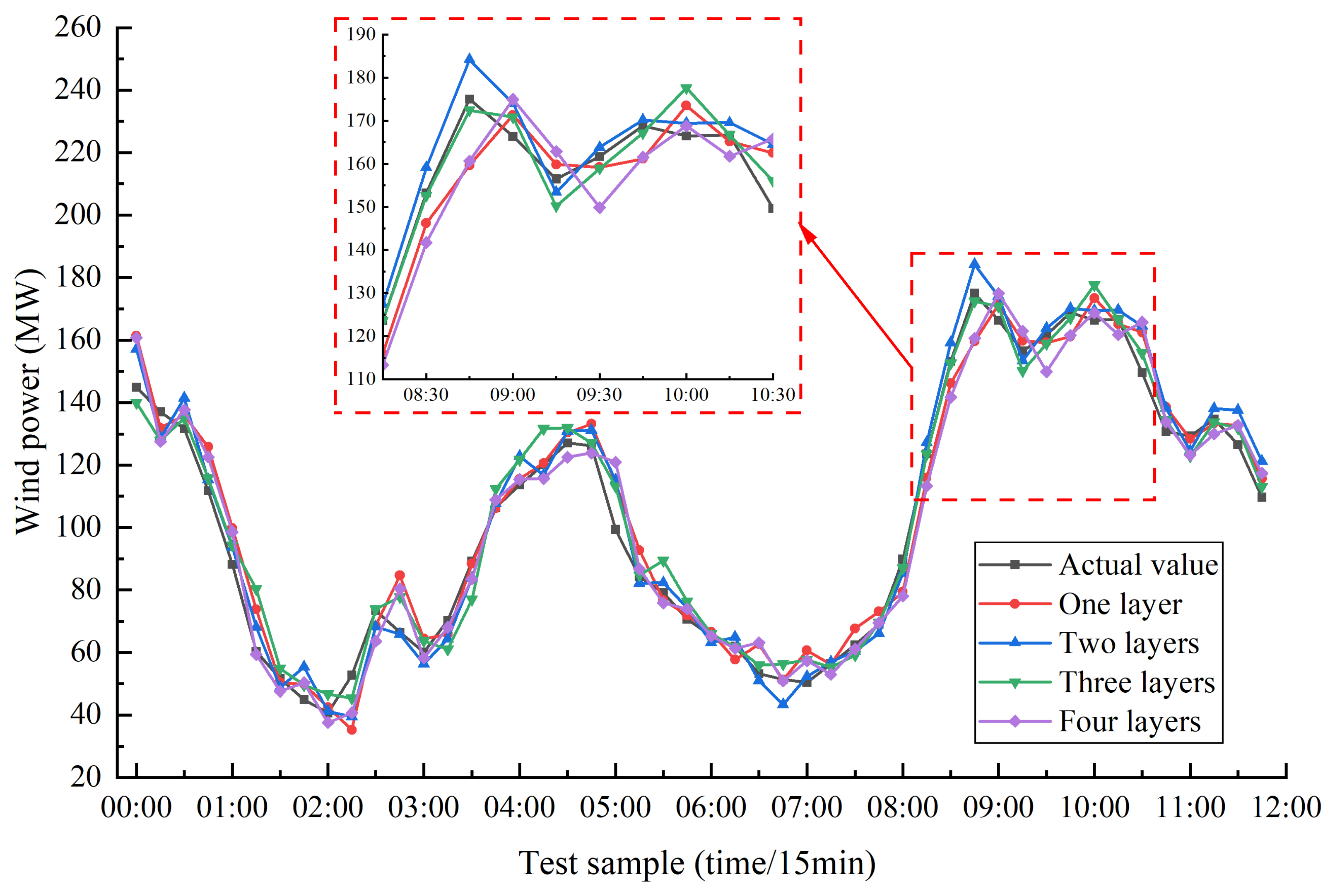
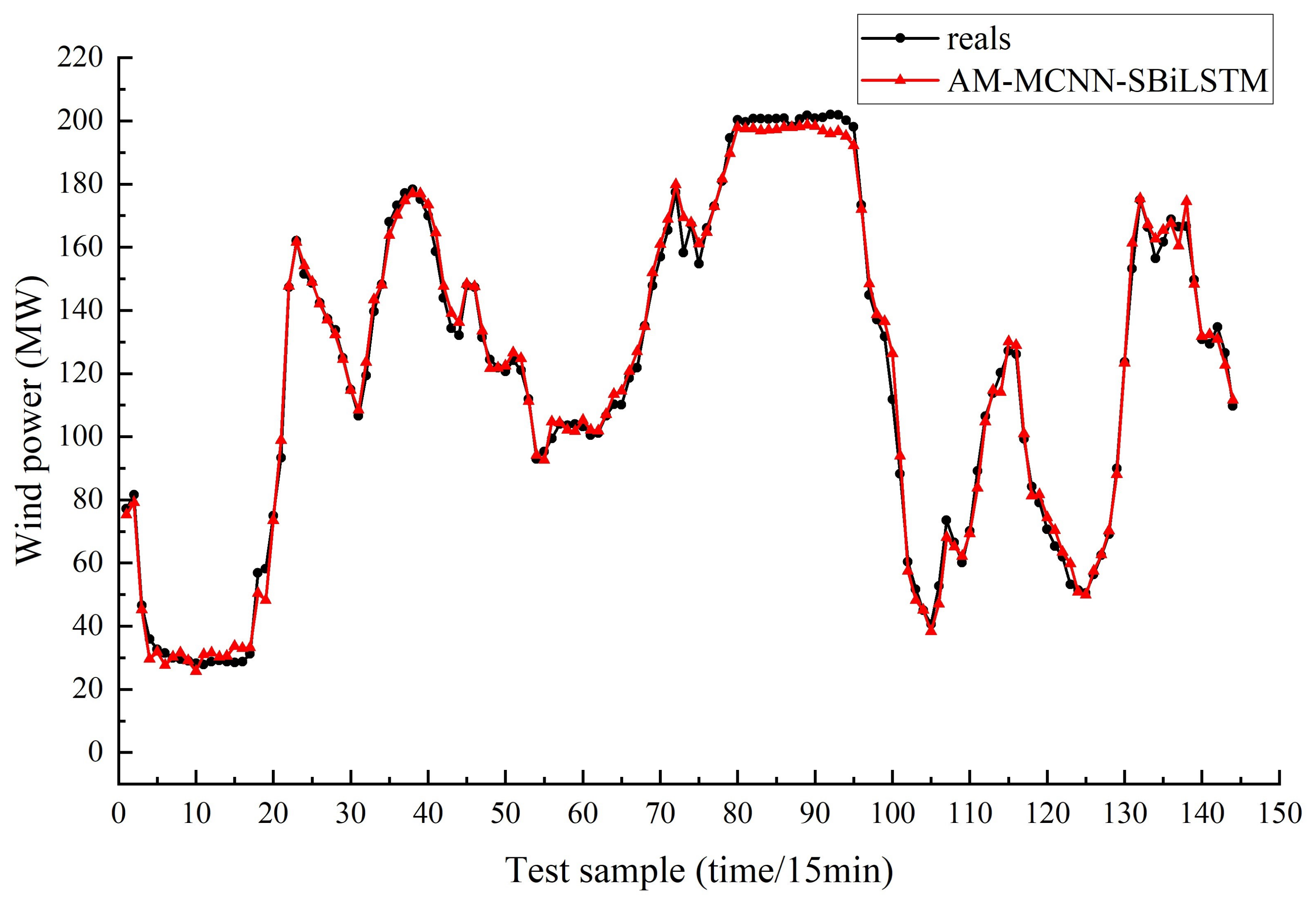
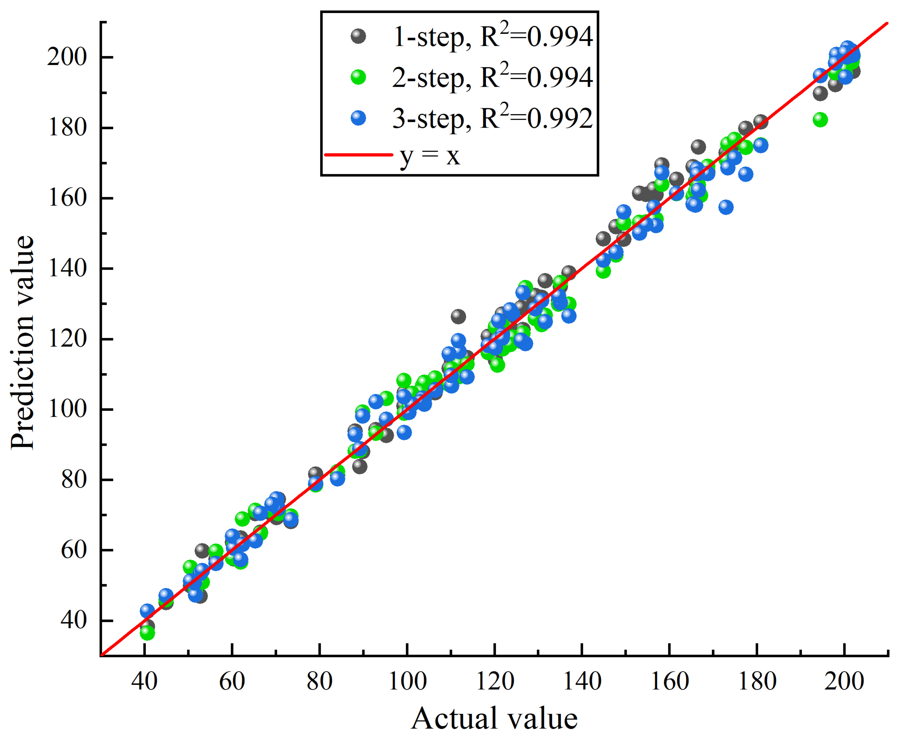
In this work, we propose an AM-MCNN-SBiLSTM prediction model, which utilizes feature weighting and ensemble modeling, for efficient and accurate wind power forecasting. The attention mechanism is used to assign weights to each input feature, effectively addressing the issue where the model fails to discern differences in the importance of input data. The weighted reconstructed feature sequence facilitates the model to extract more key information. By utilizing an MCNN with three types of convolutional kernels and stacking three layers of BiLSTM (SBiLSTM), the model fully explores the multi-scale information of the feature sequence and its long-term trends. Experiments are conducted using actual operational data of wind turbines and compared with the prediction performance of other models. It is demonstrated that the model proposed in this paper exhibits higher predictive accuracy. It demonstrates stronger robustness in experiments with different time steps and longer time ranges and is better able to handle the actual fluctuations of wind power. Thus, this approach can offer more dependable short-term wind power prediction, serving as a reliable point of reference for consistent operation and power allocation in wind farms.

Although the above methods have good predictive performance, their training is complex. We conducted numerous experiments in this study to identify the optimal model parameters, which consumed a significant amount of time. Intelligent algorithms can improve the efficiency of model training. In future research, we plan to use different optimization algorithms to optimize the parameters of the prediction model and to continue to explore the ability of different combination models to extract features, in order to improve prediction accuracy.

References

- Zare, S.G.; Alipour, M.; Hafezi, M.; Stewart, R.A.; Rahman, A. Examining wind energy deployment pathways in complex macro-economic and political settings using a fuzzy cognitive map-based method. Energy 2022, 238, 121673. [Google Scholar] [CrossRef]
- Aslam, M.; Kim, J.-S.; Jung, J. Multi-step ahead wind power forecasting based on dual-attention mechanism. Energy Rep. 2023, 9, 239–251. [Google Scholar] [CrossRef]
- Ullah, T.; Sobczak, K.; Liśkiewicz, G.; Khan, A. Two-dimensional URANS numerical investigation of critical parameters on a pitch oscillating VAWT airfoil under dynamic stall. Energies 2022, 15, 5625. [Google Scholar] [CrossRef]
- Marugán, A.P.; Márquez, F.P.G.; Perez, J.M.P.; Ruiz-Hernández, D. A survey of artificial neural network in wind energy systems. Appl. Energy 2018, 228, 1822–1836. [Google Scholar] [CrossRef]
- Mabel, M.C.; Fernandez, E. Analysis of wind power generation and prediction using ANN: A case study. Renew. Energy 2008, 33, 986–992. [Google Scholar] [CrossRef]
- Niu, D.; Sun, L.; Yu, M.; Wang, K. Point and interval forecasting of ultra-short-term wind power based on a data-driven method and hybrid deep learning model. Energy 2022, 254, 124384. [Google Scholar] [CrossRef]
- Li, L.-L.; Zhao, X.; Tseng, M.-L.; Tan, R.R. Short-term wind power forecasting based on support vector machine with improved dragonfly algorithm. J. Clean. Prod. 2020, 242, 118447. [Google Scholar] [CrossRef]
- Santhosh, M.; Venkaiah, C.; Kumar, D.M.V. Ensemble empirical mode decomposition based adaptive wavelet neural network method for wind speed prediction. Energy Convers. Manag. 2018, 168, 482–493. [Google Scholar] [CrossRef]
- Ma, J.; Yang, M.; Lin, Y. Ultra-short-term probabilistic wind turbine power forecast based on empirical dynamic modeling. IEEE Trans. Sustain. Energy 2020, 11, 906–915. [Google Scholar] [CrossRef]
- Ceyhan, G.; Köksalan, M.; Lokman, B. Extensions for Benders cuts and new valid inequalities for solving the European day-ahead electricity market clearing problem efficiently. Eur. J. Oper. Res. 2022, 300, 713–726. [Google Scholar] [CrossRef]
- Xia, H.; Zheng, J.; Chen, Y.; Jia, H.; Gao, C. Short-term wind speed combined forecasting model based on multi-decomposition algorithms and frameworks. Electr. Power Syst. Res. 2024, 227, 109890. [Google Scholar] [CrossRef]
- Kim, T.-Y.; Cho, S.-B. Predicting residential energy consumption using CNN-LSTM neural networks. Energy 2019, 182, 72–81. [Google Scholar] [CrossRef]
- Dong, X.; Wang, D.; Lu, J.; He, X. A wind power forecasting model based on polynomial chaotic expansion and numerical weather prediction. Electr. Power Syst. Res. 2024, 227, 109983. [Google Scholar] [CrossRef]
- Toubeau, J.-F.; Dapoz, P.-D.; Bottieau, J.; Wautier, A.; Greve, Z.D.; Vallée, F. Recalibration of recurrent neural networks for short-term wind power forecasting. Electr. Power Syst. Res. 2021, 190, 106639. [Google Scholar] [CrossRef]
- Xu, P.; Zhang, M.; Chen, Z.; Wang, B.; Chen, C.; Liu, R. A deep learning framework for day ahead wind power short-term prediction. Appl. Sci. 2023, 13, 4042. [Google Scholar] [CrossRef]
- Karaman, Ö.A. Prediction of wind power with machine learning models. Appl. Sci. 2023, 13, 11455. [Google Scholar] [CrossRef]
- Wang, Y.; Hu, Q.; Meng, D.; Zhu, P. Deterministic and probabilistic wind power forecasting using a variational Bayesian-based adaptive robust multi-kernel regression model. Appl. Energy 2017, 208, 1097–1112. [Google Scholar] [CrossRef]
- Valdivia-Bautista, S.M.; Domínguez-Navarro, J.A.; Pérez-Cisneros, M.; Vega-Gómez, C.J.; Castillo-Téllez, B. Artificial intelligence in wind speed forecasting: A review. Energies 2023, 16, 2457. [Google Scholar] [CrossRef]
- Finamore, A.R.; Calderaro, V.; Galdi, V.; Graber, G.; Ippolito, L.; Conio, G. Improving Wind Power Generation Forecasts: A Hybrid ANN-Clustering-PSO Approach. Energies 2023, 16, 7522. [Google Scholar] [CrossRef]
- Hossain, M.A.; Gray, E.; Lu, J.; Islam, M.R.; Alam, M.S.; Chakrabortty, R.; Pota, H.R. Optimized forecasting model to improve the accuracy of very short-term wind power prediction. IEEE Trans. Ind. Inform. 2023, 19, 10145–10159. [Google Scholar] [CrossRef]
- Jiang, L.; Wang, Y. A wind power forecasting model based on data decomposition and cross-attention mechanism with cosine similarity. Electr. Power Syst. Res. 2024, 229, 110156. [Google Scholar] [CrossRef]
- Xiang, L.; Liu, J.; Yang, X.; Hu, A.; Su, H. Ultra-short term wind power prediction applying a novel model named SATCN-LSTM. Energy Convers. Manag. 2022, 252, 115036. [Google Scholar] [CrossRef]
- Xiao, Y.; Zou, C.; Chi, H.; Fang, R. Boosted GRU model for short-term forecasting of wind power with feature-weighted principal component analysis. Energy 2023, 267, 126503. [Google Scholar] [CrossRef]
- Jalali, S.M.J.; Ahmadian, S.; Khodayar, M.; Khosravi, A.; Shafie-khah, M.; Nahavandi, S.; Catalão, J.P.S. An advanced short-term wind power forecasting framework based on the optimized deep neural network models. Int. J. Electr. Power Energy Syst. 2022, 141, 108143. [Google Scholar] [CrossRef]
- Joseph, L.P.; Deo, R.C.; Prasad, R.; Salcedo-Sanz, S.; Raj, N.; Soar, J. Near real-time wind speed forecast model with bidirectional LSTM networks. Renew. Energy 2023, 204, 39–58. [Google Scholar] [CrossRef]
- Graves, A.; Schmidhuber, J. Framewise phoneme classification with bidirectional LSTM and other neural network architectures. Neural Netw. 2005, 18, 602–610. [Google Scholar] [CrossRef]
- Chen, Q.; He, P.; Yu, C.; Zhang, X.; He, J.; Li, Y. Multi-step short-term wind speed predictions employing multi-resolution feature fusion and frequency information mining. Renew. Energy 2023, 215, 118942. [Google Scholar] [CrossRef]
- Han, Y.; Tong, X.; Shi, S.; Li, F.; Deng, Y. Ultra-short-term wind power interval prediction based on hybrid temporal inception convolutional network model. Electr. Power Syst. Res. 2023, 217, 109159. [Google Scholar] [CrossRef]
- Lv, M.; Wang, J.; Niu, X.; Lu, H. A newly combination model based on data denoising strategy and advanced optimization algorithm for short-term wind speed prediction. J. Ambient Intell. Hum. Comput. 2023, 14, 8271–8290. [Google Scholar] [CrossRef]
- Wang, J.; Lv, M.; Li, Z.; Zeng, B. Multivariate selection-combination short-term wind speed forecasting system based on convolution-recurrent network and multi-objective chameleon swarm algorithm. Expert Syst. Appl. 2023, 214, 119129. [Google Scholar] [CrossRef]
- Zhang, H.; Zhao, L.; Du, Z. Wind power prediction based on CNN-LSTM. In Proceedings of the 2021 IEEE 5th Conference on Energy Internet and Energy System Integration (EI2), Taiyuan, China, 22–24 October 2021; pp. 3097–3102. [Google Scholar] [CrossRef]
- Zhou, B.; Ma, X.; Luo, Y.; Yang, D. Wind power prediction based on LSTM networks and nonparametric kernel density estimation. IEEE Access 2019, 7, 165279–165292. [Google Scholar] [CrossRef]
- Lu, P.; Ye, L.; Pei, M.; Zhao, Y.; Dai, B.; Li, Z. Short-term wind power forecasting based on meteorological feature extraction and optimization strategy. Renew. Energy 2022, 184, 642–661. [Google Scholar] [CrossRef]
- Tang, C.; Lu, J. Research on CNN-LSTM based on attention mechanism for wind power generation prediction. In Proceedings of the 2023 IEEE 3rd International Conference on Data Science and Computer Application (ICDSCA), Dalian, China, 27–29 October 2023; pp. 913–917. [Google Scholar] [CrossRef]
- Luong, M.T.; Pham, H.; Manning, C.D. Effective approaches to attention-based neural machine translation. arXiv 2015, arXiv:1508.04025. [Google Scholar]
- Xiong, B.; Lou, L.; Meng, X.; Wang, X.; Ma, H.; Wang, Z. Short-term wind power forecasting based on Attention Mechanism and Deep Learning. Electr. Power Syst. Res. 2022, 206, 107776. [Google Scholar] [CrossRef]
- Hong, Y.-Y.; Rioflorido, C.L.P.P. A hybrid deep learning-based neural network for 24-h ahead wind power forecasting. Appl. Energy 2019, 250, 530–539. [Google Scholar] [CrossRef]
- Panahi, M.; Sadhasivam, N.; Pourghasemi, H.R.; Rezaie, F.; Lee, S. Spatial prediction of groundwater potential mapping based on convolutional neural network (CNN) and support vector regression (SVR). J. Hydrol. 2020, 588, 125033. [Google Scholar] [CrossRef]
- Goh, H.H.; He, B.; Liu, H.; Zhang, D.; Dai, W.; Kurniawan, T.A.; Goh, K.C. Multi-convolution feature extraction and recurrent neural network dependent model for short-term load forecasting. IEEE Access 2021, 9, 118528–118540. [Google Scholar] [CrossRef]
- Li, J.; Zhang, S.; Yang, Z. A wind power forecasting method based on optimized decomposition prediction and error correction. Electr. Power Syst. Res. 2022, 208, 107886. [Google Scholar] [CrossRef]
- Liang, T.; Zhao, Q.; Lv, Q.; Sun, H. A novel wind speed prediction strategy based on Bi-LSTM, MOOFADA and transfer learning for centralized control centers. Energy 2021, 230, 120904. [Google Scholar] [CrossRef]
- Chen, Y.; Zhao, H.; Zhou, R.; Xu, P.; Zhang, K.; Dai, Y.; Zhang, H.; Zhang, J.; Gao, T. CNN-BiLSTM short-term wind power forecasting method based on feature selection. IEEE J. Radio Freq. Identif. 2022, 6, 922–927. [Google Scholar] [CrossRef]
- Ma, Z.; Mei, G. A hybrid attention-based deep learning approach for wind power prediction. Appl. Energy 2022, 323, 119608. [Google Scholar] [CrossRef]
- Hossain, M.A.; Chakrabortty, R.K.; Elsawah, S.; Ryan, M.J. Very short-term forecasting of wind power generation using hybrid deep learning model. J. Clean. Prod. 2021, 296, 126564. [Google Scholar] [CrossRef]
- Hanifi, S.; Lotfian, S.; Zare-Behtash, H.; Cammarano, A. Offshore wind power forecasting—A new hyperparameter optimisation algorithm for deep learning models. Energies 2022, 15, 6919. [Google Scholar] [CrossRef]
Disclaimer/Publisher’s Note: The statements, opinions and data contained in all publications are solely those of the individual author(s) and contributor(s) and not of MDPI and/or the editor(s). MDPI and/or the editor(s) disclaim responsibility for any injury to people or property resulting from any ideas, methods, instructions or products referred to in the content. |
© 2024 by the authors. Licensee MDPI, Basel, Switzerland. This article is an open access article distributed under the terms and conditions of the Creative Commons Attribution (CC BY) license (https://creativecommons.org/licenses/by/4.0/).