

Rotating Target Detection Using Commercial 5G Signal


Abstract
1. Introduction
2. Related Work
3. 5G Signal and Detection Performance Analysis
3.1. 5G Signal Overview
3.2. Features of 5G Signal Physical Layer
3.2.1. Cyclic Prefix (CP)
3.2.2. Frame Structure
3.2.3. Time–Frequency Resources
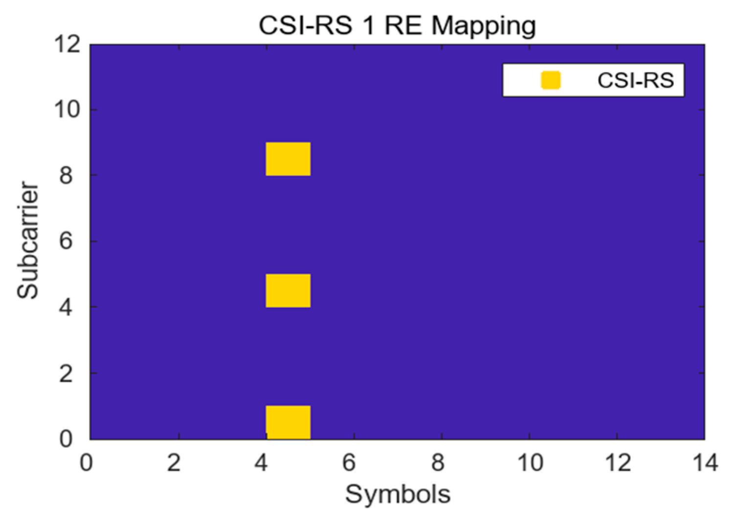
3.3. CSI-RS Signal
4. Target Model and Frequency Offset Extraction Method
4.1. Model Establishment
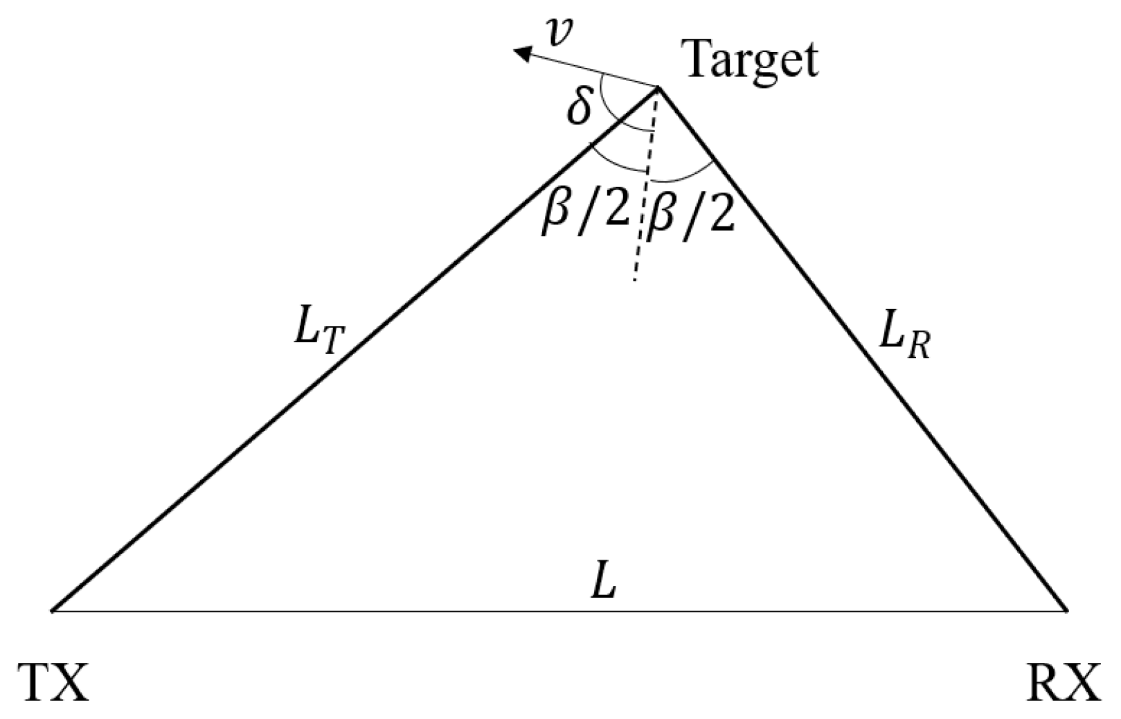
4.1.1. The Bistatic Radar Model
4.1.2. The Model of the Received Signal
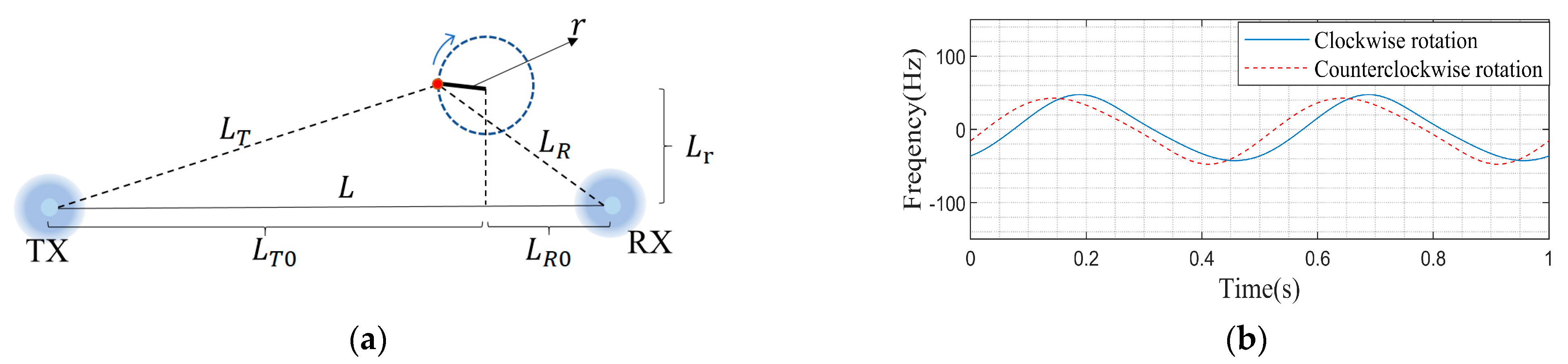
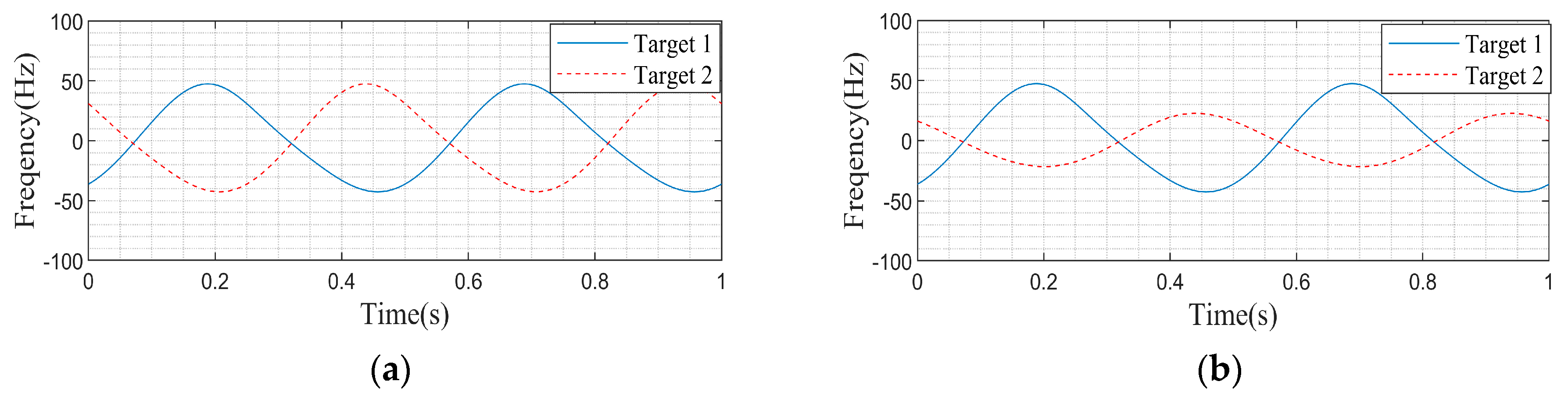
4.1.3. Rotating Target Measurement Scene
- Unilateral rotation target
- 2.
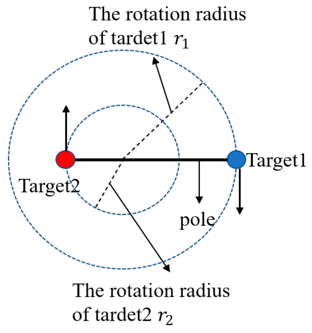
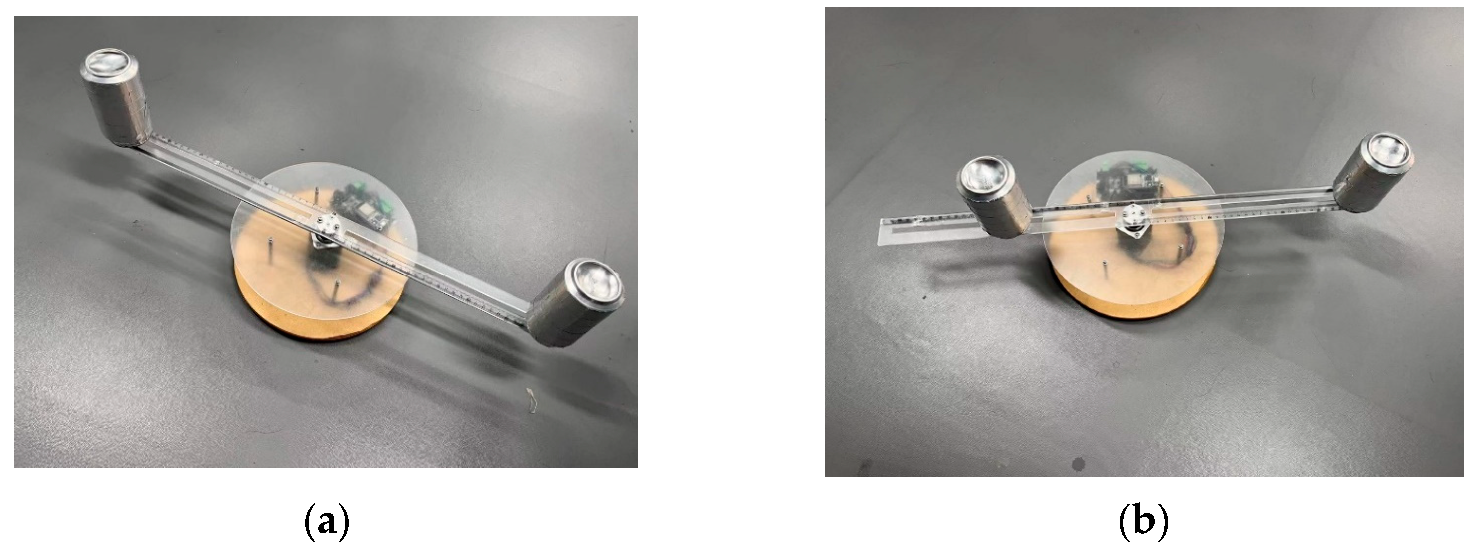
- Bilateral rotating target
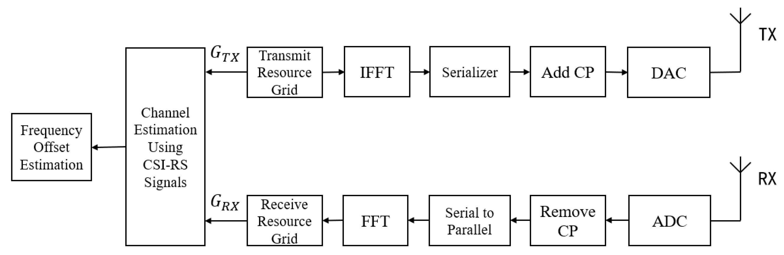
4.2. Target Detection Processing Method
4.2.1. Channel Estimation
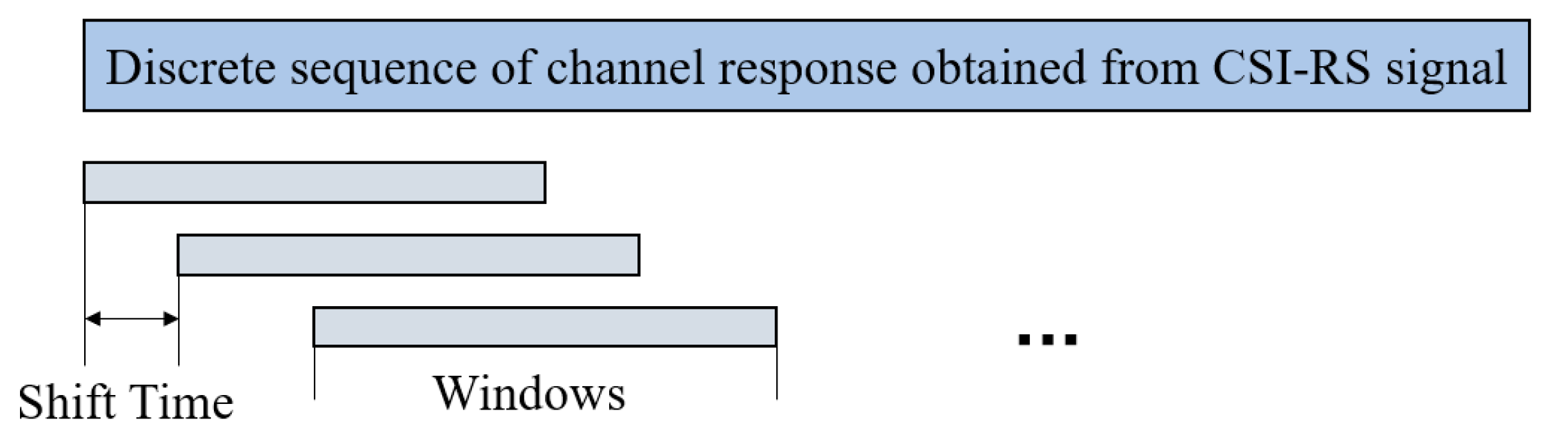
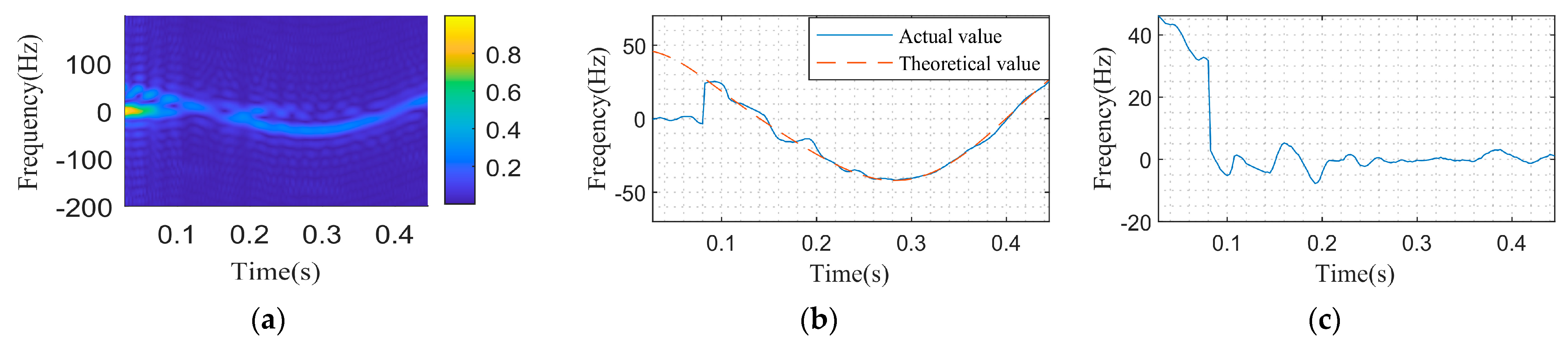
4.2.2. Doppler Frequency Offset Estimation
4.2.3. Interference Suppression
- Direct wave and multipath clutter suppression
- 2.
- Random phase noise suppression
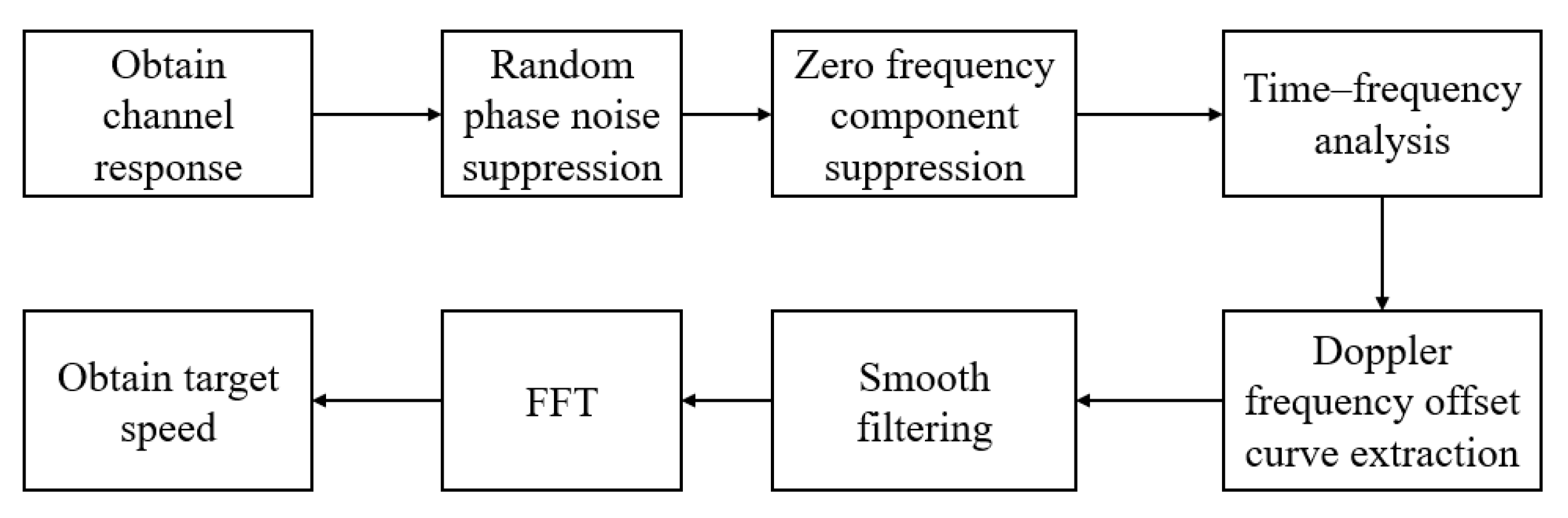
4.3. Summary of Detection Methods
5. Experiments and Data Analysis
5.1. 5G Experimental Base Station Testing
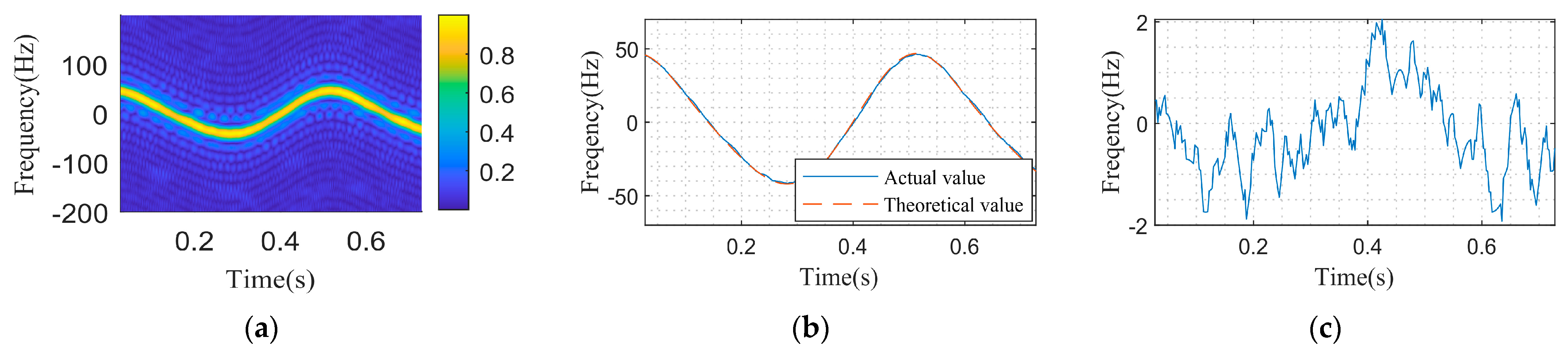
5.1.1. Unilateral Target
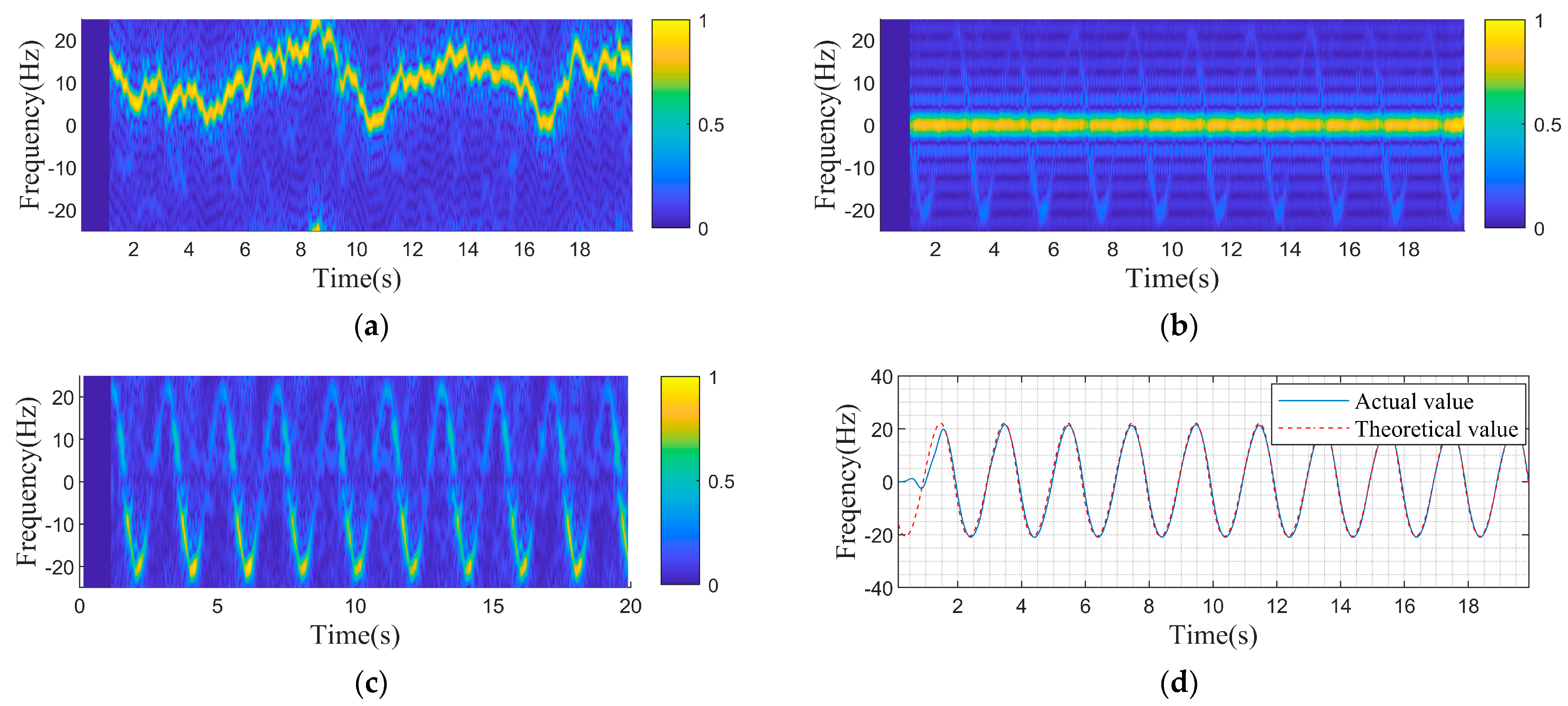
5.1.2. Bilateral Rotating Target
5.2. 5G Commercial Base Station Testing
5.3. Analysis of Computational Load and Processing Time
6. Conclusions
Author Contributions
Funding
Institutional Review Board Statement
Informed Consent Statement
Data Availability Statement
Acknowledgments
Conflicts of Interest
References
- Samczynski, P.; Kulpa, K.; Malanowski, M.; Krysik, P. A concept of GSM-based passive radar for vehicle traffic monitoring. In Proceedings of the 2011 Microwaves, Radar and Remote Sensing Symposium, Kiev, Ukraine, 25–27 August 2011; pp. 271–274. [Google Scholar]
- Falcone, P.; Colone, F.; Bongioanni, C.; Lombardo, P. Experimental results for OFDM WiFi-based passive bistatic radar. In Proceedings of the 2010 IEEE Radar Conference, Arlington, VA, USA, 10–14 May 2010; pp. 516–521. [Google Scholar]
- Colone, F.; Martelli, T.; Bongioanni, C.; Pastina, D.; Lombardo, P. WiFi-based PCL for monitoring private airfields. IEEE Aerosp. Electron. Syst. Mag. 2017, 32, 22–29. [Google Scholar] [CrossRef]
- Wang, B.; Yi, J.; Wan, X.; Dan, Y. Inter-frame ambiguity analysis and suppression of LTE signal for passive radar. J. Radars 2018, 7, 514–522. [Google Scholar]
- Xie, W.; Gan, L.; Shi, C.; Wu, J.; Lee, Y.; Chen, J.; Zhang, R. A Real-time Respiration Monitoring System Using WiFi-Based Radar Model. In Proceedings of the 2022 IEEE International Symposium on Circuits and Systems (ISCAS), Austin, TX, USA, 29 May–1 June 2022; pp. 2082–2086. [Google Scholar]
- Kanhere, O.; Goyal, S.; Beluri, M.; Rappaport, T.S. Target localization using bistatic and multistatic radar with 5G NR waveform. In Proceedings of the 2021 IEEE 93rd Vehicular Technology Conference (VTC2021-Spring), Helsinki, Finland, 25 April–19 May 2021; pp. 1–7. [Google Scholar]
- Księżyk, A.; Płotka, M.; Abratkiewicz, K.; Maksymiuk, R.; Wszołek, J.; Samczyński, P.; Zieliński, T.P. Opportunities and limitations in radar sensing based on 5G broadband cellular networks. IEEE Aerosp. Electron. Syst. Mag. 2023, 38, 4–21. [Google Scholar] [CrossRef]
- Abratkiewicz, K.; Księżyk, A.; Płotka, M.; Samczyński, P.; Wszołek, J.; Zieliński, T.P. Ssb-based signal processing for passive radar using a 5G network. IEEE J. Sel. Top. Appl. Earth Obs. Remote Sens. 2023, 16, 3469–3484. [Google Scholar] [CrossRef]
- Li, X.H. From LTE to 5G Mobile Communication System: Technical Principle and Its LabVIEW Implementation; Tsinghua University Press: Beijing, China, 2020. [Google Scholar]
- Jiang, L.H. 5G NR New Radio Technology Explanation; Publishing House of Electronics Industry: Beijing, China, 2021. [Google Scholar]
- 3GPP TS 38.214: NR, Physical Layer Procedures for Data, 2018. Available online: https://www.etsi.org/deliver/etsi_ts/138200_138299/138214/15.03.00_60/ts_138214v150300p.pdf (accessed on 11 April 2024).
- 3GPP TS 38.211: NR, Physical Channels and Modulation, 2018. Available online: https://www.etsi.org/deliver/etsi_ts/138200_138299/138211/15.02.00_60/ts_138211v150200p.pdf (accessed on 11 April 2024).
- Dahlman, E.; Parkvall, S.; Skold, J. 5GNR: The Next Generation Wireless Access Technology; Elsevier: Amsterdam, The Netherlands, 2018. [Google Scholar]
- 3GPP TS 38.331: NR, Radio Resource Control (RRC) Protocol Specification, 2018. Available online: https://www.etsi.org/deliver/etsi_ts/138300_138399/138331/15.03.00_60/ts_138331v150300p.pdf (accessed on 11 April 2024).
- Núñez-Ortuño, J.M.; González-Coma, J.P.; Nocelo López, R.; Troncoso-Pastoriza, F.; Álvarez-Hernández, M. Beamforming Techniques for Passive Radar: An Overview. Sensors 2023, 23, 3435. [Google Scholar] [CrossRef] [PubMed]
- Samczyński, P.; Abratkiewicz, K.; Płotka, M.; Zieliński, T.P.; Wszołek, J.; Hausman, S.; Korbel, P.; Ksiȩżyk, A. 5G network-based passive radar. IEEE Trans. Geosci. 2021, 60, 1–9. [Google Scholar] [CrossRef]
- Zhao, D.; Wang, J.; Zuo, L.; Wang, J. A Novel Cross-Correlation Algorithm Based on the Differential for Target Detection of Passive Radar. Remote Sens. 2023, 15, 224. [Google Scholar] [CrossRef]
- Li, J.C.; Zhao, Y.D.; Lu, X.D. The impact of step selection in NLMS algorithm on low velocity target detecting for passive radar. In Proceedings of the IET International Radar Conference 2013, Xi’an, China, 14–16 April 2013; pp. 1–4. [Google Scholar]
- Colone, F.; O’hagan, D.; Lombardo, P.; Baker, C.J. A multistage processing algorithm for disturbance removal and target detection in passive bistatic radar. IEEE Trans. Aerosp. Electron. Syst. 2009, 45, 698–722. [Google Scholar] [CrossRef]
- Lyu, X.; Xu, J.; Wang, J. Clutter cancellation in passive radar from the perspective of maximum likelihood. In Proceedings of the 2021 CIE International Conference on Radar (Radar), Haikou, China, 15–19 December 2021; pp. 2808–2811. [Google Scholar]
- Sutar, M.B.; Patil, V.S. LS and MMSE estimation with different fading channels for OFDM system. In Proceedings of the 2017 International Conference of Electronics, Communication and Aerospace Technology (ICECA), Coimbatore, India, 20–22 April 2017; pp. 740–745. [Google Scholar]
- Barneto, C.B.; Anttila, L.; Fleischer, M.; Valkama, M. OFDM radar with LTE waveform: Processing and performance. In Proceedings of the 2019 IEEE Radio and Wireless Symposium (RWS), Orlando, FL, USA, 20–23 January 2019; pp. 1–4. [Google Scholar]
- Reed, I.S.; Gau, Y.-L. A fast CFAR detection space-time adaptive processing algorithm. IEEE Trans. Signal Process. 1999, 47, 1151–1154. [Google Scholar] [CrossRef]
- Meng, X. Rank sum nonparametric CFAR detector in nonhomogeneous background. IEEE Trans. Aerosp. Electron. Syst. 2020, 57, 397–403. [Google Scholar] [CrossRef]
- Wang, Y.; Sun, J. Research on Improving Accuracy of Respiratory Sensing Based on CSI Ratio. In Proceedings of the 2022 2nd International Conference on Computation, Communication and Engineering (ICCCE), Guangzhou, China, 4–6 November 2022; pp. 25–28. [Google Scholar]
- Li, X.; Zhang, J.A.; Wu, K.; Cui, Y.; Jing, X. CSI-ratio-based doppler frequency estimation in integrated sensing and communications. IEEE Sens. J. 2022, 22, 20886–20895. [Google Scholar] [CrossRef]


| Parameter | 4G | 5G NR |
|---|---|---|
| Frequency Range | <3 GHz | FR1: <6 GHz; FR2: >24.25 GHz |
| Subcarrier Spacing | 15 kHz | FR1: 15/30/60 kHz; FR2: 60/120/240 kHz |
| Channel Bandwidth | ≤20 MHz | FR1: ≤100 MHz; FR2: ≤400 MHz |
| Uplink Waveform | DFT-S-OFDM | DFT-S-OFDM/CP-OFDM |
| Downlink Waveform | CP-OFDM | CP-OFDM |
| The Type of Cyclic Prefix | ||
|---|---|---|
| 0 | 15 | Normal |
| 1 | 30 | Normal |
| 2 | 60 | Normal |
| 2 | 60 | Extended |
| 3 | 120 | Normal |
| 4 | 240 | Normal |
| 5 | 480 | Normal |
| 0 | 15 | 10 | 1 | 14 |
| 1 | 30 | 20 | 2 | 14 |
| 2 | 60 | 40 | 4 | 12/14 |
| 3 | 120 | 80 | 8 | 14 |
| 4 | 240 | 160 | 16 | 14 |
| 5 | 480 | 320 | 32 | 14 |
| Parameter | Parameter Value | Parameter | Parameter Value |
|---|---|---|---|
| Num RB | 273 RB | Subcarrier Location | 0 |
| Symbol Locations | 4 | Period | 40 slots |
| Density | 3 | Slot Offset | 24 slots |
| Parameter | Parameter Value | Parameter | Parameter Value |
|---|---|---|---|
| Num RB | 273 RB | Subcarrier Location | 2 |
| Symbol Location | 4 | Period | 40 slots |
| Density | 3 | Slot Offset | 4 slots |
| Theoretical Speed (rps) | Measured Speed (rps) | Error |
|---|---|---|
| 0.125 | 0.122 | 2.4% |
| 0.25 | 0.244 | 2.4% |
| 0.5 | 0.5005 | 0.1% |
| 0.625 | 0.6225 | 0.4% |
| 0.75 | 1.5 | 100% |
| Theoretical Speed (rps) | Measured Speed (rps) | Error |
|---|---|---|
| 0.125 | 0.1221 | 2.3% |
| 0.25 | 0.2563 | 2.5% |
| 0.5 | 0.5005 | 0.1% |
| 0.625 | 0.6226 | 0.38% |
| 0.75 | 0.7568 | 0.9% |
| 0.875 | 0.8789 | 0.45% |
| Step | Number of Floating Point Addition | Number of Floating Point Multiplication | Description |
|---|---|---|---|
| Random phase noise suppression | complex sampling points. | ||
| Zero frequency component suppression | . | ||
| Time–frequency analysis | is length of FFT; is the number of sliding windows. | ||
| Doppler frequency offset curve extraction | \ | Peak search times, with data searched each time. | |
| Smooth filtering | Signal has . | ||
| FFT | . |
Disclaimer/Publisher’s Note: The statements, opinions and data contained in all publications are solely those of the individual author(s) and contributor(s) and not of MDPI and/or the editor(s). MDPI and/or the editor(s) disclaim responsibility for any injury to people or property resulting from any ideas, methods, instructions or products referred to in the content. |
© 2024 by the authors. Licensee MDPI, Basel, Switzerland. This article is an open access article distributed under the terms and conditions of the Creative Commons Attribution (CC BY) license (https://creativecommons.org/licenses/by/4.0/).
Share and Cite
Chen, P.; Tian, L.; Bai, Y.; Wang, J. Rotating Target Detection Using Commercial 5G Signal. Appl. Sci. 2024, 14, 4282. https://doi.org/10.3390/app14104282
Chen P, Tian L, Bai Y, Wang J. Rotating Target Detection Using Commercial 5G Signal. Applied Sciences. 2024; 14(10):4282. https://doi.org/10.3390/app14104282
Chicago/Turabian StyleChen, Penghui, Liuyang Tian, Yujing Bai, and Jun Wang. 2024. "Rotating Target Detection Using Commercial 5G Signal" Applied Sciences 14, no. 10: 4282. https://doi.org/10.3390/app14104282
APA StyleChen, P., Tian, L., Bai, Y., & Wang, J. (2024). Rotating Target Detection Using Commercial 5G Signal. Applied Sciences, 14(10), 4282. https://doi.org/10.3390/app14104282