Weighted Robust Tensor Principal Component Analysis for the Recovery of Complex Corrupted Data in a 5G-Enabled Internet of Things ^†

Abstract

Technological developments coupled with socioeconomic changes are driving a rapid transformation of the fifth-generation (5G) cellular network landscape. This evolution has led to versatile applications with fast data-transfer capabilities. The integration of 5G with wireless sensor networks (WSNs) has rendered the Internet of Things (IoTs) crucial for measurement and sensing. Although 5G-enabled IoTs are vital, they face challenges in data integrity, such as mixed noise, outliers, and missing values, owing to various transmission issues. Traditional methods such as the tensor robust principal component analysis (TRPCA) have limitations in preserving essential data. This study introduces an enhanced approach, the weighted robust tensor principal component analysis (WRTPCA), combined with weighted tensor completion (WTC). The new method enhances data recovery using tensor singular value decomposition (t-SVD) to separate regular and abnormal data, preserve significant components, and robustly address complex data corruption issues, such as mixed noise, outliers, and missing data, with the globally optimal solution determined through the alternating direction method of multipliers (ADMM). Our study is the first to address complex corruption in multivariate data using the WTRPCA. The proposed approach outperforms current techniques. In all corrupted scenarios, the normalized mean absolute error (NMAE) of the proposed method is typically less than 0.2, demonstrating strong performance even in the most challenging conditions in which other models struggle. This highlights the effectiveness of the proposed approach in real-world 5G-enabled IoTs.

1. Introduction

The appearance of fifth-generation (5G) technology, which is capable of integrated communication, presents an excellent opportunity to promote resource management that is informed, sustainable, and robust. This technology provides real-time data on the environmental impacts of different behaviors, opening new possibilities for in-depth analytics. The ability to monitor and control systems quickly has facilitated the creation of intelligent environments. In this context, the Internet of Things (IoT) is expected to emerge as a vital component of 5G applications, particularly in the sensing and monitoring domains [1,2]. The IoT is explicitly designed for massive machine-type communication (mMTC) applications [3], which emphasizes its significance in the changing world of 5G technologies.

The IoT is crucial in various fields ranging from environmental monitoring [4,5,6] to healthcare systems [7,8]. These networks offer a cost-effective means of sensing, collecting, and processing environmental information. However, the deployment of IoTs exposes them to potential data corruption resulting from factors such as device failure, signal interference, and adverse environmental conditions [9]. Consequently, reconstructing corrupt data has become crucial for maintaining the precision and reliability of information collected by IoTs in 5G networks.

A key consideration in addressing the challenges of data reconstruction is gathering real IoT data. Typically, most recently developed WSN appliances utilize sensors with multiple sensing units to detect different variables such as temperature, pressure, O₂, and NO₂ [10]. Therefore, sensor nodes often collect data with multiple attributes, resulting in multivariate data. In addition, the collected data exhibited spatiotemporal and multivariate correlations. The correlations among these attributes can be leveraged to enhance data reconstruction performance. Despite this promising direction, only one work has delved into multivariate data reconstruction in the IoT [11], with limited success.

Using a tensor structure is beneficial for data reconstruction and demonstrates proficiency in harnessing spatiotemporal correlations, particularly for multivariate data. Consequently, traditional methods such as tensor completion (TC) and the tensor robust principal component analysis (TRPCA) [11,12] have been widely employed for both univariate and multivariate data reconstruction. However, these approaches have limitations. They often ignore differences in singular values, treating them uniformly. In the context of data reconstruction, this oversight may result in suboptimal performance.

In practice, the challenges associated with data reconstruction are often complex and involve various forms of corruption, including multiple types of noise, outliers, and missing values. However, previous studies mainly focused on individual types of corruption [11,13]. The corruption of IoT data can occur owing to various factors, including noise, outliers, and missing values. In this study, we consider two types of noise: Gaussian and impulsive. Gaussian noise is a result of hardware imperfections and computational limitations and follows a Gaussian distribution [14]. By contrast, impulsive noise appears suddenly and disrupts information more intensely [15]. It can be triggered by external factors, such as power surges, electromagnetic interference, and faults in sensor nodes, resulting in abrupt changes and extreme data values. Outliers are values that deviate significantly from the normal range. They indicate severe errors in measurements, such as sensor malfunctions, inaccurate readings, and unexpected events in the environment. Outliers are considered abnormal and can significantly affect the overall behavior of data [16]. Missing values are a common issue in IoT data and can occur for various reasons. Sensor nodes may fail to transmit data owing to hardware failures, network problems, or limited energy resources. Environmental conditions, such as signal attenuation or obstacles, can also lead to data loss during transmission [17]. Detecting and addressing these types of data corruption is crucial for ensuring the accuracy and reliability of information in IoTs. IoT academies must learn how to handle these different types of corruption effectively to provide high-quality data for various applications. Previous research focused only on single types of damage, such as Gaussian noise, outliers, and missing values. However, addressing all types of data corruption is essential to ensuring accurate data reconstruction.

This study proposes a new approach to addressing these challenges and makes significant contributions to the field. To the best of our knowledge, this is the first study to address complex corruption encompassing mixed noise, outliers, and missing values in multivariate sensing data within IoTs operating in 5G environments using a WTRPCA. The primary contributions of this study are as follows:

• This work presents an enhanced method for multivariate data reconstruction in 5G-operating IoTs. A TRPCA is combined with TC to enhance the method’s ability to handle missing data, noise, or missing values. This unique approach leverages correlations among multiple attributes to improve reconstruction performance.
• This study introduces a weighted approach to TC and the TRPCA, offering a means of handling singular values. In contrast to traditional methods, the proposed approach uses weighted tensor singular value thresholding (WTSVT) to shrink singular values based on their importance, potentially boosting reconstruction accuracy.
• The proposed approach effectively tackles complex types of corrupted data, such as mixture noise, outliers, and missing values, and stands out in comparison to other models.

This paper is organized as follows: Section 1 introduces the core concepts related to the study, while Section 2 surveys the existing literature and related works on IoTs, TC, and the TRPCA. Section 3 provides the necessary preliminaries, introducing tensors, TC, and the TRPCA in detail. The methodology is presented in Section 4, in which each step of the proposed model is thoroughly explained. An experimental validation of the model, including dataset descriptions, an understanding of the low-rank structure in the dataset, and a description of the experimental setup, is presented in Section 5. Section 6 concludes the paper, summarizes its contributions, and discusses potential directions for future research.

2. Related Work

2.1. Data Reconstruction with Missing Values

The reconstruction of missing data in the IoT is often accomplished using matrix completion algorithms. These algorithms rely on a low-rank matrix to recover missing values by leveraging available spatiotemporal correlations in the data [9,18].

However, these methods have limitations in capturing the complex multivariate relationships inherent in WSN data. These restrictions prevent matrix completion algorithms from fully exploiting multivariate correlations. Utilizing multivariate data enhances the effectiveness of lost data recovery [19,20].

For low-rank data structures, tensor decomposition techniques, particularly tensor singular value decomposition (t-SVD) [21], have been recognized for conserving and leveraging multiattribute correlations. The strength of t-SVD resides in its efficiency, which demands fewer iterations than other decomposition techniques such as CP, Tucker decomposition, and high-order SVD [22,23].

Emerging studies across diverse fields have improved missing data imputation by adopting a unique approach in which the shrinkage of singular values is determined by their importance. This development has been driven by the realization that singular values within the core tensor carry varied importance and should not receive equal treatment during decomposition. Various methodologies have been used to achieve this, including the weighted tensor nuclear norm with t-SVD for TC [24], which is used to restore missing pixels in video and image data. Similarly, the weighted nuclear norm has been applied to unfolded tensors for TC to recover lost data from remote sensing images [25,26]. The weighted tensor nuclear norm for TC uses reconstruction loss data as image data [27].

However, the persistent presence of sparse noise and outliers in data continues to pose a challenge [11]. It is difficult to effectively handle tensor completion because of the effects of sparse noise and outliers. There remains a pressing need for a comprehensive analytical model that focuses on sparse noise and outlier modeling to improve the robustness of IoT data reconstruction address heterogeneously corrupted data complexities.

2.2. Noise and Outlier Reduction Using Robust Principal Component Analysis

At its core, a PCA involves identifying a subspace of a specified dimension that offers an optimal approximation to given data. This is applicable regardless of whether the data are vectors, matrices, or tensors. When applied to data influenced by noise or outliers, the process becomes a robust PCA (RPCA) [28].

Adopting tensor representations and methodologies produces superior results when extracting multidimensional structural features compared with matrix-based approaches. Despite the presence of noise or sparse outliers, this approach to robust tensor data recovery has demonstrated its effectiveness across fields such as SAR imaging [29], hyperspectral image compression [30,31], video sequence background subtraction, image and video denoising [32,33], and wireless communication [34]. With the vast amounts of multi-dimensional data produced by large-scale heterogeneous IoT systems, tensor-based PCAs effectively reveal correlations among multiple attributes. This substantially boosts data reconstruction efficiency in tandem with the recognition of spatiotemporal correlations within individual attributes.

Similar to TC, the TRPCA requires a decomposition method to discover the low-rank structure of data to reduce noise and outliers. Decomposition using t-SVD is computed more efficiently than other methods such as CP decomposition, Tucker decomposition, and high-order SVD (Ho-SVD). Furthermore, t-SVD has been utilized in TRPCAs [23,33].

Similar to TC, discovering the low-rank data structure is essential for reducing noise and outliers in a TRPCA. To achieve this, a decomposition method is required. t-SVD is a more efficient decomposition method than CP decomposition, Tucker decomposition, and Ho-SVD. It is commonly used in TRPCAs [23,33].

It has been observed in various fields that singular values within the RPCA and TRPCA receive weighted shrinkage based on their importance. Several methodologies have been employed to achieve this goal. For instance, a weighted nuclear norm with a truncated SVD was utilized for noise reduction in hyperspectral images [35]. The weighted tensor nuclear norm was used in conjunction with a higher-order RPCA (HoRPCA) for similar purposes [36]. Furthermore, the weighted-tensor p-norm technique, which employs t-SVD, was used to mitigate noise in videos, images [33], and hyperspectral images [37]. These cases highlight the varying shrinkages of singular values based on their importance.

The RPCA and TRPCA aim to recover noise and outliers by identifying low-ranking structures [28]. Therefore, enhancing their ability to manage missing values is essential.

2.3. Primary Challenges in 5G-Enabled IoTs

In the IoT, dealing with noise, outliers, and missing values is a critical area of research. These challenges can have detrimental effects on the accuracy and reliability of collected data. Therefore, it is crucial to investigate and develop solutions to these challenges thoroughly before proceeding with further data exploration. Among the techniques employed to address these challenges, the RPCA can be used often, even though it offers an unsupervised learning approach which is well suited to IoTs. This is primarily because the RPCA does not require labeled data for normal and abnormal classes, a condition that is often challenging to meet in the IoT. However, few recent studies have focused on unsupervised learning, particularly using the RPCA [38].

In addition, research has addressed multivariate data reconstruction, a crucial aspect given the multisensing nature of modern IoT devices [11]. The inclusion of correlations among attributes in multivariate data enhances the accuracy of data reconstruction and anomaly detection, highlighting the need for intensive research in this area [38].

Recent studies have suggested different shrinkages of singular values based on their importance, which is a potential approach for improving data imputation processes [13]. However, a limited number of studies in the literature have exploited this approach for IoTs.

Furthermore, IoTs typically encounter numerous types of noise such as Gaussian and impulsive noise [39,40]. Previous research focused only on a single type of corruption, such as Gaussian noise, outliers, and missing values, without considering other types of corrupted data during data reconstruction. This points to a significant gap in the current knowledge, indicating a strong need for an analytical model to effectively address these complexities.

These challenges highlight the importance of our research on IoTs, which aims to exploit the potential of the RPCA. Our focus includes exploring multivariate data reconstruction, applying different weights to shrink singular values, and addressing a mixed-noise environment encompassing Gaussian noise, impulsive noise, and other corruption types, such as missing values and outliers. This comprehensive approach can significantly boost the robustness and precision of data reconstruction in IoTs.

A summary of research exploring RPCAs, TRPCAs, and our work within the context of noise, outliers, and missing value reconstruction in IoTs is outlined in Table 1. The X in Table 1 indicates that the paper considers the problem.

Table 1. Recent works on RPCA in IoTs.

Paper	Year	Multivariate	Univariate	Corrupted Type				Weighted	Method
				Missing Value	Noise		Outlier
					Gaussian	Impulsive
[11]	2021		X	X	X				TRPCA
[12]	2021	X		X			X		TRPCA-TNN
[13]	2022		X	X	X			X	WRPCA
Our	2024	X		X	X	X	X	X	WRTPCA-WTNN

3. Preliminaries

3.1. Introduction to Tensors

This section briefly introduces the definitions, notation, and tensor operations used in this study. Table 2 lists mathematical symbols, definitions, and commonly used abbreviations.

Table 2. Mathematical notations and definitions.

Notation	Definition
g, g, G, $\mathcal{G}$	scalar, vector, matrix, and tensor formats
${\sigma }_i$	ith singular value
$\mathcal{G}(i,:,:)$, $\mathcal{G}(:,i,:)$, $\mathcal{G}(:,:,i)$	ith horizontal slice, ith lateral slice, and ith frontal slice
${\mathcal{G}}^{\left(i\right)}$	${\mathcal{G}}^{\left(i\right)}=\mathcal{G}(,:,:i)$, ith frontal slice
$\widehat{\mathcal{G}}$	Fourier transformation of $\mathcal{G}$, $\widehat{\mathcal{G}}=fft(\mathcal{G},\left[\right],3)$
${\left|\right|G\left|\right|}_F$	Frobenius norm ${\left|\right|G\left|\right|}_F=\sqrt{{\sum }_{i,j}G{(i,j)}^2}$
${\left|\right|G\left|\right|}_{*}$	nuclear norm ${\left|\right|G\left|\right|}_{*}={\sum }_{i=1}^{min(n_1,n_2)}{\sigma }_i$
${\left|\right|G\left|\right|}_{*,\omega }$	weighted nuclear norm ${\left|\right|G\left|\right|}_{*,\omega }={\sum }_{i=1}^{min(n_1,n_2)}{\sigma }_i{\omega }_i$
${\left|\right|\mathcal{G}\left|\right|}_F$	tensor Frobenius norm ${\left|\right|\mathcal{G}\left|\right|}_F=\sqrt{{\sum }_{i,j,k}\mathcal{G}{(i,j,k)}^2}$
${\left|\right|\mathcal{G}\left|\right|}_{*}$	tensor nuclear norm ${\parallel \mathcal{G}\parallel }_{*}={\sum }_{j=1}^{n_3}{\sum }_{i=1}^{min(n_1,n_2)}{\sigma }_{ij}$
${\left|\right|\mathcal{G}\left|\right|}_{*,\omega }$	weighted tensor nuclear norm ${\left|\right|\mathcal{G}\left|\right|}_{*,\omega }={\sum }_{j=1}^{n_3}{\sum }_{i=1}^{min(n_1,n_2)}{\sigma }_{ij}{\omega }_{ij}$
$rank\left(G\right)$	rank of matrix G
$rank\left(\mathcal{G}\right)$	tubal rank of tensor $\mathcal{G}$
t-SVD	tensor singular value decomposition
ADMM	alternative direction method of multipliers
WTNN	weighted tensor nuclear norm
$\mathsf{\Omega }$	position of missing elements in $\mathcal{G}$
${\mathcal{P}}_{\mathsf{\Omega }}$	projection on $\mathsf{\Omega }$

$\mathcal{G}\in {\mathbb{R}}^{n_1\times n_2\times n_3...\times n_N}$ represents a multiway array of the Nth order, also referred to as an N-way array or Nth-order tensor. In a specific instance in which N = 3, $\mathcal{G}\in {\mathbb{R}}^{n_1\times n_2\times n_3}$ is defined as a third-order tensor. A slice is a data partition that occurs when one mode index is fixed, whereas the indices in the other two modes vary. The slices of a third-order tensor are illustrated in Figure 1. Fibers of the third-order tensor were obtained by maintaining all except one dimension constant, as shown in Figure 2.

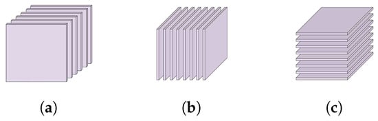
Figure 1. Slices of third-order tensor $\mathcal{G}$: (a) frontal slices; (b) lateral slices; (c) horizontal slices.

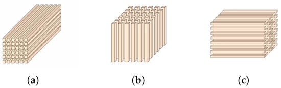
Figure 2. Fibers of third-order tensor $\mathcal{G}$: (a) tube fibers; (b) column fibers; (c) row fibers.

For the tensor $\mathcal{G}\in {\mathbb{R}}^{n_1\times n_2\times n_3}$, the ith frontal slices are indicated by ${\mathcal{G}}^{\left(i\right)}$, where i ranges from one to $n_3$. The operation $unfold$ is described as follows:

$$unfold\left(\mathcal{G}\right)=\left[\begin{array}{c}{G}^{\left(1\right)}\\ G^{\left(2\right)}\\ ⋮\\ G^{\left(n_3\right)}\end{array}\right]$$

(1)

Furthermore, the $fold$ operation is as follows:

$$fold\left(\left[\begin{array}{c}{G}^{\left(1\right)}\\ G^{\left(2\right)}\\ ⋮\\ G^{\left(n_3\right)}\end{array}\right]\right)=\mathcal{G}$$

(2)

The block circulant matricization operator, denoted by $circ$, was defined in [21]. This operator reshapes tensor $\mathcal{G}\in {\mathbb{R}}^{n_1\times n_2\times n_3}$ into a block circulant matrix of size $G\in {\mathbb{R}}^{n_1{n}_3\times n_2{n}_3}$. The block circulant matricization operator arranges the frontal slices of tensor A in a circulant manner, thereby preserving the temporal relationships across the frontal slices and the multivariate correlations within the frontal slices.

$$circ\left(\mathcal{G}\right)=\left[\begin{array}{cccc}{G}^{\left(1\right)}& G^{\left(n_3\right)}& \cdots & G^{\left(2\right)}\\ G^{\left(2\right)}& G^{\left(1\right)}& \cdots & G^{\left(3\right)}\\ ⋮& ⋮& ⋮& ⋮\\ G^{\left(n_3\right)}& G^{(n_3-1)}& \cdots & G^{\left(1\right)}\end{array}\right]$$

(3)

Within the tensor–SVD framework, the tensor product is conceptualized as an extension of the matrix product.

Definition 1. 

The tensor product [21] involves two tensors, $\mathcal{G}\in {\mathbb{R}}^{n_1\times n_2\times n_3}$ and $\mathcal{Y}\in {\mathbb{R}}^{n_1\times n_4\times n_3}$. The t-product, represented by $\mathcal{G}\ast \mathcal{Y}$, is defined as a tensor of size $n_1\times n_4\times n_3$. This is given by

$$\mathcal{G}\ast \mathcal{Y}=fold\left(circ\right(\mathcal{G})·(unfold\left(\mathcal{Y}\right))$$

(4)

Definition 2. 

A conjugate transpose, as detailed in [21], involves a tensor $\mathcal{G}\in {\mathbb{R}}^{n_1\times n_2\times n_3}$. The conjugate transpose of this tensor, denoted by ${\mathcal{G}}^{★}\in {\mathbb{R}}^{n_2\times n_1\times n_3}$, is obtained by taking the conjugate transpose of each frontal slice and subsequently reversing the order of the transposed frontal slices from 2 to $n_3$.

Definition 3. 

An identity tensor  [21] is a tensor $\mathcal{G}\in {\mathbb{R}}^{n_1\times n_2\times n_3}$. This tensor is characterized by its first frontal slice being an $n\times n$ identity matrix, whereas all other frontal slices consist entirely of zeros.

Definition 4. 

A block diagonal matrix  [41] with $\widehat{\mathcal{G}}=fft\left(\mathcal{G}\right)$ represents the tensor obtained by executing a fast Fourier transform (FFT) along the third dimension of the tensor $\mathcal{G}\in {\mathbb{R}}^{n_1\times n_2\times n_3}$. The block diagonal matrix of $\widehat{\mathcal{G}}$ is defined as follows:

$$\widehat{G}=blockdiag\left(\widehat{\mathcal{G}}\right)=\left[\begin{array}{cccc}{G}^{\left(1\right)}& & & 0\\ & G^{\left(2\right)}& & \\ & & \ddots & \\ 0& & & G^{\left(n_3\right)}\end{array}\right]$$

(5)

Definition 5. 

An orthogonal tensor [21] is a tensor $\mathcal{G}\in {\mathbb{R}}^{n_1\times n_1\times n_3}$. This tensor is considered orthogonal if it fulfills the following condition:

$$\mathcal{G}\ast {\mathcal{G}}^T={\mathcal{G}}^T\ast \mathcal{G}=\mathcal{I}$$

(6)

Definition 6. 

$\mathit{f}\mathbf{-}$diagonal tensor  [21] is a tensor $\mathcal{G}\in {\mathbb{R}}^{n_1\times n_1\times n_3}$. This tensor is considered orthogonal if it satisfies the following conditions.

Theorem 1. 

Tensor Singular Value Decomposition (t-SVD) [21] is a method of decomposing a third-order tensor. It breaks down a tensor $\mathcal{G}\in {\mathbb{R}}^{n_1\times n_2\times n_3}$ into three components: a core tensor $\mathcal{D}\in {\mathbb{R}}^{n_1\times n_1\times n_3}$, an orthogonal tensor on the right $\mathcal{U}\in {\mathbb{R}}^{n_1\times n_1\times n_3}$, and an orthogonal tensor on the left $\mathcal{V}\in {\mathbb{R}}^{n_2\times n_2\times n_3}$. The decomposition is expressed as follows:

$$\mathcal{G}=\mathcal{U}\ast \mathcal{D}\ast {\mathcal{V}}^T$$

(7)

In the t-SVD process for a third-order tensor, as illustrated in Algorithm 1, tensor $\mathcal{G}\in {\mathbb{R}}^{n_1\times n_2\times n_3}$ is decomposed into three distinct tensors. $\mathcal{U}$ and $\mathcal{V}$ are orthogonal tensors, whereas $\mathcal{D}$ is an $f-$diagonal core tensor. Each frontal slice of the core tensor $\mathcal{D}$ is a diagonal matrix, as shown in Figure 3.

Algorithm 1 Tensor singular value decomposition (t-SVD).

1: Input: $\mathcal{G}\in {\mathbb{R}}^{n_1\times n_2\times n_3}$ 2: $\mathcal{P}=\mathrm{fft}(\mathcal{G},[],3)$ 3: for $i=1$ to $n_3$ do 4:    $\mathit{[}\mathit{U},\mathit{D},\mathit{V}\mathit{]}=\mathit{SVD}(\mathcal{G}(:,:,\mathrm{i}))$ 5:    Determine frontal slices of U, D, and V 6:    $\widehat{\mathcal{U}}(:,:,i)$ = $\mathbf{U}$ 7:    $\widehat{\mathcal{D}}(:,:,i)$ = $\mathbf{D}$ 8:    $\widehat{\mathcal{V}}(:,:,i)$ = $\mathbf{V}$ 9: end for 10: U = $ifft(\widehat{\mathcal{U}},\left[\right],3)$, D = $ifft(\widehat{\mathcal{D}},\left[\right],3)$, V = $ifft(\widehat{\mathcal{V}},\left[\right],3)$ 11: Output: orthogonal tensor $\mathcal{U}$, $\mathcal{D}$ and core tensor $\mathcal{V}$

Figure 3. Tensor singular value decomposition (t-SVD).

Definition 7. 

The tubal rank  [41] is the count of non-zero singular tubes present in the core tensor $\mathcal{D}$, which is derived from the t-SVD of $\mathcal{G}\in {\mathbb{R}}^{n_1\times n_2\times n_3}$.

Definition 8. 

The tensor nuclear norm [42], denoted ${\parallel ·\parallel }_{*}$ of tensor $\mathcal{G}\in {\mathbb{R}}^{n_1\times n_2\times n_3}$, is the mean value of the nuclear norm of all frontal slices of the tensor $\widehat{\mathcal{G}}$.   

$${\parallel \mathcal{G}\parallel }_{*}=\frac{1}{n_3}{∥\widehat{\mathcal{G}}∥}_{*}=\frac{1}{n_3}\sum _{j=1}^{n_3}\sum _{i=1}^{min(n_1,n_2)}{\sigma }_{ij}$$

(8)

Definition 9. 

The weighted tensor nuclear norm [24], represented as ${\parallel ·\parallel }_{*,\omega }$ of tensor $\mathcal{G}\in {\mathbb{R}}^{n_1\times n_2\times n_3}$, is the mean value of the weighted nuclear norm of all frontal slices of tensor $\widehat{\mathcal{G}}$ given that $\omega \ge 0$.

$${∥\mathcal{G}∥}_{*,\omega }=\frac{1}{n_3}\sum _{j=1}^{n_3}\sum _{i=1}^{min(n_1,n_2)}{\omega }_{ij}{\sigma }_{ij}$$

(9)

3.2. Tensor Robust Principal Component Analysis with Weighted Tensor Nuclear Norm Minimization

The RPCA is designed to accurately separate a low-rank matrix $\mathit{L}$ and a sparse matrix $\mathit{C}$ from a corrupted matrix $\mathit{G}\in {\mathbb{R}}^{n_1\times n_2}$. A direct solution to this problem is as follows:

$${\min }_{\mathit{L},\mathit{C}}rank\left(L\right)+\lambda {\parallel C\parallel }_0,\mathrm{s}.\mathrm{t}.G=L+C,$$

(10)

Here, the ${\ell }_0$-norm is denoted by ${\parallel ·\parallel }_0$, and the weight-adjusting parameter $\lambda$ is positive. The rank of the matrix is presented by $rank(·)$. Equation (10) represents the matrix rank minimization, which is a non-convex and NP-hard problem. A more feasible approach to the low-rank matrix reconstruction problem is to minimize a weighted linear combination of the matrix nuclear norm and the ${\ell }_1$-norms [28]. The approach is as follows:

$${\min }_{\mathit{L},\mathit{C}}{\parallel L\parallel }_{*}+\lambda {\parallel C\parallel }_1,\mathrm{s}.\mathrm{t}.G=L+C$$

(11)

In Equation (11), ${\left|\right|L\left|\right|}_{*}={\sum }_{i=1}^{min(n_1,n_2)}{\sigma }_i$ is the matrix nuclear norm, and ${\sigma }_i$ is the $i_{th}$ singular value of $\mathit{L}$. The ${\ell }_1$-norm is denoted as ${\parallel ·\parallel }_1$. Introducing the weighted nuclear norm allows different singular values to shrink differently, thereby preserving major data components [43]. This is expressed as follows:

$${\min }_{\mathit{L},\mathit{C}}{\parallel L\parallel }_{*,\omega }+\lambda {\parallel C\parallel }_1,\mathrm{s}.\mathrm{t}.G=L+C$$

(12)

In Equation (12), ${\left|\right|L\left|\right|}_{*,\omega }={\sum }_{i=1}^{min(n_1,n_2)}{\sigma }_i{\omega }_i$ is the weighted nuclear norm (WNN), and $\omega \ge 0$ is the weight parameter. Additionally, the RPCA is expanded to handle multi-dimensional data while maintaining the tensor structure via the TRPCA. This technique has been effective in several fields including image processing, background removal, and image reconstruction. It has proven particularly useful in addressing noise damage issues in IoTs. As shown in Figure 4, the TRPCA is used to restore low-rank tensors damaged by sparse noise. The different colors present different columns or attributes in the data tensor.

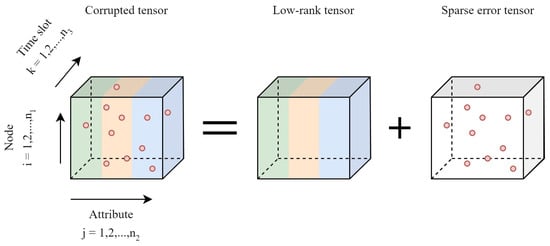
Figure 4. Decomposition of low-rank and sparse components from corrupted TRPCA observation.

The weighted tensor nuclear norm (WTNN) minimization for the TPRCA [44] is given as follows:

$$\begin{array}{c}{\min }_{\mathcal{L},\mathcal{C}}\Vert \mathcal{L}{\Vert }_{*,\omega }+\lambda \Vert \mathcal{C}{\Vert }_1,\mathrm{s}.\mathrm{t}.\mathcal{G}=\mathcal{L}+\mathcal{C}\hfill \end{array}$$

(13)

where ${\left|\right|\mathcal{L}\left|\right|}_{*,\omega }={\sum }_{j=1}^{n_3}{\sum }_{i=1}^{min(n_1,n_2)}{\sigma }_{ij}{\omega }_{ij}$, the weight parameters, are arranged such that a more significant singular value is paired with a smaller weight and vice versa. This configuration ensures equal treatment of all singular values within the objective function. Following this, the weight parameters were initialized and fixed in non-decreasing order as follows: $0\le {\omega }_1\le {\omega }_2\le ...\le {\omega }_{min(n_1,n_2)}$.

3.3. Tensor Completion with Weighted Tensor Nuclear Norm Minimization

The matrix completion (MC) model aims to estimate missing values based on incomplete observations. This model can be represented by the following equation [45]:

$$\begin{array}{c}{\min }_{\mathrm{A}}rank\left(A\right),\mathrm{s}.\mathrm{t}.{\mathcal{P}}_{\mathsf{\Omega }}\left(A\right)={\mathcal{P}}_{\mathsf{\Omega }}\left(B\right)\hfill \end{array}$$

(14)

In Equation (14), $A\in {\mathbb{R}}^{n_1\times n_2}$ represents the matrix, $\mathsf{\Omega }$ indicates the support set, ${\mathcal{P}}_{\mathsf{\Omega }}$ is the orthogonal projection onto the span of the matrices, and the values of the matrices disappear outside of $\mathsf{\Omega }$. Therefore, the ${(i,j)}_{th}$ component of ${\mathcal{P}}_{\mathsf{\Omega }}\left(A\right)$ equals $B_{ij}$ if the ${(i,j)}_{th}$ component $\in \mathsf{\Omega }$ and is zero otherwise. Given the NP-hard complexity of minimizing the matrix rank, the nuclear norm minimization problem offers an effective approximation of the MC model [45]:

$$\begin{array}{c}{\min }_{\mathrm{A}}{\left|\right|A\left|\right|}_{*}\mathrm{s}.\mathrm{t}.{\mathcal{P}}_{\mathsf{\Omega }}\left(A\right)={\mathcal{P}}_{\mathsf{\Omega }}\left(B\right)\hfill \end{array}$$

(15)

In Equation (15), ${\left|\right|A\left|\right|}_{*,\omega }={\sum }_{i=1}^{min(n_1,n_2)}{\sigma }_i{\omega }_i$ represents the nuclear norm of the matrix, where ${\sigma }_i$ is the $i_{th}$ singular value of A. Nevertheless, this approximation does not adequately account for the most and least significant singular values. An improved solution is the weighted nuclear norm, which assigns higher weights to less significant singular values and lower weights to more significant ones [46]:

$$\begin{array}{c}{\min }_{\mathrm{A}}{\left|\right|A\left|\right|}_{*,\omega }\mathrm{s}.\mathrm{t}.{\mathcal{P}}_{\mathsf{\Omega }}\left(A\right)={\mathcal{P}}_{\mathsf{\Omega }}\left(B\right)\hfill \end{array}$$

(16)

where ${\left|\right|A\left|\right|}_{*,\omega }={\sum }_{i=1}^{min(n_1,n_2)}{\sigma }_i{\omega }_i$ is the WNN, and $\omega \ge 0$ is the weight parameter. Tensor completion, a multi-dimensional extension of matrix completion, is depicted in Figure 5. The data tensor’s various colors correspond to distinct columns or properties.

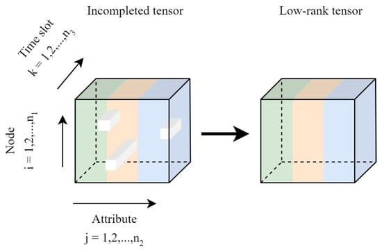
Figure 5. Missing and low-rank components of TC.

WTNN minimization for TC was proposed in [24] and can be expressed as follows:

$$\begin{array}{c}{\min }_{\mathcal{A}}{\left|\right|\mathcal{A}\left|\right|}_{*,\omega }\mathrm{s}.\mathrm{t}.{\mathcal{P}}_{\mathsf{\Omega }}\left(\mathcal{A}\right)={\mathcal{P}}_{\mathsf{\Omega }}\left(\mathcal{B}\right)\hfill \end{array}$$

(17)

4. The Proposed Model

Many studies regarding IoT data corruption have not taken into account all the different types of corruption that can occur. In this proposed model, we use a combination of the WRTPCA and WTC. The input data for this method comprise a tensor that has been damaged with missing values, mixed noise, and outliers. We apply WTSVT (Algorithm 2) in both WTC and the WRTPCA. WTC (Algorithm 3) results in a new tensor that has no missing values. This new tensor is then input into the WRTPCA (Algorithm 4). After applying this proposed model, we obtain a final tensor that has no missing values, mixture noise, or outliers. Figure 6 provides an overview of this proposed model. Before discussing the details of this method, we present the mathematical foundations of WTC and the WRTPCA.

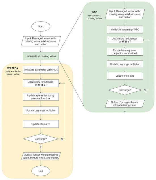
Figure 6. Flowchart of our model—WRTPCA integrated with WTC.

To recover the missing-value tensor, Equation (17) can be solved to extract the low-rank structure from the incomplete tensor data using the alternating direction method of multipliers (ADMMs) [24] as follows:

$${\widehat{\mathcal{W}}}_{i+1}=arg\underset{\widehat{\mathcal{W}}}{min}\left(\right||\widehat{\mathcal{W}}{\left|\right|}_{*,\omega }-\frac{{\beta }_i}{2}\parallel \widehat{\mathcal{W}}-{\widehat{\mathcal{A}}}_i-\frac{1}{{\beta }_i}{\widehat{\mathcal{U}}}_i{\parallel }_{\mathrm{F}}^2)$$

(18)

$$\begin{array}{c}\hfill {\mathcal{A}}_{i+1}=arg\underset{\mathcal{A}}{min}({\delta }_{\mathcal{Y}={\mathcal{P}}_{\mathsf{\Omega }}\left(\mathbf{X}\right)}+⟨\mathcal{U}(:),\mathcal{A}(:)⟩\\ \hfill +\frac{{\beta }_i}{2}{∥\mathcal{A}-{\mathcal{W}}_{i+1}∥}_F^2)\end{array}$$

(19)

$${\mathcal{U}}_{i+1}={\mathcal{U}}_i+{\beta }_i({\mathcal{A}}_{i+1}-{\mathcal{W}}_{i+1})$$

(20)

The WRTPCA optimization model, depicted in Equation (13), is frequently resolved by employing the ADMM [33]. The solution to the low-rank optimization problem can be expressed as follows:

$${\mathcal{L}}_{i+1}=arg\underset{\mathcal{L}}{min}{\left(\right|\left|\mathcal{L}\right||}_{*,\omega }+\frac{{\mu }_i}{2}\parallel \mathcal{L}-\mathcal{G}+{\mathcal{C}}_i-\frac{{\mathcal{Y}}_i}{{\mu }_i}{\parallel }_{\mathrm{F}}^2)$$

(21)

$${\mathcal{C}}_{i+1}=arg\underset{\mathcal{C}}{min}{\left(\lambda \right|\left|\mathcal{C}\right||}_1+\frac{{\mu }_i}{2}\parallel {\mathcal{L}}_{i+1}-\mathcal{G}+\mathcal{C}-\frac{{\mathcal{Y}}_i}{{\mu }_i}{\parallel }_{\mathrm{F}}^2)$$

(22)

$${\mathcal{Y}}_{i+1}={\mathcal{Y}}_i+{\mu }_i({\mathcal{L}}_{i+1}+{\mathcal{C}}_{i+1}-\mathcal{G})$$

(23)

Algorithm 2 Weighted tensor singular value thresholding method ($\mathbf{WTSVT}$).

1: Input: $\mathcal{M}\in {\mathbb{R}}^{n_1\times n_2\times n_3},\beta$, $\omega$ 2: $\mathcal{F}=\mathrm{fft}(\mathcal{M},[],3)$ 3: for $i=1$ to $n_3$ do 4:    $\mathit{[}\mathit{U},\mathit{D},\mathit{V}\mathit{]}=\mathrm{SVD}(\mathcal{F}(:,:,\mathrm{i}))$ 5:    $diagD=diag\left(\mathbf{D}\right)-\frac{\omega }{\beta }$ 6:    $\mathbf{ddiagD}$ = $diag\left(diagD\right)$ 7:    $\widehat{\mathcal{U}}(:,:,i)$ = $\mathbf{U}$ 8:    $\widehat{\mathcal{D}}(:,:,i)$ = $\mathbf{ddiagD}$ 9:    $\widehat{\mathcal{V}}(:,:,i)$ = $\mathbf{V}$ 10: end for 11: U= $ifft(\widehat{\mathcal{U}},\left[\right],3)$, D= $ifft(\widehat{\mathcal{D}},\left[\right],3)$, V= $ifft(\widehat{\mathcal{V}},\left[\right],3)$ 12: Output: orthogonal tensor $\mathcal{U}$, $\mathcal{D}$ and core tensor $\mathcal{V}$

Weighted tensor singular value thresholding (WTSVT), with a threshold based on the weighted tensor nuclear norm (WTNN), employs t-SVD [24], which solves the drawbacks of using a fixed threshold for each singular value. Equations (18) for TC and (21) in the TRPCA are solved using WTSVT. This method helps recover missing values in the TC and minimizes noise and outliers in the TRPCA [33]. To maintain essential data components, WTSVT is used to optimize the low-rank tensor $\mathcal{L}$. WTSVT calculates the total weighted singular values over all the frontal slices of the tensor data, ensuring that greater singular values decrease less. In Algorithms 3 and 4, the WTSVT operator is used, and it is defined in Algorithm 2. The objective of Algorithm 2 is to break down the input tensor into three tensors, with the middle tensor being a low-rank tensor. The inputs for WTSVT include the input tensor $\mathcal{M}$ and the weighted vector $\omega$, and $\beta$ is the penalty factor. The notation $fft$ represents the FFT used to compute the discrete Fourier transform (DFT) of a sequence. In contrast, $ifft$ represents the inverse fast Fourier, which essentially reverses the FFT process. First, the input tensor is transformed using $fft$. Next, the loop of Algorithm 2 begins, and each frontal slice of the input tensor is applied ($SVD$). The process $SVD$ breaks down a matrix into three separate matrices—a left singular matrix, a diagonal matrix of singular values, and a matching singular matrix. The $diag$ pertains to the diagonal elements of the singular matrix. The operation $diag\left(\mathbf{D}\right)-\frac{\omega }{\beta }$ takes each diagonal component, converts it into a vector, and subtracts it, with each value in vector $\omega$ already divided to $\beta$. Subsequently, the $diag\left(diagD\right)$ converts $diagD$ into a diagonal matrix with shrunken singular values. The weight shrinks the diagonal elements in the singular matrix D. After completing $SVD$ for all frontal slices, $ifft$ is used with the three components to obtain results.

Algorithm 3 Weighted tensor completion.

Input: $\mathcal{B}\in {\mathbb{R}}^{n_1\times n_2\times n_3}$ with missing values, weighted vector $\omega$ Initialize: ${\mathcal{A}}_0=\mathcal{B}$, ${\mathcal{W}}_0=\mathcal{B}$, ${\mathcal{U}}_0=\mathcal{O}$, $ϵ=1\times {10}^{-8}$, $\rho =1.1$, ${\beta }_0=1\times {10}^{-1}$ while not converged do    Update ${\widehat{\mathcal{W}}}_{i+1}$ = $\mathbf{WTSVT}$$(\widehat{{\mathcal{A}}_i}+\frac{{\widehat{\mathcal{U}}}_i}{{\beta }_i},\omega ,{\beta }_i)$    Update ${\mathcal{A}}_{i+1}={\mathcal{W}}_{i+1}-\frac{1}{{\mathcal{Z}}_i}{\mathcal{U}}_i$, ${\mathcal{P}}_{\mathsf{\Omega }}\left({\mathcal{A}}_{i+1}\right)={\mathcal{P}}_{\mathsf{\Omega }}\left(\mathcal{B}\right)$    Update ${\mathcal{U}}_{i+1}={\mathcal{U}}_i+{\beta }_i({\mathcal{A}}_{i+1}-{\mathcal{W}}_{i+1})$    Update ${\beta }_{i+1}=$$\rho$${\beta }_i$    Check the convergence criteria $\parallel {\mathcal{A}}_{i+1}-{\mathcal{W}}_i{\parallel }_F^2\le ϵ$ or $\parallel {\mathcal{A}}_i-{\mathcal{A}}_{i+1}{\parallel }_F^2\le ϵ$ or $\parallel {\mathcal{W}}_i-{\mathcal{W}}_{i+1}{\parallel }_F^2\le ϵ$ end while Output: low-rank tensor without missing value $\mathcal{A}$

The solution to Equation (18) is obtained through WTSVT (Algorithm 2), and Equation (19) represents the least-squares projection constrained by the problem [42]. The $\delta$-indicator function maps the elements of a subset of a set to one and all other elements to zero. Following MATLAB R2021a notation, the symbols $\mathcal{U}(:)$ and $\mathcal{G}(:)$ signify the tensor-to-vector conversion. To recover the missing values, the ADMM is implemented, the details of which are provided in Algorithm 3. The input to Algorithm 3 includes a tensor with the missing values $\mathcal{B}$ and weighted vector $\omega$. First, we initialize the tensors $\mathcal{A}$, $\mathcal{W}$, and $\mathcal{U}$ as $\mathcal{B}$, $\mathcal{B}$, and $\mathcal{O}$, respectively. Here, $\mathcal{A}$ is the output vector without any missing values, $\mathcal{W}$ is the tensor that helps the algorithms ensure the constraint, and $\mathcal{U}$ is the dual factor of the ADMM, which represents the augmented Lagrange penalty parameter. The step size is denoted as $\beta$. An $n_1\times n_2\times n_3$-tensor with all its elements set to zero is denoted as $\mathcal{O}$. The other parameters $ϵ$ and $\rho$ are the threshold stopping algorithm and the degree of increase in the step size $\beta$ in each iteration, respectively. Starting with the loop in Algorithm 3, $\mathcal{W}$ is updated using WTSVT in Algorithm 2. Furthermore, $\mathcal{A}$ is updated; however, the constraint ${\mathcal{P}}_{\mathsf{\Omega }}\left({\mathcal{A}}_{i+1}\right)={\mathcal{P}}_{\mathsf{\Omega }}\left(\mathcal{B}\right)$ must be ensured. The dual factor $\mathcal{U}$ and step size $\beta$ are also updated after that. The algorithm stops updating when $\parallel {\mathcal{A}}_{i+1}-{\mathcal{W}}_i{\parallel }_F^2 \le ϵ$ or $\parallel {\mathcal{A}}_i-{\mathcal{A}}_{i+1}{\parallel }_F^2 \le ϵ$ or $\parallel {\mathcal{W}}_i-{\mathcal{W}}_{i+1}{\parallel }_F^2 \le ϵ$.

Algorithm 4 Weighted robust tensor principal component analysis integrated with weighted tensor completion.

Input: $\mathcal{G}\in {\mathbb{R}}^{n_1\times n_2\times n_3}$ with mixed noise, outlier and missing value; weight vector $\omega$ Initialize: ${\mathcal{L}}_0=\mathcal{O},{\mathcal{C}}_0=\mathcal{O}$, $Y_0=\mathcal{O}$, ${\mu }_0=1\times {10}^{-1}$, ${\mu }_{max}=1\times {10}^{10}$, $ϵ=1\times {10}^{-8}$, $\rho =1.1$, $\lambda =\frac{1}{\sqrt{max(n_1,n_2)\times n_3}}$ Reconstruct incompleted $\mathcal{G}$ by Algorithm 3 while not converged do    Update ${\mathcal{L}}_{i+1}$ = $\mathbf{WTSVT}(\mathcal{G}-{\mathcal{C}}_k-\frac{{\mathcal{Y}}_i}{{\mu }_i},\omega ,{\mu }_i)$    Update ${\mathcal{C}}_{i+1}={\mathrm{prox}}_{l_1,\frac{\lambda }{{\mu }_i}}(\mathcal{G}-{\mathcal{L}}_{i+1}-\frac{{\mathcal{Y}}_i}{{\mu }_i})$    Update ${\mathcal{Y}}_{i+1}={\mathcal{Y}}_i+{\mu }_i({\mathcal{L}}_{i+1}+{\mathcal{C}}_{i+1}-\mathcal{G})$    Update ${\mu }_{i+1}=min(\rho {\mu }_i,{\mu }_{max})$    Check the convergence criteria $\parallel {\mathcal{L}}_{i+1}-{\mathcal{L}}_i{\parallel }_F \le ϵ$ or $\parallel {\mathcal{C}}_{i+1}-{\mathcal{C}}_i{\parallel }_F \le ϵ$ or $\parallel \mathcal{G}-{\mathcal{L}}_{i+1}-{\mathcal{C}}_{i+1}{\parallel }_F \le ϵ$ end while Output: $\mathcal{L}$ low-rank tensor without missing values, $\mathcal{C}$ sparse mixture noise, and outlier tensor.

To reduce multiple noises, outliers in Equation (21) can be solved using WTSVT (Algorithm 2), and the solution of Equation (22) is a proximal function that shrinks all values. The details of the process for reducing mixture noise and outliers and reconstructing missing values are given in Algorithm 4, which describes WRTPCA integrated with WTC and uses the ADMM to extract low-rank data without missing values and sparse noise tensors from the damaged data tensor. This helps reconstruct missing data and reduce multiple noises and outliers. In Algorithm 4, we initialize the components and parameters. An $n_1\times n_2\times n_3$-tensor with all its elements set to zero is denoted as $\mathcal{O}$. $\mathcal{L}$ and $\mathcal{C}$ are a low-rank tensor present for normal data without missing values, noise, and outliers and a sparse tensor that indicates outlier and mixed noise, respectively. The ADMM updates the dual variable $\mathcal{Y}$, which represents the augmented Lagrange penalty parameter. The step size is denoted by $\mu$, and the maximum step size is ${\mu }_{max}$. $\rho$ is the level of increase in step size $\mu$ in each iteration. $\mu$ can be set as fixed, but increasing $\rho {\mu }_i$ at each iteration helps accelerate convergence. $ϵ$, $\lambda$, and $\omega$ are the thresholds of the convergence condition, balance parameter, and weighted vector, respectively. Subsequently, the low-rank tensor $\mathcal{L}$ is filled with missing values using Algorithm 3. Subsequently, the loop of Algorithm 4 starts reducing the mixed noise and outliers and starts reconstructing the missing values. In the iteration, the tensor $\mathcal{L}$ is updated by applying the WTSVT operator defined in Algorithm 2 to obtain the low rank of $\mathcal{L}$. Next, the operator ${\mathrm{prox}}_{l_1,\lambda /{\mu }_i}(.)$ in Algorithm 4 is applied to update $\mathcal{C}$. For example, with tensor $\mathcal{G}$, the proximal operator of the ${\mathrm{prox}}_{l_1,\lambda /{\mu }_i}\left(\mathcal{G}\right)$, given as ${\mathrm{prox}}_{l_1,\lambda /{\mu }_i}\left(\mathcal{G}\right)=max\left(\left(\right|{\mathcal{G}}_{ijk}|-\lambda /{\mu }_i),0\right)·\mathrm{sign}\left({\mathcal{G}}_{ijk}\right)$, is applicable to all elements $\mathcal{G}ijk$ within the tensor. The augmented Lagrange penalty parameter $\mathcal{Y}$ uses a step size denoted as ${\mu }_i$ when updating. The convergence condition of the loop required to bring the ADMM algorithm to a stop is defined as follows: $\parallel {\mathcal{L}}_{i+1}-{\mathcal{L}}_i{\parallel }_F \le ϵ$, $\parallel {\mathcal{C}}_{i+1}-{\mathcal{C}}_i{\parallel }_F \le ϵ$, $\parallel \mathcal{G}-{\mathcal{L}}_{i+1}-{\mathcal{C}}_{i+1}{\parallel }_F \le ϵ$.

5. Experiments and Results

5.1. Dataset

The U.S. Climate Normals dataset (https://www.ncdc.noaa.gov/cdo-web/datasets, accessed on 16 June 2023) comprises weather and climate data from over 1100 U.S. stations and territories. It includes hourly, daily, monthly, seasonal, and annual readings of temperature, wind statistics, mean sea level pressure, dew point, and cloud cover. These records undergo thorough quality assurance assessments at the National Centers for Environmental Information (NCEI) of the National Oceanic and Atmospheric Administration (NOAA).

The NDBC-TAO dataset https://tao.ndbc.noaa.gov/tao/data_download (accessed on on 10 June 2023) was collected from sensors in the Tropical Pacific Ocean and sent to the National Oceanic and Atmospheric Administration (NOAA). These sensors measure different attributes including sea surface temperature, wind speed, conductivity, sea level pressure, and salinity.

Details regarding truth data tensors for both the U.S. Climate Normal dataset and the NDBC-TAO dataset are shown in Table 3.

Table 3. Real-world datasets for WNS.

	NDBC-TAO	U.S. Climate Normal
No. of nodes	8	89
Period of observation	1 October 2020 00:00:00 –3 October 2020 23:50:00	1 December 2022 00:00:00 –15 December 2022 23:00:00
Measured attribute	Temperature, density, and salinity	Dew, temperature, and wind
Sampling period	10 min	1 h
Tensor dimension	8 × 3 × 432	89 × 3 × 360

5.2. Low-Rank Structures and Correlation in Multi-Attribute Sensing Data

Through SVD [13], the low-rank data and attribute interrelations of the data matrix can be confirmed. t-SVD [22] is a potent resource for investigating the interplay among multiple attributes. The low-rank characteristics of both datasets are shown in Figure 7 and were obtained by evaluating the singular values of the block diagonal matrix. In t-SVD, the correlation among numerous attribute surfaces is determined by assessing the core tensor’s block-diagonal matrices’ singular values. The initial singular values primarily influence the energy of the tensor data.

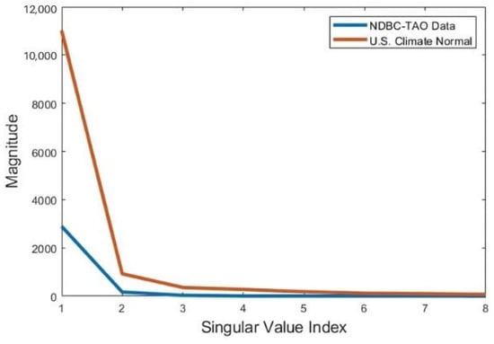
Figure 7. Low-rank structure within sensing data utilizing the singular values of the core tensor’s block diagonal matrices.

In Figure 7, it can be seen that each singular value has a different importance value, and the larger singular values contain more main data information; therefore, it is necessary to shrink different singular values using different weights rather than a fixed weight.

5.3. Experiment Setup

This section outlines a series of experiments conducted to confirm the efficacy of WRTPCA_WTNN, the proposed method. Its performance was compared with that of three other methods: the TRPCA [22], WTC [24], and the TRPCA combined with TC using the weighted sum tensor nuclear norm (TRPCA_TNN) [11]. This study used two real-world IoT datasets, namely the U.S. Climate Normal and NDBC-TAO datasets, to analyze their recovery under various conditions, including sparse mixed noise, outliers, and missing values. Various methods were used in these experiments to achieve optimal visual results.

All methods were carefully fine-tuned and tested repeatedly, 20 times in total, for all corrupted cases. The average values were calculated to obtain the results. Data corruption was characterized using four factors: Gaussian noise, impulsive noise, outliers, and missing values.

In extensive experiments, we assessed the performance of our model using different types of corrupted data. For Gaussian noise, we chose a zero mean and investigated ten variance levels (${\sigma }^2$) ranging from 11 to 20 in increments of one. Impulsive noise was examined at ten percentage levels (${\rho }_n$) from 0.1 to 0.55, with a step size of 0.05. Outliers were studied at ten magnitudes (k) ranging from 6 to 15 with a step size of 1, each being k times the standard deviation ($\sigma$) of each attribute. Missing values were explored at ten ratio levels (${\rho }_m$) from 0.1 to 0.55, with a step size of 0.05. Table 4 presents detailed parameters of the four corruption types.

Table 4. Detail parameters of each corruption type.

Corruption Type	Parameter	Range	Step Size
Gaussian noise	${\sigma }^2$	11 to 20	1
Impulsive noise	${\rho }_n$	0.1 to 0.55	0.05
Outlier	k	6 to 15	1
Missing value	${\rho }_m$	0.1 to 0.55	0.05

In each experimental case, we varied only the type of corruption across the levels and held the other parameters constant. The fixed values for the experiment were a Gaussian noise variance (${\sigma }^2$) set at 15, an impulsive noise percentage (${\rho }_n$) set at 0.3, an outlier magnitude (k) set at 15, and a missing ratio (${\rho }_m$) set at 0.3. For instance, in the Gaussian noise experiment, we altered the Gaussian noise variances (${\sigma }^2$) from 11 to 20 in steps of 1 while maintaining an impulsive noise percentage (${\rho }_n$) of 0.3, an outlier magnitude (k) of 15, and a missing ratio (${\rho }_m$) of 0.3.

Two algorithms, labeled Algorithms 3 and 4, were initialized with different WTSVT weight values. Specifically, $\omega =(1;1.9;2.1)$ was used in Algorithm 4, whereas $\omega =(1;1;1.6)$ was used in Algorithm 3. It was necessary to select appropriate values for ${\mu }_0$, ${\mu }_{max}$, $ϵ$, and $\rho$, which were the characteristics of the sensing data. In this study, the values of ${\mu }_0$, ${\mu }_{max}$, $ϵ$, and $\rho$ were set to $1\times {10}^{-1}$, $1\times {10}^{10}$, $1\times {10}^{-8}$, and $1.1$, respectively. The experimental results showed promising outcomes.

The experimental results were averaged across 20 replicates. All simulations used MATLAB R2021a on an Intel(R) Core(TM) i7-10700K CPU 3.80 GHz (Intel, Santa Clara, CA, USA).

5.4. Metrics

Reconstruction accuracy was evaluated using the normalized mean absolute error (NMAE). The NMAE for each of the three features considered in the dataset was determined by comparing the lateral slices of the input data with the reconstructed low-rank tensor.

$$NMAE=\frac{{\sum }_i^{n_2}\left|\mathcal{L}(:,i,:)-\widehat{\mathcal{L}}(:,i,:)\right|}{{\sum }_i^{n_2}\left|\mathcal{L}(:,i,:)\right|}$$

(24)

The original tensor is represented by $\mathcal{L}$, and the reconstructed low-rank tensor is denoted by $\widehat{\mathcal{L}}$. A comparison between the two tensors served as the foundation for the obtained results.

5.5. Results and Analysis

Each subfigure represents the results of the experiments, each involving a specific type of data corruption for a particular attribute within the datasets. The horizontal axis shows the levels of data corruption types, and the vertical axis illustrates the NMAE values of the four models in each case.

For Gaussian and impulsive noise, Figure 8 and Figure 9 illustrate the results of the comparison of our models and others on the NDBC-TAO and U.S. Climate Normal datasets. Across all models, the proposed model consistently outperformed the other methods. In particular, the NMAE values of our method applied to the two datasets consistently fell below 0.1 in most noise cases.

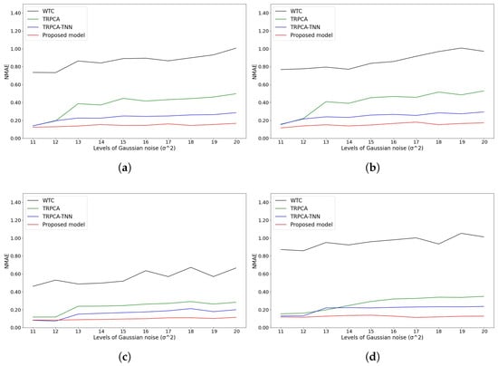
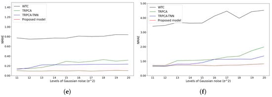
Figure 8. Reconstruction of Gaussian noise cases. (a) Temperature attribute of NDBC-TAO dataset; (b) density attribute of NDBC-TAO dataset; (c) salinity attribute of NDBC-TAO dataset; (d) dew attribute of U.S. Climate Normal dataset; (e) temperature attribute of U.S. Climate Normal dataset; (f) wind attribute of U.S. Climate Normal dataset.

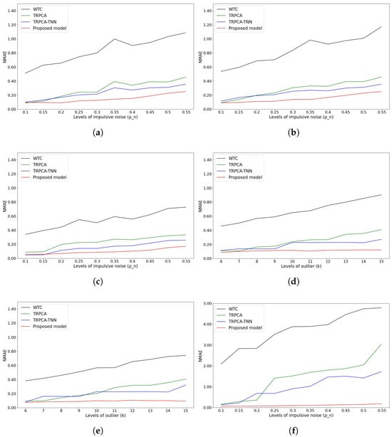
Figure 9. Reconstruction of impulsive noise cases. (a) Temperature attribute of NDBC-TAO dataset; (b) density attribute of NDBC-TAO dataset; (c) salinity attribute of NDBC-TAO dataset; (d) dew attribute of U.S. Climate Normal dataset; (e) temperature attribute of U.S. Climate Normal dataset; (f) wind attribute of U.S. Climate Normal dataset.

In addition, the proposed model can handle outliers. The NMAE values of all models in outlier cases are shown in Figure 10 for the two datasets. The results of the other models are worse than those of the proposed model, and the results of our model applied to the two datasets are below 0.1 in most outlier cases.

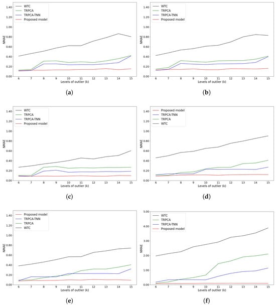
Figure 10. Reconstruction of outlier cases. (a) Temperature attribute of NDBC-TAO dataset; (b) density attribute of NDBC-TAO dataset; (c) salinity attribute of NDBC-TAO dataset; (d) dew attribute of U.S. Climate Normal dataset; (e) temperature attribute of U.S. Climate Normal dataset; (f) wind attribute of U.S. Climate Normal dataset.

Finally, the missing values are also reconstructed by our model, and the results of an experiment on the two datasets in the missing-value cases of the proposed model and the three different models are depicted in Figure 11. The experiment shows that the NMAE of the proposed model surpasses the NMAE values of the WTC, TRPCA, and TRPCA-TNN methods and maintains a value below 0.1 when applied to the two datasets in most missing-value cases.

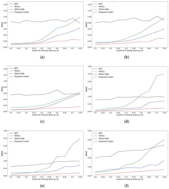
Figure 11. Reconstruction of missing value cases. (a) Temperature attribute of NDBC-TAO dataset; (b) density attribute of NDBC-TAO dataset; (c) salinity attribute of NDBC-TAO dataset; (d) dew attribute of U.S. Climate Normal dataset; (e) temperature attribute of U.S. Climate Normal dataset; (f) wind attribute of U.S. Climate Normal dataset.

Although each figure shows a comparison of the methods for each type of corruption, the default datasets consistently include a blend of noise, outliers, and missing values. Therefore, the reason the best outcomes were achieved by the proposed model is that it considers all types of corruption by employing WTSVT as a weighted approach for the TRPCA and TC, which shrinks singular values based on their significance and improves the capacity to reduce mixture noise and outliers and reconstruct missing values. Every singular value has distinct importance, as indicated in Section 5.2, and the more significant the data expressed, the greater the singular value. Therefore, we must reduce the distinct singular values using varying weights rather than fixed weights, as in most studies. In contrast, the WTC method consistently underperforms in all corruption cases. The WTC method performs poorly in all cases because it specializes in reconstructing missing values and performs poorly in reducing noise and outliers. The TRPCA method consistently outperforms the WTC method. However, it still requires consideration of the weights of the singular values to enhance its ability to handle mixed noise and outliers. In some cases with high missing value ratios, such as a missing value ratios from 0.4 to 0.55 in the dew attribute of the U.S Climate Normal dataset, the TRPCA performs worse than WTC. The effectiveness of the TRPCA in recovering missing values diminishes at higher missing value ratios because it is specifically designed to address noise and outlier problems, not missing data. The TRPCA is still helpful for some small ratios of missing values because the process extracts low-rank tensors that can recover but perform poorly. In addition, the TRPCA-TNN method performed better than the WTC and TRPCA methods but worse than the proposed model. This method combines the TRPCA, which specializes in noise and outliers, and TC solved using the weighted sum tensor nuclear norm, which specializes in missing values. The TRPCA in the TRPCA-TNN method does not consider the weights of singular values; therefore, the ability to reduce noise and outliers of the TRPCA-TNN method is still inferior to that of the proposed model. This model is still superior to the TRPCA at reducing noise and outliers because, in addition to the TRPCA, it also has a TC process that recovers missing values, which reduces noise and outliers with low accuracy. In the specialized recovery of missing values inthe TRPCA-TNN method, TC using the weighted sum tensor nuclear norm performs worse than TC using the weighted tensor nuclear norm. Owing to these limitations, the TRPCA-TNN method performed worse than the proposed model.

The performance of the U.S. Climate Normal dataset was lower than that of the NDBC-TAO dataset because the attributes in this dataset might have a low correlation as there are many attributes, such as temperature, wind statistics, mean sea level pressure, dew point, and cloud cover. However, we chose only three features, a number equal to the number of features in the NDBC-TAO dataset, to create the experimental dataset. In the NDBC-TAO dataset, the results for all scenarios of all models were consistently under 1.0 NMAE. Meanwhile, in the U.S. Climate Normal dataset, the results of other models in some complicated cases reached an NMAE of 5.0.

6. Conclusions

This study proposes a new technique for recovering multivariable data from 5G-based IoTs by combining TRPCA and TC approaches. The proposed approach can recover missing values, multiple noises, and outlier issues. By using the correlation between multi-attributes and solving problems using tensor data, this method can improve system performance. This uniqueness arises from the incorporation of WTSVT into TC and the TRPCA to handle singular values, which increases reconstruction accuracy by retrieving essential components. This combination overcomes the limitations of other models, such as WTC, the TRPCA, and the TRPCA-TNN, and significantly improves the ability to reduce mixed noise and outliers and reconstruct missing values. The proposed method is highly resistant to data corruption, including mixed noise, outliers, and missing values. Its NMAE consistently outperformed other metrics across two datasets, the NDBC-TAO and U.S. Climate Normal datasets. This method can be useful in various applications, particularly those related to the 5G-based IoT in real-world scenarios. Thus, these findings bridge the gap in the literature regarding better ways to handle extensive data analysis within the IoT environment.

Our objective in the near future is to automate the process of choosing the most appropriate weight for a particular dataset. This will allow us to utilize the most efficient and precise decision-making methods. Furthermore, we will explore situations in which there is a correlation between errors or noise, such as when one type of error is dependent on another. In addition, we will consider ways to reduce the complexity of the proposed algorithm.

References

- Elsheakh, D.; Shawkey, H. 5G wideband on-chip dipole antenna for WSN soil moisture monitoring. Int. J. RF Microw. Comput.-Aided Eng. 2021, 31, e22556. [Google Scholar] [CrossRef]
- Shawkey, H.; Elsheakh, D. Multiband dual-meander line antenna for body-centric networks’ biomedical applications by using UMC 180 nm. Electronics 2020, 9, 1350. [Google Scholar] [CrossRef]
- Alliance, N. 5G white paper. In Next Generation Mobile Networks, White Paper; 2015; Volume 1, Available online: https://pub.deadnet.se/Books%20and%20Docs%20on%20Hacking/Networking/Wireless%20LAN/NGMN%205G%20White%20Paper%20V1.0.pdf (accessed on 12 May 2024).
- Jaladi, A.R.; Khithani, K.; Pawar, P.; Malvi, K.; Sahoo, G. Environmental monitoring using wireless sensor networks (WSN) based on IOT. Int. Res. J. Eng. Technol. 2017, 4, 1371–1378. [Google Scholar]
- Corke, P.; Wark, T.; Jurdak, R.; Hu, W.; Valencia, P.; Moore, D. Environmental wireless sensor networks. Proc. IEEE 2010, 98, 1903–1917. [Google Scholar] [CrossRef]
- Alippi, C.; Camplani, R.; Galperti, C.; Roveri, M. A robust, adaptive, solar-powered WSN framework for aquatic environmental monitoring. IEEE Sens. J. 2010, 11, 45–55. [Google Scholar] [CrossRef]
- Ko, J.; Lu, C.; Srivastava, M.B.; Stankovic, J.A.; Terzis, A.; Welsh, M. Wireless sensor networks for healthcare. Proc. IEEE 2010, 98, 1947–1960. [Google Scholar] [CrossRef]
- Sharma, N.; Kaushik, I.; Bhushan, B.; Gautam, S.; Khamparia, A. Applicability of WSN and biometric models in the field of healthcare. In Deep Learning Strategies for Security Enhancement in Wireless Sensor Networks; IGI Global: Hershey, PA, USA, 2020; pp. 304–329. [Google Scholar]
- Xie, K.; Ning, X.; Wang, X.; Xie, D.; Cao, J.; Xie, G.; Wen, J. Recover corrupted data in sensor networks: A matrix completion solution. IEEE Trans. Mob. Comput. 2016, 16, 1434–1448. [Google Scholar] [CrossRef]
- Majumder, B.D.; Roy, J.K.; Padhee, S. Recent advances in multifunctional sensing technology on a perspective of multi-sensor system: A review. IEEE Sens. J. 2018, 19, 1204–1214. [Google Scholar] [CrossRef]
- Rajesh, G.; Chaturvedi, A. Data reconstruction in heterogeneous environmental wireless sensor networks using robust tensor principal component analysis. IEEE Trans. Signal Inf. Process. Netw. 2021, 7, 539–550. [Google Scholar] [CrossRef]
- Zhang, X.; He, J.; Li, Y.; Chi, Y.; Zhou, Y. Recovery of corrupted data in wireless sensor networks using tensor robust principal component analysis. IEEE Commun. Lett. 2021, 25, 3389–3393. [Google Scholar] [CrossRef]
- He, J.; Li, Y.; Zhang, X.; Li, J. Missing and Corrupted Data Recovery in Wireless Sensor Networks Based on Weighted Robust Principal Component Analysis. Sensors 2022, 22, 1992. [Google Scholar] [CrossRef] [PubMed]
- Xiao, F.; Liu, W.; Li, Z.; Chen, L.; Wang, R. Noise-tolerant wireless sensor networks localization via multinorms regularized matrix completion. IEEE Trans. Veh. Technol. 2017, 67, 2409–2419. [Google Scholar] [CrossRef]
- Madi, G.; Sacuto, F.; Vrigneau, B.; Agba, B.L.; Pousset, Y.; Vauzelle, R.; Gagnon, F. Impacts of impulsive noise from partial discharges on wireless systems performance: Application to MIMO precoders. EURASIP J. Wirel. Commun. Netw. 2011, 2011, 186. [Google Scholar] [CrossRef]
- Al Samara, M.; Bennis, I.; Abouaissa, A.; Lorenz, P. An efficient outlier detection and classification clustering-based approach for WSN. In Proceedings of the 2021 IEEE Global Communications Conference (GLOBECOM), Madrid, Spain, 7–11 December 2021; pp. 1–6. [Google Scholar]
- Deng, Y.; Han, C.; Guo, J.; Sun, L. Temporal and spatial nearest neighbor values based missing data imputation in wireless sensor networks. Sensors 2021, 21, 1782. [Google Scholar] [CrossRef] [PubMed]
- Cheng, J.; Ye, Q.; Jiang, H.; Wang, D.; Wang, C. STCDG: An efficient data gathering algorithm based on matrix completion for wireless sensor networks. IEEE Trans. Wirel. Commun. 2012, 12, 850–861. [Google Scholar] [CrossRef]
- Magán-Carrión, R.; Camacho, J.; García-Teodoro, P. Multivariate statistical approach for anomaly detection and lost data recovery in wireless sensor networks. Int. J. Distrib. Sens. Netw. 2015, 11, 672124. [Google Scholar] [CrossRef]
- Srindhuna, M.; Baburaj, M. Estimation of missing data in remote sensing images using t-SVD based tensor completion. In Proceedings of the 2020 International Conference for Emerging Technology (INCET), Belgaum, India, 5–7 June 2020; pp. 1–5. [Google Scholar]
- Kilmer, M.E.; Martin, C.D. Factorization strategies for third-order tensors. Linear Algebra Its Appl. 2011, 435, 641–658. [Google Scholar] [CrossRef]
- He, J.; Zhou, Y.; Sun, G.; Geng, T. Multi-attribute data recovery in wireless sensor networks with joint sparsity and low-rank constraints based on tensor completion. IEEE Access 2019, 7, 135220–135230. [Google Scholar] [CrossRef]
- Li, T.; Ma, J. T-SVD based non-convex tensor completion and robust principal component analysis. In Proceedings of the 2020 25th International Conference on Pattern Recognition (ICPR), Milan, Italy, 10–15 January 2021; pp. 6980–6987. [Google Scholar]
- Mu, Y.; Wang, P.; Lu, L.; Zhang, X.; Qi, L. Weighted tensor nuclear norm minimization for tensor completion using tensor-SVD. Pattern Recognit. Lett. 2020, 130, 4–11. [Google Scholar] [CrossRef]
- Ng, M.K.P.; Yuan, Q.; Yan, L.; Sun, J. An adaptive weighted tensor completion method for the recovery of remote sensing images with missing data. IEEE Trans. Geosci. Remote Sens. 2017, 55, 3367–3381. [Google Scholar] [CrossRef]
- Cheng, Q.; Yuan, Q.; Ng, M.K.P.; Shen, H.; Zhang, L. Missing data reconstruction for remote sensing images with weighted low-rank tensor model. IEEE Access 2019, 7, 142339–142352. [Google Scholar] [CrossRef]
- Geng, J.; Wang, L.; Xu, Y.; Wang, X. A weighted nuclear norm method for tensor completion. Int. J. Signal Process. Image Process. Pattern Recognit. 2014, 7, 1–12. [Google Scholar] [CrossRef][Green Version]
- Candès, E.J.; Li, X.; Ma, Y.; Wright, J. Robust principal component analysis? J. ACM (JACM) 2011, 58, 1–37. [Google Scholar] [CrossRef]
- Kang, J.; Wang, Y.; Schmitt, M.; Zhu, X.X. Object-based multipass InSAR via robust low-rank tensor decomposition. IEEE Trans. Geosci. Remote Sens. 2018, 56, 3062–3077. [Google Scholar] [CrossRef]
- Zhang, A.; Liu, F.; Du, R. Probability-weighted tensor robust PCA with CP decomposition for hyperspectral image restoration. Signal Process. 2023, 209, 109051. [Google Scholar] [CrossRef]
- Ruhan, A.; Mu, X.; He, J. Enhance tensor RPCA-based Mahalanobis distance method for hyperspectral anomaly detection. IEEE Geosci. Remote Sens. Lett. 2022, 19, 6008305. [Google Scholar]
- Guyon, C.; Bouwmans, T.; Zahzah, E.H. Robust principal component analysis for background subtraction: Systematic evaluation and comparative analysis. Princ. Compon. Anal. 2012, 10, 223–238. [Google Scholar]
- Gao, Q.; Zhang, P.; Xia, W.; Xie, D.; Gao, X.; Tao, D. Enhanced tensor RPCA and its application. IEEE Trans. Pattern Anal. Mach. Intell. 2020, 43, 2133–2140. [Google Scholar] [CrossRef] [PubMed]
- Zhang, L.; Tan, T.; Gong, Y.; Yang, W. Fingerprint database reconstruction based on robust PCA for indoor localization. Sensors 2019, 19, 2537. [Google Scholar] [CrossRef]
- Liu, X.; Chen, X.; Li, J.; Chen, Y. Nonlocal weighted robust principal component analysis for seismic noise attenuation. IEEE Trans. Geosci. Remote Sens. 2020, 59, 1745–1756. [Google Scholar] [CrossRef]
- Chang, Y.; Yan, L.; Zhao, X.L.; Fang, H.; Zhang, Z.; Zhong, S. Weighted low-rank tensor recovery for hyperspectral image restoration. IEEE Trans. Cybern. 2020, 50, 4558–4572. [Google Scholar] [CrossRef]
- Mu, X.; He, J.; Zhang, J. Enhance tensor RPCA-LRX anomaly detection algorithm for hyperspectral image. Geocarto Int. 2022, 37, 11976–11997. [Google Scholar]
- Chander, B.; Kumaravelan, G. Outlier detection strategies for WSNs: A survey. J. King Saud Univ.-Comput. Inf. Sci. 2022, 34, 5684–5707. [Google Scholar] [CrossRef]
- Tay, D.B. Sensor network data denoising via recursive graph median filters. Signal Process. 2021, 189, 108302. [Google Scholar] [CrossRef]
- Wilson, A.M.; Panigrahi, T.; Dubey, A. Robust distributed Lorentzian adaptive filter with diffusion strategy in impulsive noise environment. Digit. Signal Process. 2020, 96, 102589. [Google Scholar] [CrossRef]
- Kilmer, M.E.; Braman, K.; Hao, N.; Hoover, R.C. Third-order tensors as operators on matrices: A theoretical and computational framework with applications in imaging. SIAM J. Matrix Anal. Appl. 2013, 34, 148–172. [Google Scholar] [CrossRef]
- Zhang, Z.; Ely, G.; Aeron, S.; Hao, N.; Kilmer, M. Novel methods for multilinear data completion and de-noising based on tensor-SVD. In Proceedings of the IEEE Conference on Computer Vision and Pattern Recognition, Columbus, OH, USA, 23–28 June 2014; pp. 3842–3849. [Google Scholar]
- Gu, S.; Xie, Q.; Meng, D.; Zuo, W.; Feng, X.; Zhang, L. Weighted nuclear norm minimization and its applications to low level vision. Int. J. Comput. Vis. 2017, 121, 183–208. [Google Scholar] [CrossRef]
- Gao, Q.; Xia, W.; Wan, Z.; Xie, D.; Zhang, P. Tensor-SVD based graph learning for multi-view subspace clustering. In Proceedings of the AAAI Conference on Artificial Intelligence, New York, NY, USA, 7–12 February 2020; Volume 34, pp. 3930–3937. [Google Scholar]
- Candes, E.J.; Plan, Y. Matrix completion with noise. Proc. IEEE 2010, 98, 925–936. [Google Scholar] [CrossRef]
- Gu, S.; Zhang, L.; Zuo, W.; Feng, X. Weighted nuclear norm minimization with application to image denoising. In Proceedings of the IEEE Conference on Computer Vision and Pattern Recognition, Columbus, OH, USA, 23–28 June 2014; pp. 2862–2869. [Google Scholar]
Disclaimer/Publisher’s Note: The statements, opinions and data contained in all publications are solely those of the individual author(s) and contributor(s) and not of MDPI and/or the editor(s). MDPI and/or the editor(s) disclaim responsibility for any injury to people or property resulting from any ideas, methods, instructions or products referred to in the content. |
© 2024 by the authors. Licensee MDPI, Basel, Switzerland. This article is an open access article distributed under the terms and conditions of the Creative Commons Attribution (CC BY) license (https://creativecommons.org/licenses/by/4.0/).