Article

Frequency-Separated Attention Network for Image Super-Resolution

1
School of Information and Control Engineering, China University of Mining and Technology, Xuzhou 221116, China
2
School of Energy and Materials Engineering, Shandong Polytechnic College, Jining 272067, China
3
School of Computer Science and Technology, China University of Mining and Technology, Xuzhou 221116, China
*
Author to whom correspondence should be addressed.
Appl. Sci. 2024, 14(10), 4238; https://doi.org/10.3390/app14104238
Submission received: 28 March 2024 / Revised: 9 May 2024 / Accepted: 15 May 2024 / Published: 16 May 2024
(This article belongs to the Special Issue Advanced Pattern Recognition & Computer Vision)

Abstract

:
The use of deep convolutional neural networks has significantly improved the performance of super-resolution. Employing deeper networks to enhance the non-linear mapping capability from low-resolution (LR) to high-resolution (HR) images has inadvertently weakened the information flow and disrupted long-term memory. Moreover, overly deep networks are challenging to train, thus failing to exhibit the expressive capability commensurate with their depth. High-frequency and low-frequency features in images play different roles in image super-resolution. Networks based on CNNs, which should focus more on high-frequency features, treat these two types of features equally. This results in redundant computations when processing low-frequency features and causes complex and detailed parts of the reconstructed images to appear as smooth as the background. To maintain long-term memory and focus more on the restoration of image details in networks with strong representational capabilities, we propose the Frequency-Separated Attention Network (FSANet), where dense connections ensure the full utilization of multi-level features. In the Feature Extraction Module (FEM), the use of the Res ASPP Module expands the network’s receptive field without increasing its depth. To differentiate between high-frequency and low-frequency features within the network, we introduce the Feature-Separated Attention Block (FSAB). Furthermore, to enhance the quality of the restored images using heuristic features, we incorporate attention mechanisms into the Low-Frequency Attention Block (LFAB) and the High-Frequency Attention Block (HFAB) for processing low-frequency and high-frequency features, respectively. The proposed network outperforms the current state-of-the-art methods in tests on benchmark datasets.

1. Introduction

Image super-resolution is an ill-posed problem that transforms a given coarse, low-resolution (LR) image into a high-resolution (HR) image with refined details. Traditional super-resolution methods include interpolation, sparse coding [1], and neighbor embedding [2]. However, these methods do not effectively map LR images to HR images.
Recently, convolutional neural networks (CNNs) have demonstrated superior expressive capabilities compared to traditional methods, achieving outstanding performance and efficiency in various high-level imaging tasks. SRCNN [3] first upscales an LR image to the size of an HR image using bicubic interpolation and then applies a convolutional neural network to replace the traditional manual mapping from LR to HR images, surpassing most traditional methods. CSCN [4] and SCN [5] enhance network expressiveness by integrating the traditional super-resolution (SR) method and a sparse prior with key components of neural convolutional networks. The deeper the network, the stronger its non-linear mapping capability; however, this depth can also result in weakened information flow and training difficulties. VDSR [6] focuses on residual learning of the differences between HR and LR images, further increasing the network depth. Additionally, the introduction of recursive modules [7,8] and memory modules [7] also enhances depth. FSRCNN [9] increases network depth by reducing the size of filters. FSRCNN [9] and ESPCN [10] introduced deconvolution and sub-pixel convolution layers, respectively, a structure later adopted by most networks. Tai et al. [11] and Lim et al. [12] further increased network depth using residual blocks, while Tong et al. [13] and Zhang et al. [14,15] introduced data particle geometrical divide algorithms to the field of super-resolution. The authors of [16] added numerous skip connections to mitigate information flow attenuation in overly deep networks. To enhance the network’s ability to process high-frequency information, Zhao et al. [17] employed deep convolutional networks and ResNet for high-frequency information in images, while Zhou et al. [18] identified high-frequency features and increased their learning rates to improve the recovery of complex details in images.
Due to the optimal loss function for super-resolution problems being L 1 , resulting in minimal loss values, the combination of small loss values and excessive layers in deep networks can lead to gradient vanishing. Consequently, it becomes challenging to effectively translate the potential expressive capabilities gained from increased network depth into the model’s ability to learn the non-linear mapping from LR to HR images. Images contain high-frequency information representing texture details and low-frequency information describing object edges; similarly, features extracted by the network from LR images also consist of low- and high-frequency features. The use of numerous skip connections for dense connectivity allows for the full, adaptive integration of features across layers, and the use of memory modules achieves persistent memory, mitigating the effects of information flow attenuation caused by network depth. High-frequency features require more complex processing for detailed restoration compared to low-frequency features. However, the absence of an effective network structure to distinguish between high- and low-frequency information in images results in outputs where parts with complex textures appear smooth. Zhao et al. [17] and Zhou et al. [18] processed high- and low-frequency features separately, but in deep convolutional networks, some informative features may be overlooked.
To address these issues, we propose a Frequency-Separated Attention Network, termed FSANet, for image super-resolution. FSANet employs dense connections to fully integrate multi-level features for sustained memory, separately processes high- and low-frequency features to meet the demands of high-frequency feature processing, and utilizes channel and spatial attention to leverage informative features in both high- and low-frequency domains. In FSANet, we design an FEM for feature extraction and a Non-Linear Mapping Module (NMM) for the non-linear mapping of features from LR to HR. The FEM contains a convolutional layer and two Res ASPP Modules, expanding images into a high-dimensional feature space and increasing the receptive field, respectively. In the NMM, three FSABs are stacked, and the results of these FSABs are adaptively fused to fully leverage global multi-level features. Each FSAB employs an LF path for low-frequency features and an HF path for high-frequency features, with the LF path containing three densely connected Low-Frequency Attention Modules (LFAMs) and the HF path containing three densely connected High-Frequency Attention Modules (HFAMs). Within the HFAM, an HFAB and a Fusion Block are integrated, with the HFAB incorporating a projection error mechanism for processing high-frequency features. Similarly, the LFAM includes an LFAB and a Fusion Block for processing low-frequency features. To fully utilize informative features and enhance the details in image restoration, we introduce attention mechanisms in both the LFAB and HFAB.
In summary, the main contributions of the proposed image SR method are as follows:
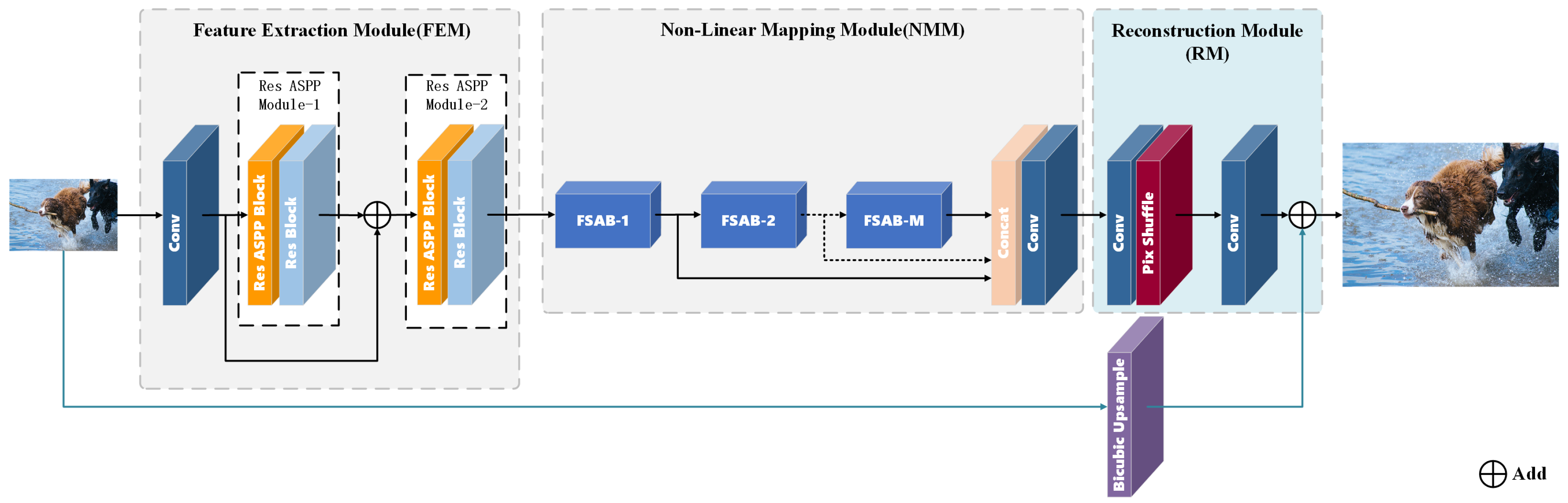
  • We introduce the novel deep convolutional neural network FSANet for image super-resolution tasks, utilizing a densely connected structure to leverage the powerful representational capability of deep CNNs and employing a parallel branching structure to separately process high- and low-frequency features.
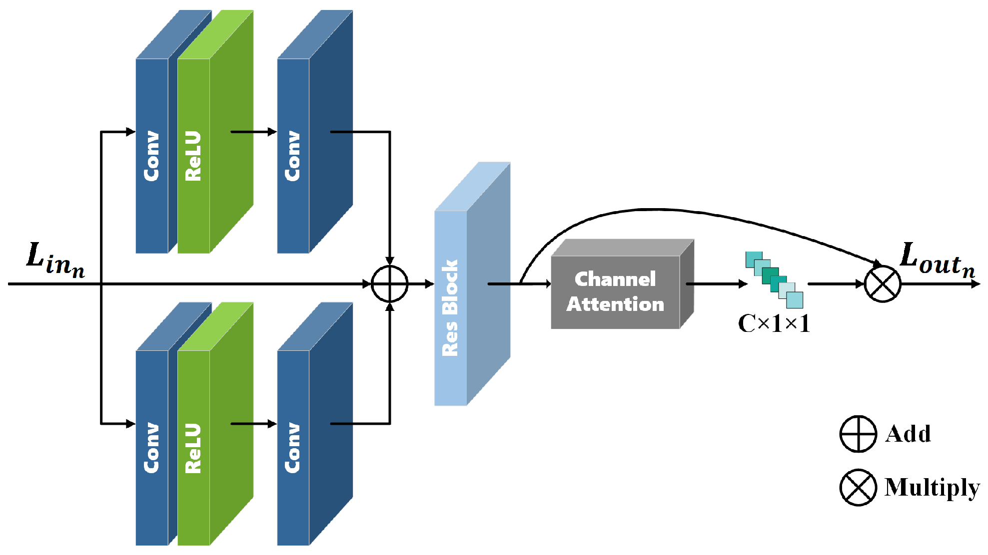
  • To further enhance the quality of the network’s output images, we incorporate attention mechanisms in the LFAB and HFAB to fully exploit informative features across both channel and spatial dimensions.
  • Experimental results demonstrate that our proposed method achieves higher performance compared to state-of-the-art super-resolution methods.

2. Related Work

There is a huge amount of work on image super-resolution, and thus, a comprehensive survey on SR methods is beyond the scope of this paper. This section provides a brief overview of some related works that are based on deep learning methods, frequency-separated networks, and attention networks.

2.1. Image Super-Resolution Based on Deep Learning

Compared to traditional mathematical methods, neural networks possess superior non-linear matching capabilities. SR methods based on deep learning include different usage scenarios, such as those based on classic blind image SR [3], non-blind image SR [19], real image SR [20], text-focused scene image SR [21], lightweight image SR [22], hyperspectral image SR [23], video SR [24], attenuation correction SR [25,26], etc. Dong et al. first introduced SRCNN [3], which contains three convolutional layers, to address super-resolution issues. To regularize the solution, CSCN [4] and SCN [5] integrate traditional sparse coding with deep learning, demonstrating the value of conventional methods in deep neural networks. Unlike networks that upscale LR images to an HR size before input, ESPCN [10] and FSRCNN [9] directly learn the mapping from LR to HR, effectively increasing the network’s responsiveness. At the end of the network, the sub-pixel convolution and deconvolution layers are used to obtain SR images. This network structure significantly influenced the design of subsequent SR networks.
Vgg-net [27] indicates that deeper networks can perform more complex non-linear mappings, thereby enhancing the restoration of details in SR images. Since normalization in super-resolution networks can lead to artifacts and slow and unstable training, SR networks employ alternative methods to address the vanishing gradient problem, facilitating easier network training. Since LR and HR images share most fundamental features, VDSR [6] employs the residual learning of the differences between LR and HR images, not only increasing the network layers to 20 but also enhancing the network’s convergence speed. MemNet [7] uses memory blocks containing recursive and gate units to address the issue of weakened information flow due to increased network depth. Unlike increasing the number of convolutional layers to deepen the network, DRCN [8] employs a very deep recursive layer to enhance the network’s feature abstraction and parameter sharing, while recursive supervision and skip connections are used to mitigate the effects of network depth. Residual blocks [28] are used in networks [11,12] to address the vanishing gradient problem, further increasing network depth and representational capacity. To further increase network depth, Tong et al. [13] and Zhang et al. [16] directly connected the current layer with all subsequent layers using dense skip connections. This forms a contiguous memory mechanism, adaptively integrating information from multiple levels. Deep learning-based methods have shown exceptional performance in super-resolution tasks. The proposed method is based on deep learning.

2.2. Frequency-Separated Networks

To enhance training speed and performance, Zhao et al. [17] utilized deep convolutional networks and ResNet for high-frequency information storage and expanded the network’s receptive field, increasing the accuracy of detail restoration in images. SRDN [18] employs a densely connected convolutional neural network for high-frequency information enhancement, increasing the learning rate for high-frequency areas to focus more on reconstructing high-frequency regions in images. SRFBN [29] consists of feedback blocks using a feedback mechanism, providing high-level information through a series of up- and downsampling layers. FSN [30] divides image features into high and low frequencies for respective processing, employing Octave Convolution to maintain a good interaction between low- and high-frequency information. DBPN [31] introduces iterative upsampling and downsampling layers, where the Up-Projection Unit generates high-frequency features, and the Down-Projection Unit produces low-frequency features. Yang et al. [32] proposed a deep recursive low-frequency fusion network and designed a variance-based channel attention mechanism to make the information distribution of each feature map under different variances more reasonable. Refs. [17,18] only processed high-frequency features in images, overlooking the significance and importance of low-frequency features. In contrast, our method extracts both low- and high-frequency information. While we also focus on processing high-frequency features similar to [17,18], we do not neglect the processing of low-frequency features. This approach ultimately enhances the performance of the network.

2.3. Attention Networks

The attention mechanism offers a new perspective for task resolution, learning crucial information from inputs and demonstrating superiority in various computer vision tasks, such as object detection, image segmentation, and action recognition. The authors who proposed SCA-CNN [33] argued that previous spatial attention models only considered information within the CNN’s spatial and multilayer contexts; hence, they introduced channel attention to discern which channels are most important for generating image captions. DANet [34] enhances context capture by adding positional and channel self-attention modules to model semantic relations in both the spatial and channel dimensions, resulting in finer scene segmentation outcomes. Zhang et al. [35] employed an attention mechanism for the selective integration of multi-level features, reducing background interference and enhancing object detection performance.
Liu et al. [36] used an attention mechanism to distinguish and enhance high-frequency information, improving detail restoration. LR images contain both low- and high-frequency information treated equally, thus diminishing detail restoration. Hence, RCAN [37] combines channel attention with residuals, allocating more computation to high-frequency information as network depth increases. Lu et al. [38] employed recursive units with channel attention to extract significant features from channels, using multi-level feature fusion techniques for feature enhancement. In CSFM [39], spatial and channel attention mechanisms, along with dense connections, are used to distinguish critical features across dimensions and mitigate the weakening of information flow in deep networks. The aforementioned works utilized attention mechanisms in super-resolution tasks but did not consider feature separation to alleviate the learning difficulty of attention mechanisms. By separating high- and low-frequency features in images and processing them differently, our approach enables attention mechanisms to focus on learning distinct features for backgrounds (low-frequency features) and complex texture features (high-frequency features) separately. This reduces the network’s learning burden while enhancing its ability to distinguish between these two types of features.

3. Method

In order to use a densely connected structure to leverage the powerful representational capability of deep CNNs and separate process high- and low-frequency features, in this paper, we propose a Frequency-Separated Attention Network for image super-resolution, termed FSANet. First, we introduce the overall network architecture in Section 3.1. Second, we present the frequency-separated attention block in Section 3.2. Third, we describe the High-Frequency Attention Module in Section 3.3. And last, we present the Low-Frequency Attention Module in Section 3.4.

3.1. Network Architecture

As shown in Figure 1, our proposed FSANet consists of the Feature Extraction Module (FEM), Non-Linear Mapping Module (NMM), and Reconstruction Module (RM). We use I L R , I S R , and I H R to denote the input, output, and high-resolution image of FSANet, respectively. In the FEM, I L R is first passed through a convolution layer for feature extraction. The output g c o n v is then processed by two Res ASPP Modules, each of which contains three parallel deep CNNs to expand the receptive field and obtain multi-scale features.
g K 2 = f F E M ( I L R ) = f K 2 ( f K 1 ( f c o n v ( I L R ) ) + f c o n v ( I L R ) ) = f K 2 ( g K 1 + g c o n v ) .
Here, f F E M ( · ) denotes the FEM, and f c o n v ( · ) represents the 3 × 3 convolution producing g c o n v . f K 1 ( · ) and f K 2 ( · ) denote two Res ASPP Modules with the outputs g K 1 and g K 2 , respectively.
In the NMM, three FSABs are linearly stacked. Assuming that the input of the m-th FSAB is F m 1 and its output is F m , then the input for the first FSAB is F 0 (i.e., g K 2 ), and the output of the last FSAB is F M . The m-th FSAB is as follows:
F m = f F S A B m f F S A B m 1 f F S A B 1 F 0 .
Here, f F S A B m ( · ) represents the m-th FSAB. Each FSAB outputs distinct features. To fully utilize these hierarchical features, we adopt an adaptive fusion of long-term multi-level features, concatenating the outputs of the three FSABs before feeding them into a convolution layer. Thus, the NMM is as follows:
g N M M = f N M M F 0 = φ c o n v ( [ F 1 , F 2 , , F M ] ) .
Here, f N M M ( · ) denotes the NMM, φ c o n v ( · ) represents the 3 × 3 convolution yielding g N M M , and [ · ] signifies the feature concatenation operation.
In the RM, we employ convolution and sub-pixel convolution layers [10] for upsampling to obtain I S R . Additionally, we utilize a global skip connection through bicubic upsampling to maintain long-term memory.
I S R = f R M g N M M + B i c u b i c I L R = f R M f N M M f F E M I L R + B i c u b i c I L R ,
where f R M ( · ) denotes the RM, and B i c u b i c ( · ) represents the bicubic upsampling operation.
According to [16], the Peak Signal-to-Noise Ratio (PSNR) is highly correlated with the pixel-wise differences between I S R and I H R . Given that the L 2 loss function tends to emphasize larger differences and weaken smaller ones, and considering that its convergence is inferior to that of the L 1 loss function, we use the L 1 loss function to optimize FSANet. Given a set of training patch pairs { I L R i , I H R i } i = 1 I , the loss function of FSANet is as follows:
L θ = 1 I i = 1 I F F S A N e t I L R i I H R i 1 ,
where F F S A N e t ( · ) denotes FSANet, and θ represents the parameters within FSANet.

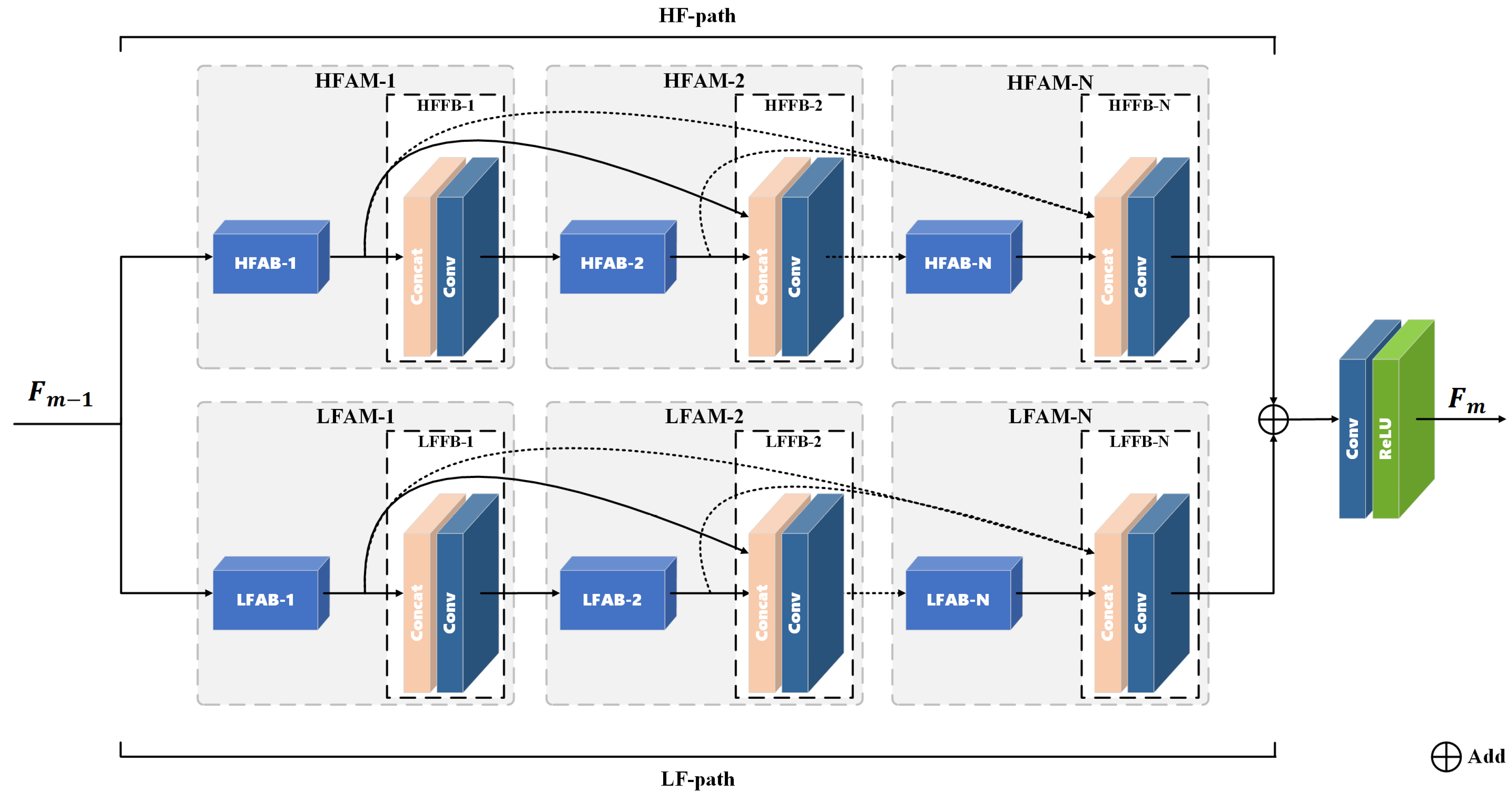
3.2. Frequency-Separated Attention Block

The extracted high-frequency features, compared to low-frequency features, contain more information and thus require more processing, for which we propose the FSAB. As shown in Figure 2, the m-th FSAB consists of two branches: a high-frequency path (HF path) formed by three HFAMs to process high-frequency features and a low-frequency path (LF path) formed by a linear stack of LFAMs to process low-frequency features.
H i n n represents the input to the n-th HFAB, while H o u t n represents the output. There are a total of N HFABs. The equation is given by
H o u t n = f H F A B n H i n n .
Here, f H F A B n ( · ) represents the n-th HFAB, which is detailed in Section 3.3. The expression for the n-th High-Frequency Fusion Block (HFFB) is as follows:
F H F F B n = f H F F B n H o u t 1 , , H o u t n ,
where f H F F B n ( · ) denotes the convolution in the n-th HFFB, with its output being F H F F B n .
In the LF path, let L i n n be the input and L o u t n be the output of the n-th LFAB:
L o u t n = f L F A B n L i n n .
f L F A B n ( · ) represents the n-th LFAB, which is emphasized in Section 3.4. To achieve relatively high performance, we use Low-Frequency Fusion Blocks (LFFBs) for multi-level dense local feature fusion by directly connecting the output of the current and previous LFABs to the LFFB. Consequently, the expression for the n-th LFFB is as follows:
F L F F B n = f L F F B n L o u t 1 , , L o u t n .
f L F F B n ( · ) represents the n-th LFFB, with its output denoted by F L F F B n .
Finally, the outputs of both branches are added to merge high-frequency and low-frequency information. The output of the FSAB is generated through a deep CNN to complement the advantages of high- and low-frequency features. The m-th FSAB is as follows:
F m = f F S A B m F m 1 = R e L U ϕ F L F F B N + F H F F B N = R e L U ϕ f L F F B N L o u t 1 , , L o u t N + f H F F B N H o u t 1 , , H o u t N ,
Here, ϕ ( · ) represents the convolution, and R e L U ( · ) indicates the ReLU layer.

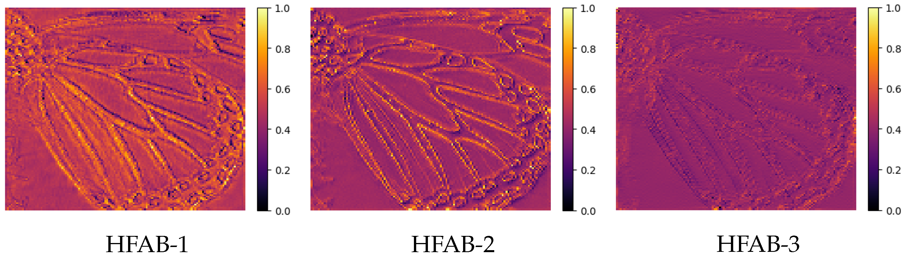
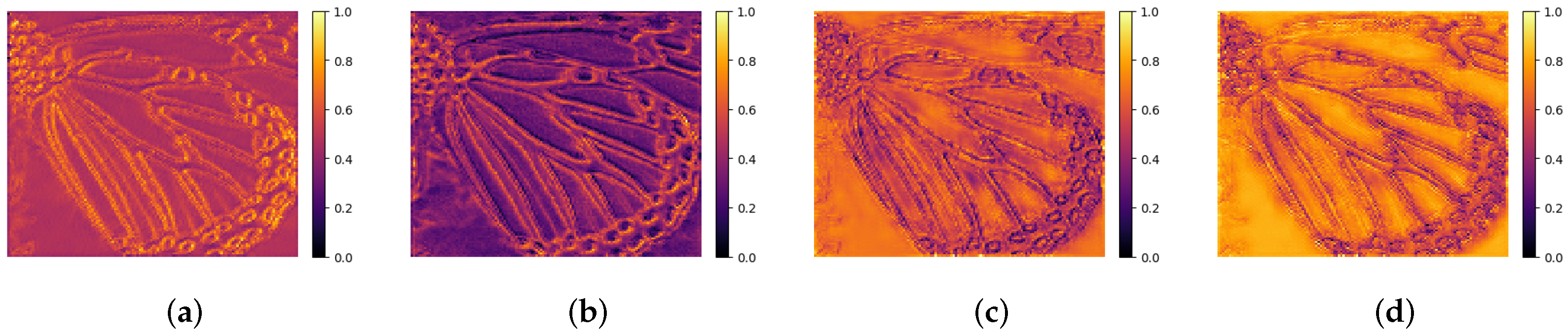
3.3. High-Frequency Attention Module

In this section, we introduce two parts (the architectures of the HFAB and the High-Frequency Block) of the High-Frequency Attention Module in detail.

3.3.1. The Architecture of the HFAB

As illustrated in Figure 3, the HFAB primarily comprises three components: a linear stack of High-Frequency Blocks (HFBs), a Frequency Fusion Block, and a CSA Module. Let the input of the t-th HFB be F H F B t 1 and the output be F H F B t . Thus, the t-th HFB can be defined as follows:
F H F B t = f H F B t f H F B t 1 f H F B 1 F H F B 0 ,
where f H F B t ( · ) represents the t-th HFB. In the experiment, t { 1 , 2 , 3 } .
As the network deepens, the features within each HFB layer differ. To fully utilize this information, we employ a Frequency Fusion Block for multi-level local feature fusion. The Frequency Fusion Block selectively fuses the outputs from the preceding HFB by utilizing a Concat layer and processing them through a deep CNN. The result F F r e F serves as the input for the CSA Module and is defined as follows:
F F r e F = f F r e F ( [ F H F B 1 , , F H F B T ] ) = R e L U ( ψ ( [ F H F B 1 , , F H F B T ] ) ) ,
where f F r e F ( · ) denotes the Frequency Fusion Block, and ψ ( · ) represents the convolution in the Frequency Fusion Block.
Distinct features play varied roles in image reconstruction. To enhance the network’s sensitivity to crucial features, we utilize a CSA Module [39] incorporating channel attention and spatial attention to selectively strengthen features in both the channel and spatial dimensions. Spatial attention, in particular, aids in distinguishing between smooth areas and texture features. Within the CSA Module, features modified by attention mechanisms are adaptively fused and then skip-connected with the original features, thus selectively enhancing features without losing information from the original ones. The n-th HFAB can be defined as follows:
H o u t n = f H F A B n H i n n f C S A M ( F F r e F ) = f A t t F f S A F F r e F F F r e F , f C A F F r e F F F r e F + F F r e F ,
where f C S A M ( · ) denotes the CSA Module, f S A ( · ) [39] and f C A ( · ) [39] represent spatial attention and channel attention, respectively, and f A t t F ( · ) is the convolution function within the Attention Fusion Block.

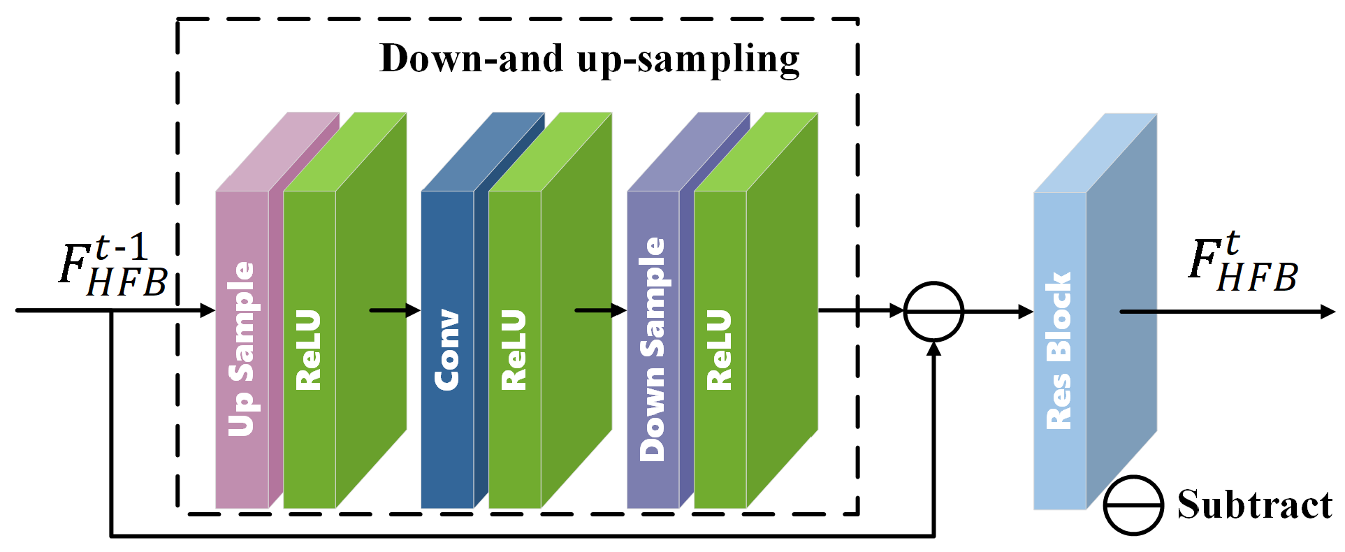
3.3.2. The Architecture of the HFB

In D-DBPN [31], an iterative error-correcting feedback mechanism was introduced, and Timoft et al. [40] demonstrated that high-frequency information can be progressively refined by continuously subtracting the results of upsampling and downsampling from the original input. To better process high-frequency features, a deep CNN is applied in the middle of down- and upsampling. To reduce the degradation of the original information after one iteration of refinement, a residual block is added. F H F B t 1 and F H F B t are defined as the input and output of the t-th HFB, respectively, with down- and upsampling specified as follows:
F p r o j e c t = f p r o j e c t F H F B t 1 = R e L U f d o w n R e L U f c o n v R E L U f u p F H F B t 1 .
F p r o j e c t and f p r o j e c t ( · ) represent the output and function of down- and upsampling [31], respectively. Here, f u p ( · ) is the function for deconvolution operations, and both f c o n v ( · ) and f d o w n ( · ) represent convolution operations. The HFB can be defined as follows:
F H F B t = f H F B F H F B t 1 = f r e s b l o c k f p r o j e c t F H F B t 1 F H F B t 1 .
Here, f r e s b l o c k ( · ) is the function for the residual block [28], as illustrated in Figure 4.

3.4. Low-Frequency Attention Module

We utilize the Low-Frequency Attention Block (LFAB) to process low-frequency features, employing a tri-branch structure for handling the low-frequency features L i n n , as illustrated in Figure 5. One branch retains the original input information, corresponding to the middle branch in Figure 5. Another branch utilizes a deep CNN and a convolutional layer with a kernel size of 3 × 3 , depicted as the top branch in Figure 5. The final branch comprises a deep CNN and a convolutional layer with a kernel size of 5 × 5 to expand the field of view, shown as the bottom branch in Figure 5. To mitigate the impact of increased network depth on feature attenuation and selective enhancement across different channels, we perform an additive operation on the three branches before passing the result through a residual block and a channel attention mechanism to obtain the output L o u t n of the t-th LFAB,
L o u t n = f L F A B n L i n n = f b r a n c h r e s ( L i n n ) f C A f b r a n c h r e s ( L i n n ) = F b r a n c h r e s f C A F b r a n c h r e s ,
where f b r a n c h r e s ( · ) denotes the tri-branch and a Res Block in Figure 5, and f C A ( · ) [39] represents channel attention.

4. Experiments

In this section, we first conduct an ablation study to validate the effectiveness of the proposed FSANet network architecture. Then, we compare FSANet with several other networks on benchmark datasets in terms of the PSNR and SSIM. We follow the approach of previous work [39] to train and test our model. We use the DIV2K [40] dataset, which contains 800 high-quality images, for training.

4.1. Settings

In this section, we present the datasets, metrics, and implementation details.

4.1.1. Datasets and Metrics

We train and test our network following methods in prior work [16]. LR images in DIV2K are obtained by bicubic downsampling of HR images by factors of ×2, ×3, and ×4. We evaluate our model on widely used benchmark datasets: Set5 [41], Set14 [42], BSD100 [43], Urban100 [44], and Manga109 [45], which contain 5, 14, 100, 100, and 109 images, respectively, covering common scenes from daily life. The model evaluation metrics include the Peak Signal-to-Noise Ratio (PSNR) and Structural Similarity Index Measure (SSIM) [46], with results computed on the Y channel (i.e., luminance) of the YCbCR space. Higher PSNR and SSIM values closer to 1 indicate better quality of the reconstructed SR images.

4.1.2. Implementation Details

During training, data augmentation is performed through random vertical and horizontal flips and 90° rotations around the image center, with a mini-batch size of 16 and the random cropping of 64 × 64 patches from LR images for input. Following the method in [39], the input to the model is normalized by subtracting the mean RGB values of DIV2K to highlight individual feature differences, and the mean RGB values of DIV2K are added back before the network output. We use the ADAM optimizer with an initial learning rate of 10 4 to train the network, halving the learning rate after 1.5 × 10 5 and 2 × 10 5 iterations. We implement FSANet using PyTorch and conduct training and testing on an NVIDIA RTX 3090 GPU.
The Res ASPP Block [47] includes three dilated convolutions with dilation rates of 1, 4, and 8. In RM, the first convolutional layer has filters of 256, 576, and 1024 for magnification factors of ×2, ×3, and ×4, respectively. The second layer has 3 filters. And all other layers have 64 filters each. The values of N and M are both set to 3. The reduction ratio in channel attention is 16, and the increase ratio in spatial attention is 2.

4.2. Ablation Study

In this section, we show the effectiveness of Res ASPP feature extraction, frequency-separated structures, and attention mechanisms.

4.2.1. The Effectiveness of Res ASPP Feature Extraction

We utilized the Res ASPP Module to enhance the field of view for improved feature extraction. To verify the effectiveness of the Res ASPP Module, we conducted the following experiments: (1) removing the Res ASPP Module from the FEM; (2) retaining the Res ASPP Module within the FEM. As shown in Figure 6, we visualized the average feature maps after feature extraction from both experiments. The outputs of feature extraction were as follows: for experiment (1), the result of the first convolution g c o n v in the Feature Extraction Module, and for experiment (2), the results of the first convolution g c o n v and the output of Res ASPP Module-2 g K 2 . From the feature maps, it is evident that the contours of the feature maps without the Res ASPP Module are discontinuous and blurred. This could be due to misinterpreting adjacent similar features as dissimilar or vice versa within a limited field of view. Based on the test results on the benchmark dataset outlined in Table 1, the outcomes without the Res ASPP Module consistently underperform compared to those with it, thereby validating the effectiveness of the Res ASPP Module. Moreover, as evident from Figure 7a, the utilization of the Res ASPP Module accelerates the convergence of the network during training by enhancing feature extraction.

4.2.2. The Effectiveness of Frequency-Separated Structures

The FSAB consists of an LF path (for low-frequency information) and an HF path (for high-frequency information).
In Figure 8 and Figure 9, we visualize the average feature maps of low- and high-frequency information from the first three FSABs. The low-frequency information feature maps depict the general contours, while the high-frequency information feature maps describe the edges and textures. To verify the effectiveness of separating high- and low-frequency structures, we conducted the following experiments: (1) the FSAB containing only the LF path, (2) the FSAB containing only the HF path, (3) the FSAB containing both the LF path and HF path. To roughly maintain equal parameters, the first two experiments used 13 and 4 FSABs, respectively.
Figure 7b displays the PSNR results of the three experiments tested on the Set5 dataset during the training process, and Table 2 shows the test results of the three experiments on standard datasets. We found that using both the LF path and HF path for image reconstruction yielded better results and faster convergence than using either path alone.

4.2.3. The Effectiveness of Attention Mechanisms

To verify the effectiveness of attention mechanisms, we removed all attention modules from the LF path and HF path in the original model and retrained it. As shown in Figure 10, we extracted the average feature maps from the LF path and HF path both with and without attention modules. The figures reveal that in the LF path, contours (low-frequency information) are highlighted in the feature maps. However, the use of attention causes the LF path to focus more on low-frequency information, making the texture areas (high-frequency information) with attention dimmer than those without. In the HF path, textures (high-frequency information) are highlighted, and the use of attention ensures that similar textures (high-frequency information) are processed similarly. As indicated in Table 3, we also conducted tests on standard datasets and found that the results with attention modules are better than those without.

4.3. Comparison with State-of-the-Art Methods

In this section, we show the visualization of PSNR and SSIM results and the analysis results of model comparisons.

4.3.1. Comparison and Visualization of PSNR and SSIM Results

In this section, we compare our FSANet with state-of-the-art methods, including SRCNN [3], FSRCNN [9], VDSR [6], HDRN [48], CARN [49], MemNet [7], IMDN [50], LAPAR-A [51], SRMD [52], A2F-L [53], and FENet [54].
Table 4 presents the values of the PSNR and SSIM metrics for different networks at magnification factors of ×2, ×3, and ×4 on five benchmark datasets commonly used in super-resolution. Figure 11 displays a visual quality comparison of image reconstructions at a magnification factor of 4×. The images reconstructed by FSANet exhibit more vivid details compared to those from other networks, as shown in the figures.

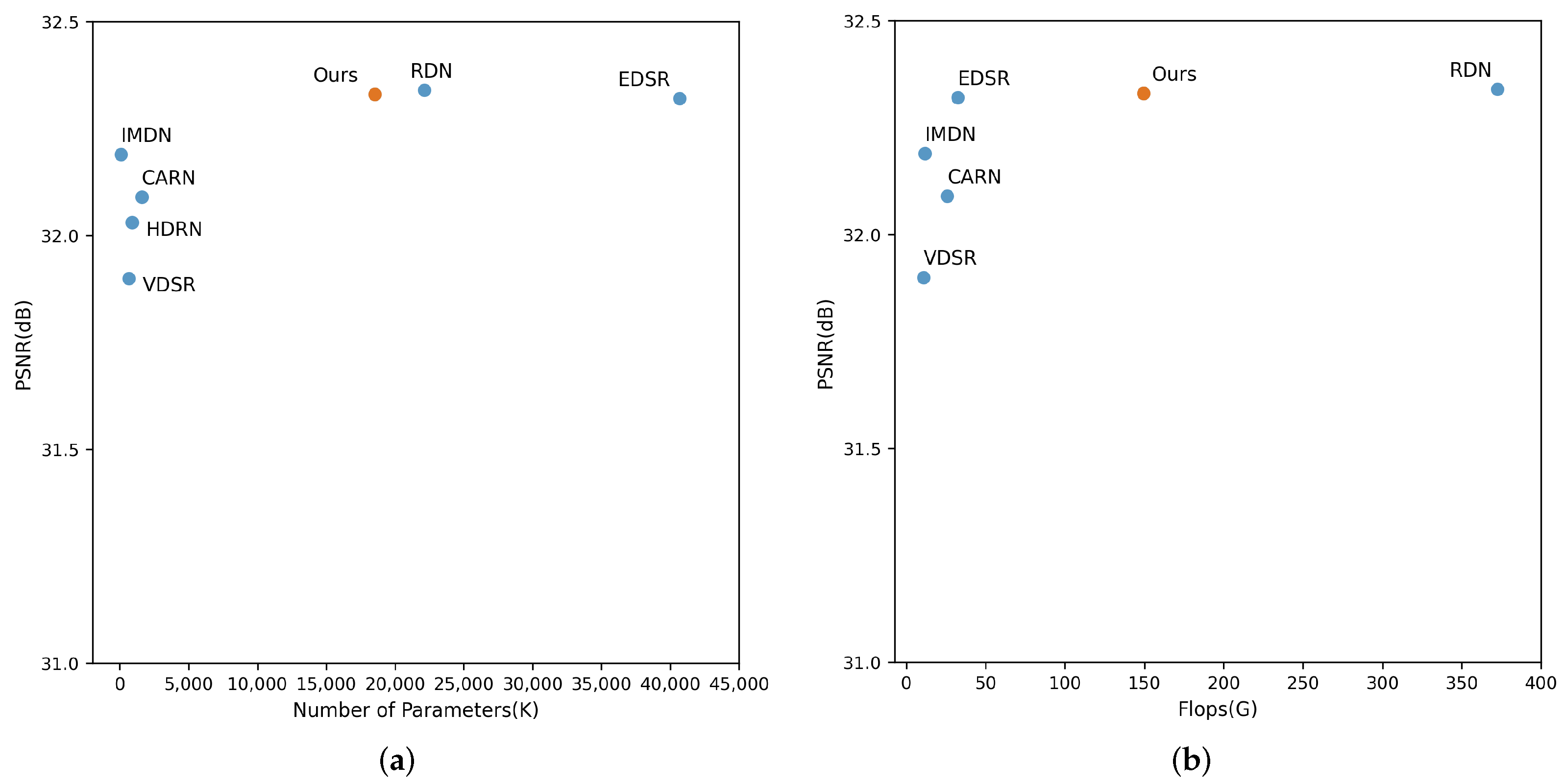
4.3.2. Analysis of Model Comparisons

As illustrated in Figure 12a, we compared the super-resolution performance and parameter count of our FSANet at a magnification factor of ×2 with existing models, namely, VDSR [6], HDRN [48], CARN [49], IMDN [50], RDN [16], and EDSR [12]. Our network performs comparably to EDSR [12] and RDN [16], yet it requires significantly fewer parameters than EDSR [12] and slightly fewer than RDN [16]. Equally important is the computational complexity. Our proposed FSANet for a scale factor of 2 has a computational burden of 150G Flops. We compared this computational burden with that of other methods and plot the results in Figure 12b. On the x-axis of Figure 12b, we represent the computational burden, while on the y-axis, we depict the performance on the benchmark dataset BSD100. As shown in Figure 12b, although our performance is slightly weaker than that of RDN [16], our computational complexity is significantly lower than that of RDN [16].

4.3.3. Comparison with Other Methods on Real-World Images

Our model is designed specifically for the restoration of low-resolution images that have been downsampled using bicubic interpolation. In real-world scenarios, images may exhibit noise, sensor damage, compression artifacts, and other imperfections. As shown in Figure 13, the processed images still retain some level of blurriness and may not exhibit significant visual differences compared to other methods. However, we conducted tests on the RealSR [55] and DrealSR [56] real-world datasets, evaluating the PSNR and SSIM metrics for a magnification factor of 4. As demonstrated in Table 5, our network performs slightly better than other methods.

5. Conclusions

This work introduces a novel attention-integrated module, the FSAB, for separating low-frequency and high-frequency features. This module employs a parallel dual-branch structure for processing high-frequency and low-frequency features, focusing the network on high-frequency features to enhance detail restoration in images. It also uses local dense connections and channel and spatial mechanisms to fully exploit heuristic features. The test results on several benchmark datasets demonstrate the effectiveness of our proposed network structure. Our experiments also show that the ASPP structure used in the super-resolution field can effectively extract features, and our work confirms the effectiveness of attention networks with frequency-separated structures for super-resolution problems. We hope our work offers the computer vision community a new perspective on addressing super-resolution tasks.
There are still some limitations of the proposed network, which has a large number of parameters and is difficult to run on constrained edge devices. Mobile phone users have a desire for image super-resolution processing, but there is not much research in this area, so lightweight super-resolution on mobile phones is a very promising direction. At the same time, the proposed method is only suitable for bicubic downsampling, but real-world images contain more complex noise, so super-resolution in real-world scenes is another challenge.

Author Contributions

Conceptualization, D.Q. and R.Y.; methodology, D.Q. and L.L.; validation, D.Q. and L.L.; formal analysis, D.Q.; investigation, L.L.; resources, L.L.; data curation, D.Q.; writing—original draft preparation, D.Q.; writing—review and editing, L.L. and R.Y.; visualization, L.L. All authors have read and agreed to the published version of the manuscript.

Funding

This work was supported in part by the Xuzhou Key Research and Development Program under Grant KC22287.

Institutional Review Board Statement

Not applicable.

Informed Consent Statement

Not applicable.

Data Availability Statement

The original contributions presented in the study are included in this article. Further inquiries can be directed to the corresponding author.

Conflicts of Interest

The authors declare no conflicts of interest.

References

  1. Lu, X.; Yuan, H.; Yan, P.; Yuan, Y.; Li, X. Geometry constrained sparse coding for single image super-resolution. In Proceedings of the 2012 IEEE Conference on Computer Vision and Pattern Recognition, Providence, RI, USA, 16–21 June 2012; pp. 1648–1655. [Google Scholar]
  2. Gao, X.; Zhang, K.; Tao, D.; Li, X. Image super-resolution with sparse neighbor embedding. IEEE Trans. Image Process. 2012, 21, 3194–3205. [Google Scholar]
  3. Dong, C.; Loy, C.C.; He, K.; Tang, X. Image super-resolution using deep convolutional networks. IEEE Trans. Pattern Anal. Mach. Intell. 2015, 38, 295–307. [Google Scholar] [CrossRef] [PubMed]
  4. Liu, D.; Wang, Z.; Wen, B.; Yang, J.; Han, W.; Huang, T.S. Robust single image super-resolution via deep networks with sparse prior. IEEE Trans. Image Process. 2016, 25, 3194–3207. [Google Scholar] [CrossRef] [PubMed]
  5. Wang, Z.; Liu, D.; Yang, J.; Han, W.; Huang, T. Deep networks for image super-resolution with sparse prior. In Proceedings of the IEEE International Conference on Computer Vision, Santiago, Chile, 7–13 December 2015; pp. 370–378. [Google Scholar]
  6. Kim, J.; Lee, J.K.; Lee, K.M. Accurate image super-resolution using very deep convolutional networks. In Proceedings of the IEEE Conference on Computer Vision and Pattern Recognition, Las Vegas, NV, USA, 27–30 June 2016; pp. 1646–1654. [Google Scholar]
  7. Tai, Y.; Yang, J.; Liu, X.; Xu, C. Memnet: A persistent memory network for image restoration. In Proceedings of the IEEE International Conference on Computer Vision, Venice, Italy, 22–29 October 2017; pp. 4539–4547. [Google Scholar]
  8. Kim, J.; Lee, J.K.; Lee, K.M. Deeply-recursive convolutional network for image super-resolution. In Proceedings of the IEEE Conference on Computer Vision and Pattern Recognition, Las Vegas, NV, USA, 27–30 June 2016; pp. 1637–1645. [Google Scholar]
  9. Dong, C.; Loy, C.C.; Tang, X. Accelerating the super-resolution convolutional neural network. In Proceedings of the Computer Vision–ECCV 2016: 14th European Conference, Amsterdam, The Netherlands, 11–14 October 2016; Proceedings, Part II 14. Springer: Berlin/Heidelberg, Germany, 2016; pp. 391–407. [Google Scholar]
  10. Shi, W.; Caballero, J.; Huszár, F.; Totz, J.; Aitken, A.P.; Bishop, R.; Rueckert, D.; Wang, Z. Real-time single image and video super-resolution using an efficient sub-pixel convolutional neural network. In Proceedings of the IEEE Conference on Computer Vision and Pattern Recognition, Las Vegas, NV, USA, 27–30 June 2016; pp. 1874–1883. [Google Scholar]
  11. Tai, Y.; Yang, J.; Liu, X. Image super-resolution via deep recursive residual network. In Proceedings of the IEEE Conference on Computer Vision and Pattern Recognition, Honolulu, HI, USA, 21–26 July 2017; pp. 3147–3155. [Google Scholar]
  12. Lim, B.; Son, S.; Kim, H.; Nah, S.; Mu Lee, K. Enhanced deep residual networks for single image super-resolution. In Proceedings of the IEEE Conference on Computer Vision and Pattern Recognition Workshops, Honolulu, HI, USA, 21–26 July 2017; pp. 136–144. [Google Scholar]
  13. Tong, T.; Li, G.; Liu, X.; Gao, Q. Image super-resolution using dense skip connections. In Proceedings of the IEEE International Conference on Computer Vision, Venice, Italy, 22–29 October 2017; pp. 4799–4807. [Google Scholar]
  14. Dudczyk, J.; Rybak, Ł. Application of Data Particle Geometrical Divide Algorithms in the Process of Radar Signal Recognition. Sensors 2023, 23, 8183. [Google Scholar] [CrossRef]
  15. Rybak, Ł.; Dudczyk, J. Variant of data particle geometrical divide for imbalanced data sets classification by the example of occupancy detection. Appl. Sci. 2021, 11, 4970. [Google Scholar] [CrossRef]
  16. Zhang, Y.; Tian, Y.; Kong, Y.; Zhong, B.; Fu, Y. Residual dense network for image super-resolution. In Proceedings of the IEEE Conference on Computer Vision and Pattern Recognition, Salt Lake City, UT, USA, 18–23 June 2018; pp. 2472–2481. [Google Scholar]
  17. Zhao, M.; Cheng, C.; Zhang, Z.; Hao, X. Deep convolutional networks super-resolution method for reconstructing high frequency information of the single image. In Proceedings of the 2017 2nd International Conference on Image, Vision and Computing (ICIVC), Chengdu, China, 2–4 June 2017; pp. 531–535. [Google Scholar]
  18. Zhou, F.; Li, X.; Li, Z. High-frequency details enhancing DenseNet for super-resolution. Neurocomputing 2018, 290, 34–42. [Google Scholar] [CrossRef]
  19. Liu, A.; Liu, Y.; Gu, J.; Qiao, Y.; Dong, C. Blind image super-resolution: A survey and beyond. IEEE Trans. Pattern Anal. Mach. Intell. 2022, 45, 5461–5480. [Google Scholar] [CrossRef]
  20. Zamfir, E.; Conde, M.V.; Timofte, R. Towards real-time 4k image super-resolution. In Proceedings of the IEEE/CVF Conference on Computer Vision and Pattern Recognition, Vancouver, BC, Canada, 17–24 June 2023; pp. 1522–1532. [Google Scholar]
  21. Chen, J.; Li, B.; Xue, X. Scene text telescope: Text-focused scene image super-resolution. In Proceedings of the IEEE/CVF Conference on Computer Vision and Pattern Recognition, Nashville, TN, USA, 20–25 June 2021; pp. 12026–12035. [Google Scholar]
  22. Yue, Z.; Wang, J.; Loy, C.C. Resshift: Efficient diffusion model for image super-resolution by residual shifting. Adv. Neural Inf. Process. Syst. 2024, 13294–13307. [Google Scholar]
  23. Zhang, M.; Zhang, C.; Zhang, Q.; Guo, J.; Gao, X.; Zhang, J. Essaformer: Efficient transformer for hyperspectral image super-resolution. In Proceedings of the IEEE/CVF International Conference on Computer Vision, Paris, France, 1–6 October 2023; pp. 23073–23084. [Google Scholar]
  24. Lu, Y.; Wang, Z.; Liu, M.; Wang, H.; Wang, L. Learning spatial-temporal implicit neural representations for event-guided video super-resolution. In Proceedings of the IEEE/CVF Conference on Computer Vision and Pattern Recognition, Vancouver, BC, Canada, 17–24 June 2023; pp. 1557–1567. [Google Scholar]
  25. Turco, A.; Gheysens, O.; Nuyts, J.; Duchenne, J.; Voigt, J.U.; Claus, P.; Vunckx, K. Impact of CT-based attenuation correction on the registration between dual-gated cardiac PET and high-resolution CT. IEEE Trans. Nucl. Sci. 2016, 63, 180–192. [Google Scholar] [CrossRef]
  26. Tantawy, H.M.; Abdelhafez, Y.G.; Helal, N.L.; Kany, A.I.; Saad, I.E. Effect of correction methods on image resolution of myocardial perfusion imaging using single photon emission computed tomography combined with computed tomography hybrid systems. J. Phys. Commun. 2020, 4, 015011. [Google Scholar] [CrossRef]
  27. Simonyan, K.; Zisserman, A. Very deep convolutional networks for large-scale image recognition. arXiv 2014, arXiv:1409.1556. [Google Scholar]
  28. He, K.; Zhang, X.; Ren, S.; Sun, J. Deep residual learning for image recognition. In Proceedings of the IEEE Conference on Computer Vision and Pattern Recognition, Las Vegas, NV, USA, 27–30 June 2016; pp. 770–778. [Google Scholar]
  29. Li, Z.; Yang, J.; Liu, Z.; Yang, X.; Jeon, G.; Wu, W. Feedback network for image super-resolution. In Proceedings of the IEEE/CVF Conference on Computer Vision and Pattern Recognition, Long Beach, CA, USA, 15–20 June 2019; pp. 3867–3876. [Google Scholar]
  30. Li, S.; Cai, Q.; Li, H.; Cao, J.; Wang, L.; Li, Z. Frequency separation network for image super-resolution. IEEE Access 2020, 8, 33768–33777. [Google Scholar] [CrossRef]
  31. Haris, M.; Shakhnarovich, G.; Ukita, N. Deep back-projection networks for super-resolution. In Proceedings of the IEEE Conference on Computer Vision and Pattern Recognition, Salt Lake City, UT, USA, 18–23 June 2018; pp. 1664–1673. [Google Scholar]
  32. Yang, C.; Lu, G. Deeply recursive low-and high-frequency fusing networks for single image super-resolution. Sensors 2020, 20, 7268. [Google Scholar] [CrossRef] [PubMed]
  33. Chen, L.; Zhang, H.; Xiao, J.; Nie, L.; Shao, J.; Liu, W.; Chua, T.S. Sca-cnn: Spatial and channel-wise attention in convolutional networks for image captioning. In Proceedings of the IEEE Conference on Computer Vision and Pattern Recognition, Honolulu, HI, USA, 21–26 July 2017; pp. 5659–5667. [Google Scholar]
  34. Fu, J.; Liu, J.; Tian, H.; Li, Y.; Bao, Y.; Fang, Z.; Lu, H. Dual attention network for scene segmentation. In Proceedings of the IEEE/CVF Conference on Computer Vision and Pattern Recognition, Long Beach, CA, USA, 15–20 June 2019; pp. 3146–3154. [Google Scholar]
  35. Zhang, X.; Wang, T.; Qi, J.; Lu, H.; Wang, G. Progressive attention guided recurrent network for salient object detection. In Proceedings of the IEEE Conference on Computer Vision and Pattern Recognition, Salt Lake City, UT, USA, 18–23 June 2018; pp. 714–722. [Google Scholar]
  36. Liu, Y.; Wang, Y.; Li, N.; Cheng, X.; Zhang, Y.; Huang, Y.; Lu, G. An attention-based approach for single image super resolution. In Proceedings of the 2018 24th International Conference on Pattern Recognition (ICPR), Beijing, China, 20–24 August 2018; IEEE: Beijing, China, 2018; pp. 2777–2784. [Google Scholar]
  37. Zhang, Y.; Li, K.; Li, K.; Wang, L.; Zhong, B.; Fu, Y. Image super-resolution using very deep residual channel attention networks. In Proceedings of the European Conference on Computer Vision (ECCV), Munich, Germany, 8–14 September 2018; pp. 286–301. [Google Scholar]
  38. Lu, Y.; Zhou, Y.; Jiang, Z.; Guo, X.; Yang, Z. Channel attention and multi-level features fusion for single image super-resolution. In Proceedings of the 2018 IEEE Visual Communications and Image Processing (VCIP), Taichung, Taiwan, 9–12 December 2018; IEEE: Taichung, Taiwan, 2018; pp. 1–4. [Google Scholar]
  39. Hu, Y.; Li, J.; Huang, Y.; Gao, X. Channel-wise and spatial feature modulation network for single image super-resolution. IEEE Trans. Circuits Syst. Video Technol. 2019, 30, 3911–3927. [Google Scholar] [CrossRef]
  40. Timofte, R.; Agustsson, E.; Van Gool, L.; Yang, M.H.; Zhang, L. Ntire 2017 challenge on single image super-resolution: Methods and results. In Proceedings of the IEEE Conference on Computer Vision and Pattern Recognition Workshops, Honolulu, HI, USA, 21–26 July 2017; pp. 114–125. [Google Scholar]
  41. Bevilacqua, M.; Roumy, A.; Guillemot, C.; Alberi-Morel, M.L. Low-Complexity Single-Image Super-Resolution Based on Nonnegative Neighbor Embedding; BMVA Press: Durham, UK, 2012. [Google Scholar]
  42. Zeyde, R.; Elad, M.; Protter, M. On single image scale-up using sparse-representations. In Proceedings of the Curves and Surfaces: 7th International Conference, Avignon, France, 24–30 June 2010; Revised Selected Papers 7. Springer: Berlin/Heidelberg, Germany, 2012; pp. 711–730. [Google Scholar]
  43. Arbelaez, P.; Maire, M.; Fowlkes, C.; Malik, J. Contour detection and hierarchical image segmentation. IEEE Trans. Pattern Anal. Mach. Intell. 2010, 33, 898–916. [Google Scholar] [CrossRef] [PubMed]
  44. Huang, J.B.; Singh, A.; Ahuja, N. Single image super-resolution from transformed self-exemplars. In Proceedings of the IEEE Conference on Computer Vision and Pattern Recognition, Boston, MA, USA, 7–12 June 2015; pp. 5197–5206. [Google Scholar]
  45. Matsui, Y.; Ito, K.; Aramaki, Y.; Fujimoto, A.; Ogawa, T.; Yamasaki, T.; Aizawa, K. Sketch-based manga retrieval using manga109 dataset. Multimed. Tools Appl. 2017, 76, 21811–21838. [Google Scholar] [CrossRef]
  46. Wang, Z.; Bovik, A.C.; Sheikh, H.R.; Simoncelli, E.P. Image quality assessment: From error visibility to structural similarity. IEEE Trans. Image Process. 2004, 13, 600–612. [Google Scholar] [CrossRef] [PubMed]
  47. Wang, L.; Wang, Y.; Liang, Z.; Lin, Z.; Yang, J.; An, W.; Guo, Y. Learning parallax attention for stereo image super-resolution. In Proceedings of the IEEE/CVF Conference on Computer Vision and Pattern Recognition, Long Beach, CA, USA, 15–20 June 2019; pp. 12250–12259. [Google Scholar]
  48. Jiang, K.; Wang, Z.; Yi, P.; Jiang, J. Hierarchical dense recursive network for image super-resolution. Pattern Recognit. 2020, 107, 107475. [Google Scholar] [CrossRef]
  49. Ahn, N.; Kang, B.; Sohn, K.A. Fast, accurate, and lightweight super-resolution with cascading residual network. In Proceedings of the European Conference on Computer Vision (ECCV), Munich, Germany, 8–14 September 2018; pp. 252–268. [Google Scholar]
  50. Hui, Z.; Gao, X.; Yang, Y.; Wang, X. Lightweight image super-resolution with information multi-distillation network. In Proceedings of the 27th ACM International Conference on Multimedia, Nice, France, 21–25 October 2019; pp. 2024–2032. [Google Scholar]
  51. Li, W.; Zhou, K.; Qi, L.; Jiang, N.; Lu, J.; Jia, J. Lapar: Linearly-assembled pixel-adaptive regression network for single image super-resolution and beyond. Adv. Neural Inf. Process. Syst. 2020, 33, 20343–20355. [Google Scholar]
  52. Zhang, K.; Zuo, W.; Zhang, L. Learning a single convolutional super-resolution network for multiple degradations. In Proceedings of the IEEE Conference on Computer Vision and Pattern Recognition, Salt Lake City, UT, USA, 18–23 June 2018; pp. 3262–3271. [Google Scholar]
  53. Wang, X.; Wang, Q.; Zhao, Y.; Yan, J.; Fan, L.; Chen, L. Lightweight single-image super-resolution network with attentive auxiliary feature learning. In Proceedings of the Asian Conference on Computer Vision, Kyoto, Japan, 30 November–4 December 2020. [Google Scholar]
  54. Behjati, P.; Rodriguez, P.; Tena, C.F.; Mehri, A.; Roca, F.X.; Ozawa, S.; Gonzalez, J. Frequency-based enhancement network for efficient super-resolution. IEEE Access 2022, 10, 57383–57397. [Google Scholar] [CrossRef]
  55. Cai, J.; Zeng, H.; Yong, H.; Cao, Z.; Zhang, L. Toward real-world single image super-resolution: A new benchmark and a new model. In Proceedings of the IEEE/CVF International Conference on Computer Vision, Seoul, Republic of Korea, 27 October–2 November 2019; pp. 3086–3095. [Google Scholar]
  56. Wei, P.; Xie, Z.; Lu, H.; Zhan, Z.; Ye, Q.; Zuo, W.; Lin, L. Component divide-and-conquer for real-world image super-resolution. In Proceedings of the Computer Vision–ECCV 2020: 16th European Conference, Glasgow, UK, 23–28 August 2020; Proceedings, Part VIII 16. Springer: Berlin/Heidelberg, Germany, 2020; pp. 101–117. [Google Scholar]
Figure 1. The architecture of the proposed FSANet. The basic modules of deep CNNs are used in the Res ASPP Module and NMM.
Applsci 14 04238 g001
Figure 2. The architecture of the m-th FSAB.
Applsci 14 04238 g002
Figure 3. The architecture of the n-th HFAB.
Applsci 14 04238 g003
Figure 4. The architecture of the t-th HFB.
Applsci 14 04238 g004
Figure 5. The architecture of the n-th LFAB.
Applsci 14 04238 g005
Figure 6. To explore the impact of the Res ASPP Module, it was removed from the FEM, followed by retraining. A comparison was made between the feature extraction results of the network with and without the Res ASPP Module. (a) illustrates the feature map of the output g c o n v (in Equation (1)) without utilizing the Res ASPP Module. (b,c) depict the feature maps of g c o n v (in Equations (1)) and g K 2 (in Equation (1)), respectively, with the utilization of the Res ASPP Module within FEM. The features regarding the wings and head are slightly blurrier in (a) compared to (b,c).
Applsci 14 04238 g006
Figure 7. (a,b) showcase the PSNR test results on the benchmark dataset Set5. (a) represents the results with and without utilizing the Res ASPP Module, while (b) illustrates the outcomes when employing both LF path and HF path simultaneously, only LF path, and only HF path.
Applsci 14 04238 g007
Figure 8. LFAB-1, LFAB-2, and LFAB-3 are the feature maps corresponding to the first, second, and third FSAB outputs in the LF path.
Applsci 14 04238 g008
Figure 9. HFAB-1, HFAB-2, and HFAB-3 are the feature maps corresponding to the first, second, and third FSAB outputs in the HF path.
Applsci 14 04238 g009
Figure 10. Visualizations of feature maps for the LF path and the HF path are presented. (a) displays the feature map without attention in the LF path, while (b) exhibits the feature map with attention in the LF path. (c) showcases the feature map without attention in the HF path, and (d) illustrates the feature map with attention in the HF path.
Applsci 14 04238 g010
Figure 11. A qualitative comparison of classic state-of-the-art SR models for the ×4 upscaling task. Ours (FSANet) can restore more accurate and sharper details than the other models. We crop the SR image according to the position of the red box to clearly show the details. On the far left is the ground-truth image, while the images labeled “HR” on the right represent cropped portions of the ground-truth image.
Applsci 14 04238 g011
Figure 12. The graph in (a) illustrates the comparison between image restoration quality and network parameter count, while that in (b) depicts the comparison between image restoration quality and network computational burden.
Applsci 14 04238 g012
Figure 13. Visualization results on a real-world super-resolution benchmark dataset.
Applsci 14 04238 g013
Table 1. Test results on the standard dataset without and with the use of the Res ASPP Module.
DatasetDeactivate Res ASPP Module
PSNR/SSIM
Activate Res ASPP Module
PSNR/SSIM
Set538.19/0.961038.20/0.9612
Set1433.79/0.919033.88/0.9200
BSD10032.29/0.900932.33/0.9016
Urban10032.69/0.933732.83/0.9351
Manga10939.03/0.977839.11/0.9781
Table 2. The test results of three experiments on the standard dataset.
DatasetLF Path
PSNR/SSIM
HF Path
PSNR/SSIM
LF Path and HF Path
PSNR/SSIM
Set538.09/0.960838.15/0.960938.20/0.9612
Set1433.78/0.919233.73/0.918633.88/0.9200
BSD10032.24/0.900432.26/0.900532.33/0.9016
Urban10032.46/0.931532.57/0.932432.83/0.9351
Manga10938.91/0.977638.98/0.977739.11/0.9781
Table 3. Test results on the benchmark dataset for models without and with the attention module.
DatasetDeactivate Attention
PSNR/SSIM
Activate Attention
PSNR/SSIM
Set538.16/0.960938.20/0.9612
Set1433.78/0.919033.88/0.9200
BSD10032.28/0.900932.33/0.9016
Urban10032.68/0.93332.83/0.9351
Manga10939.02/0.977939.11/0.9781
Table 4. Quantitative evaluations of the proposed FSANet against state-of-the-art methods on commonly used benchmark datasets. The best results are marked in bold. “–/–” indicates that the corresponding method does not provide results.
MethodScaleSet5Set14BSD100Urban100Manga109
PSNR/SSIMPSNR/SSIMPSNR/SSIMPSNR/SSIMPSNR/SSIM
Bicubic×233.68/0.930430.24/0.869129.56/0.845326.88/0.840530.80/0.9399
SelfExSR×236.50/0.953732.23/0.903631.18/0.885529.38/0.9032–/–
Laplacian×225.91/0.820024.31/0.782524.19/0.765322.10/0.764324.19/0.8422
SRCNN×236.66/0.954232.45/0.906731.36/0.887929.51/0.894635.60/0.9663
FSRCNN×236.98/0.955632.62/0.908731.50/0.890429.51/0.894635.67/0.9710
VDSR×237.53/0.958733.05/0.912731.90/0.890430.77/0.914137.22/0.9750
HDRN×237.75/0.959033.49/0.915032.03/0.898031.87/0.925038.07/0.9770
CARN×237.76/0.959033.52/0.916632.09/0.897831.92/0.925638.36/0.9764
MemNet×237.78/0.959733.28/0.914232.08/0.897831.31/0.919537.72/0.9740
SRMD×237.79/0.960133.32/0.915932.05/0.898531.33/0.920438.07/0.9761
IMDN×238.00/0.960533.63/0.917732.19/0.899632.17/0.928338.88/0.9774
LAPAR-A×238.01/0.960533.62/0.918332.19/0.899932.10/0.928338.67/0.9772
A2F-L×238.09/0.960733.78/0.919232.23/0.900232.46/0.931338.95/0.9772
FENet×238.08/0.960833.70/0.918432.20/0.900132.18/0.928738.89/0.9775
Ours×238.20/0.961233.88/0.920032.33/0.901632.83/0.935139.11/0.9781
Bicubic×330.40/0.868627.54/0.774127.21/0.738924.46/0.734926.95/0.8556
SelfExSR×332.62/0.909429.16/0.819728.30/0.7843–/––/–
Laplacian×325.29/0.724624.03/0.671824.02/0.649621.77/0.648523.77/0.7616
SRCNN×332.75/0.909029.29/0.821528.41/0.786326.24/0.799130.48/0.9117
FSRCNN×333.16/0.914029.42/0.824228.52/0.789326.41/0.806431.10/0.9210
VDSR×333.66/0.921329.78/0.831828.83/0.797627.14/0.827932.01/0.9340
HDRN×334.24/0.924030.23/0.840028.96/0.804027.93/0.849033.17/0.9420
CARN×334.29/0.925530.29/0.840729.06/0.803428.06/0.849333.49/0.9440
MemNet×334.09/0.924830.00/0.835028.96/0.800127.56/0.837632.51/0.9369
SRMD×334.12/0.925430.04/0.838228.97/0.802527.57/0.839833.00/0.9403
IMDN×334.36/0.927030.32/0.841729.09/0.804628.17/0.851933.61/0.9445
LAPAR-A×334.36/0.926730.34/0.842129.11/0.805428.15/0.852333.51/0.9441
A2F-L×334.54/0.928330.41/0.843629.14/0.806228.40/0.857433.83/0.9463
FENet×334.40/0.927330.36/0.842229.12/0.806028.17/0.852433.52/0.9444
Ours×334.64/0.929930.51/0.845629.21/0.807828.70/0.863334.04/0.9474
Bicubic×428.43/0.810926.00/0.702325.96/0.667823.14/0.657424.89/0.7866
SelfExSR×430.33/0.862327.40/0.751826.85/0.710824.82/0.7386–/–
Laplacian×427.22/0.754425.41/0.677225.46/0.649222.71/0.635824.44/0.7567
SRCNN×430.48/0.862827.50/0.751326.90/0.710324.52/0.722627.58/0.8555
FSRCNN×430.70/0.865727.59/0.753526.96/0.712824.60/0.725827.90/0.8610
VDSR×431.25/0.883828.02/0.767827.29/0.725225.18/0.752528.83/0.8870
HDRN×432.23/0.896028.58/0.781027.53/0.737026.09/0.787030.43/0.9080
CARN×432.13/0.893728.60/0.780627.58/0.734926.07/0.783730.40/0.9082
MemNet×431.74/0.889328.26/0.772327.40/0.728125.50/0.763029.42/0.8942
SRMD×431.96/0.892528.35/0.778727.49/0.733725.68/0.773130.09/0.9024
IMDN×432.21/0.894828.58/0.781127.56/0.735326.04/0.783830.45/0.9075
LAPAR-A×432.15/0.894428.61/0.781827.61/0.736626.14/0.787130.42/0.9074
A2F-L×432.32/0.896428.67/0.783927.62/0.737926.32/0.793130.72/0.9115
FENet×432.24/0.896128.61/0.781827.63/0.737126.20/0.789030.46/0.9083
Ours×432.37/0.896928.72/0.784227.66/0.738526.49/0.797730.80/0.9118
Table 5. The test results on benchmark datasets for real-world super-resolution at a magnification factor of ×4.
DatasetDRealSR
PSNR/SSIM
RealSR
PSNR/SSIM
Bicubic30.78/0.846827.30/0.7557
SRCNN30.88/0.849027.65/0.7711
FSRCNN30.79/0.847327.65/0.7692
CRAN30.82/0.847427.66/0.7700
VDSR30.82/0.845827.52/0.7554
IMDN30.80/0.848927.66/0.7717
Ours31.47/0.858027.77/0.7739
Disclaimer/Publisher’s Note: The statements, opinions and data contained in all publications are solely those of the individual author(s) and contributor(s) and not of MDPI and/or the editor(s). MDPI and/or the editor(s) disclaim responsibility for any injury to people or property resulting from any ideas, methods, instructions or products referred to in the content.

