Determination of a Time-Varying Point Source in Cauchy Problems for the Convection–Diffusion Equation

Featured Application

This work could be readily used in modeling contaminant transportation in homogeneous porous media with constant mean transport velocity, first-order decay and linear equilibrium sorption, e.g., the spread of a solute in water. In particular, the proposed method recovers the time-dependent pollution source strength from point measurements in a(n) (un)bounded domain.

Abstract

In this paper, we suggest a method for recovering the unknown time-dependent strength of a contaminant concentration source from measurements of the concentration inside an unbounded domain. This problem is formulated as a Cauchy parabolic inverse problem. For its efficient numerical processing, the problem is solved by reduction of the Cauchy problem to a Dirichet one on a bounded domain using the method of the fundamental (potential) solutions in combination with an adjoint equation technique. A numerical solution to this approach is explained. Next, by choosing the source strength in the form of a finite series of shape functions with unknown constant coefficients and using a linear-square method, the term concentration source is estimated. Computational simulations using model examples from water pollution are discussed.

1. Introduction

Recently, there has been extensive research on the long-distance transportation of atmospheric pollutants, particularly in the context of chemical and nuclear tracers. The models used in these studies aim to predict the concentrations of contaminants in the atmosphere based on the distribution of emission sources. To accurately predict the qualitative properties of water reservoir exploitation, it is necessary to periodically specify the model parameters based on specific measurements as stated by [1].

One type of mathematical model, discussed by [2], addresses the increasing demand for groundwater as a source of drinking water. The damage caused by contaminants to groundwater varies depending on the migration of the contaminants through the water and soil as noted by [3,4]. The concentration distribution of a contaminant inside of a large domain as a result of an unknown point source is considered as a simple parabolic convection–diffusion with a point overposed data condition. Inverse problems for determination of the time-dependent right-hand side of parabolic equations from the interior domain and final-time measurements using Green’s function have been studied in the papers [5,6,7,8,9].

Applications of inverse problems in groundwater contamination are discussed in [10,11,12]. In this work, we solve inverse initial-value parabolic convection–diffusion problems of estimation of the time-dependent right-hand side using point measurements into two stages. On the first stage, we reduce the parabolic Cauchy problem to an equivalent one on a bounded domain. Following this approach, we apply two methods for identification of the right side. The first one is the least-squares method and the second is the decomposition of the solution on the base of the point observation. Applications to water and air pollution models are presented.

The remainder of the paper is structured as follows. In Section 2, we formulate and discuss the direct and inverse problems. In Section 3 we propose a method for reducing the Cauchy problem with a general variable coefficient elliptic part of the differential operator, see [13], to a Dirichlet problem on a bounded domain. A finite difference solution of the problem (1), (2) on a rectangle is given in Section 4. The algorithm of a numerical solution to the inverse problem is described in Section 5. Numerical results for examples from the water and air pollution modeling are presented in the following section.

2. Direct and Inverse Problems

The contaminant transportation in surface and subsurface water is usually modeled with the convection–diffusion equation (CDE) or suitable modifications or extensions thereof. In this section, we formulate a Cauchy direct problem for two-dimensional CDE. Then, the inverse time-varying point source problem is posed.

2.1. Direct Problem

For simplicity, in demonstrating the estimation methodology, a two-dimensional equation is assumed:

$$\frac{\partial C}{\partial t}=a\frac{{\partial }^{2}C}{\partial x^2}+b\frac{\partial C}{\partial x}+c\frac{{\partial }^{2}C}{\partial y^2}+d\frac{\partial C}{\partial y}-eC+f\left(t\right)\delta (x-x_0,y-y_0),(x,y)\in {\mathbb{R}}^2,t>0$$

(1)

with initial conditions

$$C(x,y,0)=C_0(x,y),(x,y)\in {\mathbb{R}}^2.$$

(2)

Here, the unknown $C(x,y,t)$ is the concentration. The time-varying concentration source $f\left(t\right)$ is located at $(x_0,y_0)\in {\mathbb{R}}^2$. For ease of presentation, we will assume constant coefficients in (1) such that $a=\mathrm{const}>0$, $c=\mathrm{const}>0$.

By using

$$C(x,y,t)=\exp (\beta t+\mu x+\eta y)u(x,y,t),$$

(3)

where

$$\mu =-\frac{b}{2a},\eta =-\frac{d}{2c},\beta =-e-\frac{1}{4a}(b^2+d^2),$$

then the problem (1), (2) is transformed into

$$\begin{array}{c}{\displaystyle \mathcal{L}u=F(x,y,t)=\exp (-\beta t-\mu x-\eta y)f\left(t\right)\delta (x-x_0,y-y_0),}\hfill \\ {\displaystyle \mathcal{L}u\equiv \frac{\partial u}{\partial t}-a\frac{{\partial }^{2}u}{\partial x^2}-c\frac{{\partial }^{2}u}{\partial y^2},(x,y)\in {\mathbb{R}}^2,t>0,}\hfill \end{array}$$

(4)

where

$$u(x,y,0)=u_0(x,y)=\exp (-\mu x-\eta y)C_0(x,y).$$

(5)

2.2. Inverse Problem

Now, if (1), (2) is a problem that exhibits source term $F(x,y,t)$ and unknown time-dependent strength $f\left(t\right)$, then it is defined as an inverse problem. In order to reconstruct the unknown function $f\left(t\right)$, we employ overposed data conditions

$$C(x_1,y_1,t)=Y\left(t\right),0\le t\le T,$$

(6)

where $(x_1,y_1)\ne (x_0,y_0)$. Now, by substituting (6) into (3) we find

$$u(x_1,y_1,t)=Y\left(t\right)\exp (-\beta t-\mu x_1-\eta y_1)$$

(7)

If $f\left(t\right)\in {\mathrm{L}}^2(0,T)$, then problem (4), (5), (7) with unknown functions $u(x,y,t)$ and $f\left(t\right)$ has a unique solution [5,6,14].

3. Localization of the Parabolic Problem

A few methods have been developed for numerical solutions to PDEs defined on unbounded domains, such as artificial boundary conditions [15], transparent boundary conditions [16,17,18] and independent and/or dependent variable transformations [19]. Such approaches are required since the numerical treatment of the problem requires the computations to be performed on a finite domain. In the following, we adopt the methodology that was developed in [13].

In this section, instead of problem (4), (5), we solve an initial-boundary value problem for Equation (4) on a bounded domain $\mathsf{\Omega }\subset {\mathbb{R}}^2$ with $(x_i,y_i)\in \mathsf{\Omega }$, $i=0,1$. For this, it is necessary to pose boundary conditions for function $u(x,y,t)$ on the boundary $\partial \mathsf{\Omega }$. We follow the methodology of the fundamental solutions developed in the papers [5,6,13].

Let $G(x,y,t;\alpha ,\gamma ,\tau )$ be the fundamental solution of Equation (4). Then, the solution of the Cauchy problem (4), (5) can be presented in the form [20]

$$\begin{array}{cc}u(x,y,t)=\underset{R^2}{\int }\int G(x,y,t;\alpha ,\gamma ,0)u_0(\alpha ,\gamma )\mathrm{d}\alpha \mathrm{d}\gamma \hfill & \\ \hfill & \hfill +{\int }_0^t\underset{R^2}{\int }\int G(x,y,t;\alpha ,\gamma ,\tau )F(\alpha ,\gamma ,\tau )\mathrm{d}\alpha \mathrm{d}\gamma \mathrm{d}\tau \end{array}$$

(8)

Assume that, outside the bounded domain $\mathsf{\Omega }\subset {\mathbb{R}}^2,u_0(x,y)=0$, and $F(x,y,t)=0$. Then, the integral representation (8) takes the form

$$\begin{array}{cc}u(x,y,t)=\underset{D}{\int }\int G(x,y,t;\alpha ,\gamma ,0)u_0(\alpha ,\gamma )\mathrm{d}\alpha \mathrm{d}\gamma \hfill & \\ \hfill & \hfill +{\int }_0^t\underset{D}{\int }\int G(x,y,t;\alpha ,\gamma ,\tau )F(\alpha ,\gamma ,\tau )\mathrm{d}\alpha \mathrm{d}\gamma \mathrm{d}\tau ,\end{array}$$

(9)

i.e., the integration is performed on a bounded domain for the localized initial condition and right-hand side. Therefore, a transition of the Cauchy problem (4), (5) to an equivalent one on a bounded domain is performed. Thus, if we numerically solve problem (4), (5) on a finite domain, we can use formula (9) to take appropriate boundary conditions. However, this procedure is expensive, and we construct a more economical one below.

We start with the introduction of the auxiliary problems,

$$\mathcal{L}v=F(x,y,t),x\in \mathsf{\Omega },0<t<T,$$

(10)

$$v(x,y,0)=u_0(x,y),$$

(11)

$$v(x,y,t)=0,(x,y)\in \partial \mathsf{\Omega },0<t\le T.$$

(12)

Let ${\mathcal{L}}^{*}$ be the adjoint to the $\mathcal{L}$ operator [21], i.e.,

$${\mathcal{L}}^{*}u(x,y,t)=-\frac{\partial u}{\partial t}-a\frac{{\partial }^{2}u}{\partial x^2}-c\frac{{\partial }^{2}u}{\partial y^2}.$$

(13)

Then, with respect to arguments $\alpha ,\gamma ,\tau$, the fundamental solution $G(x,y,t;\alpha ,\gamma ,\tau )$ satisfies the equation

$${\mathcal{L}}_{\alpha ,\gamma ,\tau }^{*}G=0,\tau <t,$$

(14)

which means that G is the fundamental solution of the adjoint equation with respect to the variables $\alpha ,\gamma ,\tau$.

Next, we multiply CDE (14) with $v(\alpha ,\gamma ,\tau )$ and integrate the result on $Q_{t^{\prime }}=\mathsf{\Omega }\times (0,t^{\prime })$, where $t^{\prime }<t$

$$0={\int }_0^t\underset{\mathsf{\Omega }}{\int }\int {\mathcal{L}}_{(\alpha ,\gamma ,\tau )}^{*}G(x,y,t;\alpha ,\gamma ,\tau )v(\alpha ,\gamma ,\tau )\mathrm{d}\alpha \mathrm{d}\gamma \mathrm{d}\tau .$$

(15)

We let $p(\alpha ,\gamma ,\tau )=G(x,y,t;\alpha ,\gamma ,\tau )$, $q(\alpha ,\gamma ,\tau )=v(\alpha ,\gamma ,\tau )$ and apply, to (15), a variant of the second Green’s formula, which is based on the equality

$$q{\mathcal{L}}^{*}p-p\mathcal{L}q=-\frac{\partial }{\partial t}\left(pq\right)+a\frac{\partial }{\partial \alpha }\left(p\frac{\partial q}{\partial \alpha }-q\frac{\partial p}{\partial \alpha }\right)+c\frac{\partial }{\partial \gamma }\left(p\frac{\partial q}{\partial \gamma }-q\frac{\partial p}{\partial \gamma }\right).$$

Considering the boundary condition (12) and the initial condition (11), we find

$$\begin{array}{c}0=\underset{\mathsf{\Omega }}{\int }\int G(x,y,t;\alpha ,\gamma ,0)u_0(\alpha ,\gamma )\mathrm{d}\alpha \mathrm{d}\gamma -\underset{\mathsf{\Omega }}{\int }\int G(x,y,t;\alpha ,\gamma ,t^{\prime })v(\alpha ,\gamma ,t^{\prime })\mathrm{d}\alpha \mathrm{d}\gamma \hfill \\ +{\int }_0^t\underset{\mathsf{\Omega }}{\int }\int G(x,y,t;\alpha ,\gamma ,\tau )L_{(\alpha ,\gamma ,\tau )}v(\alpha ,\gamma ,\tau )\mathrm{d}\alpha \mathrm{d}\gamma \mathrm{d}\tau +\\ \hfill {\int }_0^{t^{\prime }}\underset{\mathsf{\Omega }}{\int }G(x,y,t;\alpha ,\gamma ,\tau )\frac{\partial v}{\partial \nu }(\alpha ,\gamma ,\tau )\mathrm{d}\alpha \mathrm{d}\gamma \mathrm{d}\tau ,\end{array}$$

(16)

where $\frac{\partial v}{\partial \nu }$ is the co-normal derivative

$$\frac{\partial v}{\partial \nu }=a\frac{\partial v}{\partial \alpha }\cos (\overrightarrow{n},\alpha )+b\frac{\partial v}{\partial \gamma }\cos (\overrightarrow{n},\gamma )$$

and $\overrightarrow{n}$ is the unit outward normal at $\partial \mathsf{\Omega }$.

Taking the limit $t^{\prime }\to t$ in (16) and regarding (5), we find

$$v(x,y,t)=u(x,y,t)+{\int }_0^t\underset{\partial \mathsf{\Omega }}{\int }G(x,y,t;\alpha ,\gamma ,\tau )\mathrm{d}\alpha \mathrm{d}\gamma \mathrm{d}\tau .$$

Next, using (12), we find that, on $\partial \mathsf{\Omega }$,

$$u(x,y,t){|}_{\partial \mathsf{\Omega }}=-{\int }_0^t\underset{\partial \mathsf{\Omega }}{\int }G(x,y,t;\alpha ,\gamma ,\tau )\frac{\partial vs.}{\partial \nu }(\alpha ,\gamma ,\tau )\mathrm{d}\alpha \mathrm{d}\gamma \mathrm{d}\tau ,(x,y)\in \partial \mathsf{\Omega }.$$

(17)

Now, we can formulate the following Algorithm 1 for solving the Cauchy problem (4), (5) (respectively, (1), (2)) on a finite domain.

Algorithm 1 Solution to the Cauchy problem on a truncated domain

Step 1. Solve the problems (10)–(12). Step 2. Calculate the boundary conditions of $u(x,y,t)$ on $\partial \mathsf{\Omega }$ from (17). Step 3. Solve the boundary value problem (4), (5), (17).

If the initial condition $u_0(x,y)$ (respectively, $C_0(x,y)$) and the right-hand side $F(x,y,t)$ are localized, (i.e., outside the domain $\mathsf{\Omega }$ is equal to zero), then the boundary condition is exact. Thus, for a small time value, the initial boundary value problems (10)–(12) can be used for a first approximation of the original problem (4), (5) (respectively, (1), (2)), while the problem (4), (5), (17) can be used as a second approximation.

4. Numerical Solution to Problem (1), (2) on a Rectangle

We use the change

$$x:=x,y:=\sqrt{\frac{a}{c}}y,u:=u$$

to write the problem (4), (5) in the form

$$\frac{\partial u}{\partial t}=\mathcal{L}u+F,\mathcal{L}u=a\left(\frac{{\partial }^{2}u}{\partial x^2}+\frac{{\partial }^{2}u}{\partial y^2}\right)=a▵u,$$

(18)

$$F=F(x,y,t)=\exp \left(-\beta t-\mu x-\eta \sqrt{\frac{a}{c}}y\right)f\left(t\right)\delta \left(x-x_0,\sqrt{\frac{a}{c}}(y-y_0)\right),$$

$$u(x,y,0)=u_0(x,y)=\exp \left(-\mu x-\eta \sqrt{\frac{a}{c}}\right)C_0\left(x,\sqrt{\frac{a}{c}}y\right).$$

(19)

It is known that the Cauchy problem (18), (19) is solved by [21],

$$\begin{array}{cc}u(x,y,t)={\int }_{-\infty }^{\infty }{\int }_{-\infty }^{\infty }{u}_0(\alpha ,\gamma )G(x,y;\alpha ,\gamma ,t)\mathrm{d}\alpha \mathrm{d}\gamma \hfill & \\ \hfill & \hfill +{\int }_0^t{\int }_{-\infty }^{\infty }{\int }_{-\infty }^{\infty }F(\alpha ,\gamma ,\tau )G(x,y;\alpha ,\gamma ,t-\tau )\mathrm{d}\alpha \mathrm{d}\gamma \mathrm{d}\tau ,\end{array}$$

where

$$G(x,y;\alpha ,\gamma ,t-\tau )=\frac{1}{4\pi a(t-\tau )}\exp \left[-\frac{{(x-\alpha )}^2+{(y-\gamma )}^2}{4a(t-\tau )}\right]\equiv G(x-\alpha ,y-\gamma ,t-\tau ).$$

Let us take $\mathsf{\Omega }=\{0\le x\le X,0\le y\le Y\}$. Then, the solution to the initial boundary problem

$$\frac{\partial v}{\partial t}=\mathcal{L}v+F,(x,y,t)\in Q_T=\mathsf{\Omega }\times (0,T),$$

$$v(x,y,0)=u_0(x,y),v(x,y,t)=0,(x,y)\in \partial \mathsf{\Omega },0<t<T$$

is given by [21]

$$\begin{array}{cc}v(x,y,t)={\int }_{-\infty }^X{\int }_{-\infty }^Y{u}_0(\alpha ,\gamma )V(x,y;\alpha ,\gamma ,t)\mathrm{d}\alpha \mathrm{d}\gamma \hfill & \\ \hfill & \hfill +{\int }_0^t{\int }_{-\infty }^X{\int }_{-\infty }^{Y}F(\alpha ,\gamma ,\tau )V(x,y;\alpha ,\gamma ,t-\tau )\mathrm{d}\alpha \mathrm{d}\gamma \mathrm{d}\tau ,\end{array}$$

where

$$V(x,y;\alpha ,\gamma ,t)=\frac{4}{XY}\sum _{n=1}^{\infty }\sum _{m=1}^{\infty }\sin \frac{n\pi x}{X}\sin \frac{n\pi \alpha }{X}\sin \frac{m\pi y}{Y}\sin \frac{m\pi \gamma }{Y}\exp \left[-{\pi }^2\left(\frac{n^2}{X^2}+\frac{m^2}{Y^2}\right)at\right].$$

Now, we can find Dirichlet boundary conditions for the solution of problem (18), (19) from formula (17), which now takes the form

$$\begin{array}{c}u(x,y,t){|}_{\partial \mathsf{\Omega }}={\int }_0^t({\int }_0^X\underset{G(x-\alpha ,y,t-\tau )}{\underbrace{G(x,y,t;\alpha ,0,\tau )}}\frac{\partial v}{\partial y}(\alpha ,0,\tau )\mathrm{d}\alpha \hfill \\ -{\int }_0^Y\underset{G(x-X,y-\gamma ,t-\tau )}{\underbrace{G(x,y,t;X,\gamma ,\tau )}}\frac{\partial v}{\partial x}(X,\gamma ,\tau )\mathrm{d}\gamma +{\int }_0^{X}G(x-\alpha ,y-Y,t-\tau )\frac{\partial v}{\partial y}(\alpha ,Y,\tau )\mathrm{d}\alpha \\ \hfill -{\int }_0^{X}G(x,y-\gamma ,t-\tau )\frac{\partial v}{\partial x}(0,\gamma ,\tau )\mathrm{d}\gamma )\mathrm{d}\tau .\end{array}$$

Once the boundary conditions are derived, the problem (4), (5), which is imposed on an infinite domain, is transformed to a problem posed on a finite domain. This action has several advantages. First of all, now the computations become feasible and even efficient, since the domain could be arbitrarily small. Secondly, the transformation is exact, i.e., the transformed problem is equivalent to the original one on the bounded domain, which means that there is no truncation error. This is in contrast to the classical methods, which require the truncated domain to be large, thus, introducing both truncation error and heavy computational load.

5. Numerical Solution to the Inverse Problem

When the four boundary conditions are chosen, we have

$$u(x,y,t)=U(x,y,t)+Z(x,y,t),$$

(20)

where $U(x,y,t)$ is the solution to problem (18), (19) when $F\equiv 0$ and $Z(x,y,t)$—when $F\ne 0$ but all boundary conditions and initial condition are also zero. Then, $Z(x,y,t)$ takes the form

$$\begin{array}{c}Z(x,y,t)=\hfill \\ \hspace{1em}\hspace{1em}\hspace{1em}\hspace{1em}{\int }_0^X{\int }_0^Y{\int }_0^{t}Z(x,y;\alpha ,\gamma ,t-\tau )\exp \left(-\beta \tau -\mu x-\eta \sqrt{\frac{a}{c}}y\right)f\left(\tau \right)\delta \left(\alpha -x_0,\sqrt{\frac{a}{c}}(\gamma -y_0)\right)\mathrm{d}\alpha \mathrm{d}\gamma \mathrm{d}\tau \hfill \\ \hfill \hspace{1em}\hspace{1em}\hspace{1em}\hspace{1em}={\int }_0^{t}Z(x,y;x_0,y_0,t-\tau )\exp \left(-\beta \tau -\mu x-\eta \sqrt{\frac{a}{c}}y\right)f\left(\tau \right)\mathrm{d}\tau .\end{array}$$

(21)

Now, when (4), (5) (respectively, (1), (2)) is a problem with unknown time-dependent strength $f\left(t\right)$, it is referred to as an inverse problem. To reconstruct the unknown function in (21), the overposed data condition (7) is applied:

$$u(x_1,y_1,t)=U(x_1,y_1,t)+Z_1(x_1,y_1,t)=Y\left(t\right)\exp \left(-\beta t-\mu x_1-\eta \sqrt{\frac{a}{c}}{y}_1\right),0\le t\le T.$$

Thus, we obtain a Volterra integral equation for $f\left(t\right)$:

$$\begin{array}{c}g\left(t\right)=Y\left(t\right)\exp \left(-\beta t-\mu x_1-\eta \sqrt{\frac{a}{c}}{y}_1\right)-U(x_1,y_1,t)\hfill \\ \hfill \hspace{1em}\hspace{1em}={\int }_0^{t}Z(x_1,y_1;x_0,y_0,t-\tau )\exp \left(-\beta \tau -\mu x_1-\eta \sqrt{\frac{a}{c}}{y}_1\right)f\left(\tau \right)\mathrm{d}\tau ,0\le t\le T.\end{array}$$

(22)

Since the function $g\left(t\right)$ is known, the problem (22) has a unique solution $f\left(t\right)\in {\mathrm{L}}^2(0,T)$; see, e.g., [22].

We use a collocation numerical method in order to derive the solution to the first-kind Volterra Equation (22), with the convolution kernel

$$R(x_1,y_1;x_0,y_0,t-\tau )=Z(x_1,y_1;x_0,y_0,t-\tau ).$$

We introduce a time uniform mesh $t_k=k\tau ,k=0,1,\cdots ,M,M\tau =T$. Then, we seek the approximate solution

$$f\left(t\right)\approx f_m\left(t\right)=\sum _{m=1}^M{f}_m{\varphi }_m\left(t\right),$$

(23)

where ${\varphi }_m\left(t\right)$ is the m-th base function defined by

$${\varphi }_m\left(t\right)=\left\{\begin{array}{cc}{\displaystyle \frac{t-t_{m-1}}{t_m-t_{m-1}},}\hfill & t_{m-1}\le t\le t_m,\hfill \\ {\displaystyle \frac{t_{m+1}-t}{t_{m+1}-t_m},}\hfill & t_m\le t\le t_{m+1},\hfill \\ 0,\hfill & \mathrm{elsewhere}.\hfill \end{array}\right.$$

We note that ${\left\{{\varphi }_m\left(t\right)\right\}}_{m=1}^M$ is an orthonormal set in $\mathcal{C}[0,T]$. By placing (23) in (22), at successive time $t=t_k$, $k=1,\cdots ,M$, we obtain

$${\displaystyle g\left(t_k\right)=\sum _{m=1}^k{f}_m{\int }_0^{t_k}R(x_1,y_1;x_0,y_0,t_k-\tau ){\varphi }_m\left(\tau \right)\mathrm{d}\tau =\sum _{m=1}^{k-1}{f}_m{a}_{k-m+1}+f_m{a}_1,k=1,\cdots ,M,}$$

where

$$a_1={\int }_0^{t_1}R(x_1,y_1;x_0,y_0,t_1-\tau ){\varphi }_1\left(\tau \right)\mathrm{d}\tau ,$$

$$a_k={\int }_0^{t_2}R(x_1,y_1;x_0,y_0,t_k-\tau ){\varphi }_1\left(\tau \right)\mathrm{d}\tau ,k=2,\cdots ,M,$$

and the respective integrals are calculated with a suitable numerical procedure [23].

Now, let us consider the linear algebraic system of equations

$$Af=g,f={(f_1,\cdots ,f_k)}^{\top },g={(g_1,\cdots ,g_k)}^{\top },$$

(24)

which is obtained by (23) and (24), such that $A={\mathbb{R}}^{M\times M}$ is a lower-triangular Toeplitz matrix given by

$$A=\left(\begin{array}{cccc}{a}_1& 0& \cdots & 0\\ a_2& a_1& \cdots & 0\\ ⋮& ⋮& \ddots & ⋮\\ a_M& a_{M-1}& \cdots & a_1\end{array}\right),a_k>0,k=1,\cdots ,M.$$

In order to solve (24), we implement the Tikhonov regularization method, and for this, we define the discrete functional

$$J\left(f\right)=\sum _{m=1}^M\left\{{(\sum _{k=1}^m(a_{m-k+1}{f}_k-g_k))}^2+\alpha {(\sum _{k=1}^m{l}_{m-k+1}{f}_k)}^2\right\},$$

(25)

where $\alpha >0$ is a predefined regularization parameter and L is a matrix of type A instead of identity one I in the sequential Tikhonov regularization algorithm. To estimate the unknown parameter f using the least-squares method, we minimize the function $J\left(f\right)$ as shown in (25). We can accomplish this by differentiating $J\left(f\right)$ with respect to the unknown parameter $t_k$ for any $k=1,\cdots ,M$ and then setting the resulting expression equal to zero. By following the approach outlined in [22], we can calculate the vector f. Assuming that we have already found the values of $f_1$ through $f_{k-1}$, we can obtain the value of $f_k$ by performing certain calculations.

$$h^{\left(1\right)}=(g_1,\cdots ,g_r),h^{\left(k\right)}=(h_1^{\left(k\right)},\cdots ,h_r^{\left(k\right)}),k\ge 2,$$

with

$$h_p^{\left(k\right)}=g_{k+p-1}-\sum _{j=1}^{k-1}{a}_{k+p-j}{f}_j,p=1,\cdots ,r<M,$$

we determine $f_k$ by finding the vector $\beta =({\beta }_1,\cdots ,{\beta }_r)$ from the minimization of $J\left(\beta \right)$ in the form

$$J\left(\beta \right)=\sum _{m=1}^r\left\{{(\sum _{k=1}^m(a_{m-k+1}{\beta }_k-g_k))}^2+\alpha {(\sum _{k=1}^m{l}_{m-k+1}{\beta }_k)}^2\right\}.$$

Substituting f in (23), $f\left(t\right)$ will be estimated for $0<t<T$.

6. Numerical Simulations

In this section, we provide computational experiments to verify the robustness and the applicability of the proposed algorithm. In order to gather measurements, we first solve the direct problem. Then, we use these observations to solve the inverse problem. In this quasi-real framework, we are able to calculate the accuracy of the solution to the inverse problem. We solve the problems using the finite difference method [24].

Let us consider the following counterpart of (1).

Example 1

(One-dimensional advection-diffusion solute transport equation).

$$\frac{\partial C}{\partial t}=a\frac{{\partial }^{2}C}{\partial x^2}+b\frac{\partial C}{\partial x}-eC+f\left(t\right)\delta (x-x_0),x\in \mathbb{R},t>0$$

(26)

with the initial conditions

$$C(x,0)=C_0\left(x\right),x\in \mathbb{R},$$

(27)

where the time-varying concentration source $f\left(t\right)$ is located at $x_0\in \mathbb{R}$.

Again, by substituting

$$C(x,t)=\exp (\beta t+\mu x)u(x,t),$$

(28)

where

$$\mu =-\frac{b}{2a},\beta =-e-\frac{b^2}{4a},$$

then the problem (26), (27) is transformed to

$$\begin{array}{c}{\displaystyle \mathcal{L}u=F(x,t)=\exp (-\beta t-\mu x)f\left(t\right)\delta (x-x_0),}\hfill \\ {\displaystyle \mathcal{L}u\equiv \frac{\partial u}{\partial t}-a\frac{{\partial }^{2}u}{\partial x^2},x\in \mathbb{R},t>0,}\hfill \end{array}$$

(29)

where

$$u(x,0)=u_0\left(x\right)=\exp (-\mu x)C_0\left(x\right).$$

(30)

Further, the unbounded problem is localized accordingly to $\mathsf{\Omega }=\{-L\le x\le L\}$.

Now, we will briefly explain the application of the finite difference method on the model (29). Let us introduce the meshes

$$\begin{array}{c}\hspace{1em}{\overline{\omega }}_h=\{x_0=-L,\dots ,x_i=-L+ih,\dots ,x_{2I}=L\},I=L/h,\\ {\overline{\omega }}_t\{t^0=0,\dots ,t^j=j▵t,\dots ,t^J=T\},J=T/▵t,\end{array}$$

where h and $▵t$ are the spatial and temporal steps, respectively.

Let the approximation of $u(x_i,t^j)\approx u_i^j$ and $F(x_i,t^j)\approx F_i^j$, $i=0,\dots ,2I$, $j=0,\dots ,J$, then the fully implicit finite difference scheme is written in canonical form as

$$\alpha u_{i-1}^{j+1}+\gamma u_i^{j+1}+\alpha u_{i+1}^{j+1}=▵t{F}_i^{j+1}+u_i^j,$$

where

$${\displaystyle \alpha =-\frac{▵t}{h^2}a,\gamma =2\frac{▵t}{h^2}a+1.}$$

The tridiagonal system can be solved by means of the Thomas algorithm [24].

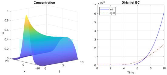
Let $L=20$ m, $T=10$ s, $a=5$ m²s⁻¹, $b=1$ ms⁻¹, $e=0.002$ s⁻¹, $x_0=5$ m and the concentration source be

$$f\left(t\right)=\left\{\begin{array}{cc}\hfill T,& {\displaystyle t\le \frac{T}{2},}\hfill \\ \hfill {\displaystyle 1-\frac{t}{T},}& {\displaystyle t>\frac{T}{2}.}\hfill \end{array}\right.$$

(31)

If $C_0\left(x\right)=10\mathsf{\Phi }\left(x\right|0,4)$ mgm⁻³, where $\mathsf{\Phi }\left(x\right|{\mu }_x,{\sigma }_x)$ is the PDF of the normal distribution with mean ${\mu }_x$ and standard deviation ${\sigma }_x$, then the solution to the localized problem (26) is plotted on Figure 1 (left), and the boundary conditions are given in Figure 1 (right).

Figure 1. Concentration (left) and boundary conditions (right) for problems (26)–(31).

Currently, we are able to start solving the inverse problem.

Let us take the measurements

$$C(x_1,t)=Y\left(t\right),0\le t\le T,$$

(32)

and, respectively,

$$u(x_1,t)=Y\left(t\right)\exp (-\beta t-\mu x_1)$$

(33)

for $x_1=0$.

The recovered function $f\left(t\right)$ (31) is presented in Figure 2. It relatively closely follows the true value (31).

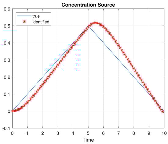
Figure 2. True and recovered values of the concentration source (31).

Let us try another experiment with a more fluctuating value of $f\left(t\right)$:

$$f\left(t\right)=\sin \left(t\right).$$

(34)

The identified source is given in Figure 3. Although lagging slightly, the recovered function follows the true trend.

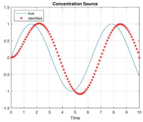
Figure 3. True and recovered values of the concentration source (34).

The same is true for the source, similar to [8]; see Figure 4.

$$f\left(t\right)=\left\{\begin{array}{cc}\hfill {\displaystyle \frac{2t}{T},}& {\displaystyle t\le \frac{T}{2},}\hfill \\ \hfill {\displaystyle 1,}& {\displaystyle t>\frac{T}{2}.}\hfill \end{array}\right.$$

(35)

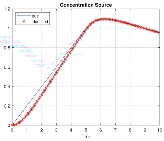
Figure 4. True and recovered values of the concentration source (35).

The suggested approach could also be successfully used as follows.

Example 2

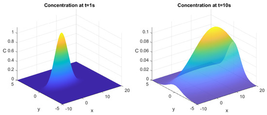
(An instantaneous injection at the origin into a uniform steady in an infinite plane). Let an amount M of pollutant be released instantaneously over a river with depth θ at $(x,y)=(0,0)$. The model is mathematically formulated as the following governing CDE,

$$\frac{\partial C}{\partial t}={\mathrm{D}}_L\frac{{\partial }^{2}C}{\partial x^2}+{\mathrm{D}}_T\frac{{\partial }^{2}C}{\partial y^2}-\mathrm{V}\frac{\partial C}{\partial x},$$

(36)

with initial conditions

$${\displaystyle {\left.C(x,y,t)\right|}_{t=0}=\frac{\mathrm{M}}{\theta }\delta (x,y),}$$

(37)

and boundary conditions

$$\begin{array}{c}{\left.C(x,y,t)\right|}_{x=\pm \infty }=0,t\ge 0,\hfill \\ {\left.C(x,y,t)\right|}_{y=\pm 0}=0,t\ge 0,\hfill \end{array}$$

where ${\mathrm{D}}_L$, ${\mathrm{D}}_T$, $\mathrm{V}$, $\mathrm{M}$ and θ are constants, and

$$C(x,y,t)=\frac{\mathrm{M}/\theta }{4\pi t\sqrt{{\mathrm{D}}_L{\mathrm{D}}_T}}\exp \left[-\frac{{(x-\mathrm{V}t)}^2}{4{\mathrm{D}}_{L}t}-\frac{y^2}{4{\mathrm{D}}_{T}t}\right].$$

Let us localize the domain as $\mathsf{\Omega }=\{-10\le x\le 20;-5\le y\le 5\}$ and $M=10$ gm⁻², $\theta =1$ m, ${\mathrm{D}}_L=5$ m²s⁻¹, ${\mathrm{D}}_T=0.1$ m²s⁻¹ and $V=1$ ms⁻¹. The measurements are taken at the point $(x_1,y_1)=(5,0)$.

The concentration is plotted at $t=1$ s and $t=10$ s in Figure 5.

Figure 5. Concentration at $t=1$ s (left) and $t=10$ s (right) for problem (36), (37).

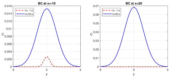
The boundary conditions at $x=-10$ and $x=20$ are given in Figure 6. The boundary conditions for $y=\pm 5$ are almost zero for all $t\le 10$ and are not interesting to plot.

Figure 6. Dirichlet boundary conditions at $x=-10$ m (left) and $x=20$ m (right) for problem (36), (37).

7. Conclusions

In this paper, we proposed efficient algorithms for solving Cauchy inverse problems with unknown sources. In the present study, using Green’s function method, we developed a procedure for constructing appropriate boundary conditions for a square domain such that the new problem preserves the properties of the original one, defined on an unbounded domain. Then, the time-dependent unknown source strength was reconstructed from point measurements inside the bounded domain.

We successfully applied the Tikhonov regularization method along with a first Fredholm integral equation to the inverse source problem. Test examples demonstrate that the proposed numerical method is efficient and accurate for the estimation of the unknown source on the base of point observations.

References

- Lenhart, S. Optimal control of a convective-diffusion fluid problems. Math. Model. Methods Appl. Sci. 1995, 5, 225–237. [Google Scholar] [CrossRef]
- Sun, N.Z. Mathematical Models of Growndwater Modeling; Kluwer: Dordrecht, The Netherlands, 1994. [Google Scholar]
- Genuchten, M.T.V.; Leij, F.J.; Skaggs, T.A.; Toride, N.; Bradford, S.A.; Pontedeiro, E.M. Exact analytical solutions for contaminant transport in rivers 1. The equilibrium advection-dispersion equation. J. Hydrol. Hydromech. 2013, 61, 146–160. [Google Scholar] [CrossRef]
- Guerro, J.S.; Pontdeiro, E.M.; van Genuchten, M.T.; Skaggs, T.H. Analytical solutions of the one-dimensional advection-dispersion solute transport equation subject to time-dependent boundary conditions. Chem. Eng. J. 2013, 221, 487–491. [Google Scholar] [CrossRef]
- Amirfakhrian, M.; Arghand, M.; Kansa, E.J. A new approximate method for an inverse time-dependent heat source problem using fundamental solutions and RBFs. Eng. Anal. Boundary Elem. 2016, 64, 278–289. [Google Scholar] [CrossRef]
- Erdem, A. A simultaneous approach to inverse source problem by Green’s function. Math. Methods Appl. Sci. 2015, 38, 1393–1401. [Google Scholar] [CrossRef]
- Pudykewicz, J.A. Application of adjoint tracer transport equations for evaluating source parameters. Atmos. Environ. 1998, 32, 3039–3050. [Google Scholar] [CrossRef]
- Shidarf, A.; Zakeri, A.; Neisi, A. A two-dimensinal inverse heat conduction problem for estimating heat source. Int. J. Math. Sci. 2005, 10, 1633–1641. [Google Scholar]
- Yan, L.; Fu, C.-L.; Yang, F.-L. The method of fundamental solutions for the inverse heat source problem. Eng. Anal. Bound. Elem. 2008, 32, 216–222. [Google Scholar] [CrossRef]
- Khairullin, M.H.; Shamsiev, M.N.; Sadovnikov, R. Algorithms for solution of the inverse coefficient problems of underground hydromechanics. Matem. Mod. 1998, 10, 101–110. [Google Scholar]
- Li, G.S.; Tan, Y.J.; Cheng, J.; Wang, X.Q. Determinating of grownwater pollution source by data compatibility analysis. Inverse Probl. Sci. Eng. 2006, 14, 287–300. [Google Scholar] [CrossRef]
- VNguyen, T.; Nguyen, H.T.; Tran, T.B.; Vo, A.K. On an inverse problem in the parabolic equation arising from groundwater pollution problem. Bound. Value Probl. 2015, 2015, 67. [Google Scholar]
- Georgiev, S.G.; Vulkov, L.G. Numerical solving of parabolic Cauchy problems by reduction on bounded domain and application to solute water pollution. AIP Conf. Proc. 2022, 2505, 080027. [Google Scholar]
- Badia, A.E.; Duong, T.H.; Hamdi, A. Identification a point source in a linear advection dispersion equation: Application to a pollution source problem. Inverse Problems 2005, 21, 1121–1136. [Google Scholar] [CrossRef]
- Li, H.; Wu, Y. Artificial boundary conditions for nonlnear time fractional Burger’s equation on unbounded domains. Appl. Math. Lett. 2021, 120, 107277. [Google Scholar] [CrossRef]
- Dang, Q.A.; Ehrhardt, M. Adequate numerical solution of air pollution problems by positive difference schemes on unbounded domains. Math. Comp. Model. 2006, 44, 834–856. [Google Scholar] [CrossRef]
- Han, H.D.; Huang, Z.Y. Exact and approximating boundary conditions for the parabolic problems on unbounded domain. Comput. Math. Appl. 2002, 44, 656–666. [Google Scholar] [CrossRef]
- Han, H.; Wu, X. Artificial Boundary Method; Springer: Berlin/Heidelberg, Germany, 2013. [Google Scholar]
- Valkov, R. Convergence of a finite volume element method for a generalized Black–Scholes equation transformed on a finite interval. Comp. Appl. Math. 2015, 16, 175–186. [Google Scholar] [CrossRef]
- Stakgold, I. Green’s Functions and Boundary Value Problems; Wiley: New York, NY, USA, 1979. [Google Scholar]
- Dautray, R.; Lions, J.-L. Mathematical Analysis and Numerical Methods for Science and Technology; Volume 1, Physical Origins and Classical Methods; Springer: Berlin/Heidelberg, Germany, 1990. [Google Scholar]
- Lamm, P.K.; Elden, L. Numerical solution of first-kind Volterra equations by sequential Tikhonov regularization. SIAM J. Numer. Anal. 1997, 34, 1432–1450. [Google Scholar] [CrossRef]
- Ryaben’kii, V.S.; Tsynkov, S.V. A Theoretical Introduction to Numerical Analysis; Chapman & Hall/CRC: Boca Raton, FL, USA, 2006. [Google Scholar]
- Samarskii, A. Theory of Difference Schemes; Marcel Dekker: New York, NY, USA, 2001. [Google Scholar]
Disclaimer/Publisher’s Note: The statements, opinions and data contained in all publications are solely those of the individual author(s) and contributor(s) and not of MDPI and/or the editor(s). MDPI and/or the editor(s) disclaim responsibility for any injury to people or property resulting from any ideas, methods, instructions or products referred to in the content. |
© 2023 by the authors. Licensee MDPI, Basel, Switzerland. This article is an open access article distributed under the terms and conditions of the Creative Commons Attribution (CC BY) license (https://creativecommons.org/licenses/by/4.0/).