On Predictive Modeling Using a New Three-Parameters Modification of Weibull Distribution and Application

Abstract

In this article, a new modification of the Weibull model with three parameters, the new exponential Weibull distribution (E-WD), is defined. The new model has many statistical advantages, the heavy-tailed behavior and the regular variation property were offered. Many of the important statistical functions of the modified model are presented in closed forms. The flexibility of E-WD has been improved. The proposed model can be used to fit data with different shapes, it can be right-skewed, left-skewed, decreasing, curved and symmetric. Some distribution properties of the proposed model, including moment generating function, characteristic function, moment, quantile and identifiability property, have been derived. In addition to the information generating function, the Shannon entropy and information energy are also discussed. The maximum likelihood approach and Bayesian estimation are used to estimate the distribution parameters. In the Bayesian method, three different loss functions are used. The calculations show the biases and estimated risks to obtain the best estimator. The bootstrap confidence intervals, the asymptotic confidence intervals and the observed variance-covariance matrix are obtained. Metropolis Hastings’ MCMC procedure is used for the calculations. We apply the composite distribution to stock data for four variables. The goodness-of-fit results show that the model performs well compared to its competitors. The proposed model can be used for forecasting and decision making.

1. Introduction

In this article, we present a new statistical distribution with three parameters that has some desirable properties. There are many previous studies and researches on the topic of composite distributions and the study of their properties, as well as methods for estimating the parameters and the reliability function. Here are some related researches and studies on this topic. Nadarajah and KOT [1] introduced a composite probability model, as he derived some of the characteristics of the proposed model represented by the probability distribution function, moments, mode, median, and the study of property measures of dispersion such as variance, average deviation, torsion, and flattening, and the parameters of the proposed model and the reliability function were estimated. Lingji et al. [2] develop a new composite statistical model Beta-Gamma, investigated the model properties, estimated the parameters and the risk function in different ways, and applied the model to real data in the health field. Akinsete et al. [3] discussed construction of a new composite statistical model for the Beta-Pareto distribution with four parameters and the study of the properties of the model, such as the arithmetic mean, mode, median, standard deviation, variance, skewness, and flatness, as well as the parameters and reliability of the model. Barreto et al. [4] discussed the study of a complex statistical model Beta-Generalised Exponential in terms of its mathematical properties and the derivation of rth degree moments.

A study on the complex distribution beta-Burr XII was published, in which the characteristics were derived by Paranaiba et al. [5]. A study on the construction of a composite statistical model for the Beta-Half Cauchy distribution was presented by Cardeior and Lemonts [6], such as the arithmetic mean and mode, and some properties of the dispersion measures. ALkadim and Boshi [7] published a paper that combined the exponential-Pareto distribution with two independent distributions, the Exponential and the Pareto distribution. The properties of the new distribution were studied in terms of the probability density function, the reliability function, the cumulative function, the risk function, and the use of the method of greatest likelihood to estimate the parameters. Gupta and Kundu [8] proposed the generalized exponential distribution and Nasiri [9] estimated the parameters via using different method in person of outlier.

Many literatures researched the issue of new statistical models based on the Weibull distribution. For example, Martinez et al. [10] developed the generalized modified Weibull distribution. Lee et al. [11] developed a beta Weibull model. Tahir et al. [12] developed a new Weibull-Pareto distribution. Emam developed the generalised Weibull-Weibull distribution [13]. Emam and Tashkandy [14] developed the generalised Arcsine-Kumaraswamy-X family of distributions by incorporating a trigonometric function, the Weibull claim model [15] using a class of claim distributions, the modified alpha-power Weibull-Weibull model [16], the generalised modified Weibull model [17] and the Khalil generalized Weibull distribution based on ranked set samples [18]. The exponential probability density function is:

$$\begin{array}{cc}\hfill f(\chi ;\psi )=\psi e^{-\chi \psi },& \chi \ge 0,\psi >0.\end{array}$$

(1)

Here $\psi >0$ is the inverse scale parameter. The exponential is:

$$\begin{array}{cc}\hfill F(\chi ;\psi )=1-e^{-\chi \psi },& \chi \ge 0,\psi >0.\end{array}$$

(2)

Next, the Weibull cumulative distribution function with two parameters takes the following form:

$$\begin{array}{c}\hfill G(\chi ;\lambda ,\theta )=1-e^{-\lambda {\chi }^{\theta }},\chi \ge 0;\lambda ,\theta >0.\end{array}$$

(3)

where $\chi \ge 0$, $\lambda >0$ is the scale parameter and $\theta >0$ is the shape parameter.

2. The E-WD

In this section we introduce a new combined statistical model and study its behavior. It is the E-WD with three agency parameters, which also consists of an exponential family and a Weibull distribution. The proposed model is superior to many previous distributions and proves its efficiency in modeling stock movement data in the stock market. The cumulative distribution function (CDF) of the new combined statistical model is as follows:

$$\begin{array}{ccc}\hfill F\left(\chi ;\psi ,\lambda ,\theta \right)& \hfill =\hfill & \hfill {\int }_0^{G(\chi ;\lambda ,\theta )}f(x;\psi )dx\hfill \\ \hfill & \hfill =\hfill & \hfill {\int }_0^{1-e^{\lambda {\chi }^{\theta }}}\psi e^{-x\psi }dx\hfill \\ \hfill & \hfill =\hfill & \hfill {\left[e^{-x\psi }\right]}_0^{1-e^{\lambda {\chi }^{\theta }}}\hfill \\ \hfill & \hfill =\hfill & \hfill 1-e^{-\left(1-e^{-\lambda {\chi }^{\theta }}\right)\psi }.\hfill \end{array}$$

(4)

The probability density function (PDF) of the complex statistical model gives as follows:

$$\begin{array}{ccc}\hfill f\left(\chi ;\psi ,\lambda ,\theta \right)& \hfill =\hfill & \hfill \frac{\partial F\left(\chi ;\psi ,\lambda ,\theta \right)}{\partial \chi }\hfill \\ \hfill & \hfill =\hfill & \hfill e^{\left(e^{-{\chi }^{\theta }\lambda }-1\right)\psi }{e}^{-{\chi }^{\theta }\lambda }{\chi }^{\theta -1}\psi \lambda \theta .\hfill \end{array}$$

(5)

$\forall \chi ;\lambda ,\theta ,$ and $\psi$, the function in the aforementioned Equation (5) $f\left(\chi ;\psi ,\lambda ,\theta \right)>0$, but

$$\begin{array}{ccc}\hfill {\int }_0^{\infty }f\left(\chi ;\psi ,\lambda ,\theta \right)d\chi & \hfill =\hfill & \hfill {\int }_0^{\infty }{e}^{\left(e^{-{\chi }^{\theta }\lambda }-1\right)\psi }{e}^{-{\chi }^{\theta }\lambda }{\chi }^{\theta -1}\psi \lambda \theta d\chi \hfill \\ \hfill & \hfill =\hfill & \hfill {\left[-e^{\left(e^{-{\chi }^{\theta }\lambda }-1\right)\psi }\right]}_0^{\infty }\hfill \\ \hfill & \hfill =\hfill & \hfill 1-e^{-\psi }.\hfill \end{array}$$

(6)

The function in Equation (5) is a non-probability PDF because its integral is not equal to one, so the appropriate method to convert it into a probability density function is to multiply it by the reciprocal of integration. The PDF of the proposed E-WD is:

$$\begin{array}{c}\hfill f\left(\chi ;\psi ,\lambda ,\theta \right)=\frac{e^{\left(e^{-{\chi }^{\theta }\lambda }-1\right)\psi -{\chi }^{\theta }\lambda }{\chi }^{\theta -1}\psi \lambda \theta }{1-e^{-\psi }},\chi \ge 0;\psi ,\lambda ,\theta >0.\end{array}$$

(7)

The corresponding CDF gives as follows:

$$\begin{array}{ccc}\hfill F\left(\chi ;\psi ,\lambda ,\theta \right)& \hfill =\hfill & \hfill {\int }_0^{\chi }f\left(u;\psi ,\lambda ,\theta \right)d\chi \hfill \\ \hfill & \hfill =\hfill & \hfill \frac{\psi \lambda \theta }{1-e^{-\psi }}{\int }_0^{\chi }{e}^{\left(-1+e^{-u^{\theta }\lambda }\right)\psi -u^{\theta }\lambda }{u}^{\theta -1}d\chi \hfill \\ \hfill & \hfill =\hfill & \hfill \frac{1}{1-e^{-\psi }}{\left[-e^{\left(-1+e^{-u^{\theta }\lambda }\right)\psi }\right]}_0^{\chi }.\hfill \end{array}$$

(8)

The CDF of E-WD is

$$\begin{array}{c}\hfill F\left(\chi ;\psi ,\lambda ,\theta \right)=\frac{1}{1-e^{-\psi }}\left[1-e^{\left(e^{-{\chi }^{\theta }\lambda }-1\right)\psi }\right],\chi \ge 0;\psi ,\lambda ,\theta >0.\end{array}$$

(9)

Furthermore, the survival function, hazard function, cumulative hazard function, and reverse hazard function of E-WD are given, respectively, by

$$\begin{array}{ccc}\hfill S\left(\chi ;\psi ,\lambda ,\theta \right)& =& \hfill 1-F\left(\chi ;\psi ,\lambda ,\theta \right)=\frac{e^{e^{-{\chi }^{\theta }\lambda }\psi }-1}{e^{\psi }-1},\hfill \\ \hfill \end{array}$$

(10)

$$\begin{array}{ccc}\hfill h\left(\chi ;\psi ,\lambda ,\theta \right)& =& \hfill \frac{f\left(\chi ;\psi ,\lambda ,\theta \right)}{S\left(\chi ;\psi ,\lambda ,\theta \right)}=\frac{e^{e^{-{\chi }^{\theta }\lambda }\psi -{\chi }^{\theta }\lambda }{\chi }^{\theta -1}\psi \lambda \theta }{e^{e^{-{\chi }^{\theta }\lambda }\psi }-1},\hfill \\ \hfill \end{array}$$

(11)

$$\begin{array}{ccc}\hfill H\left(\chi ;\psi ,\lambda ,\theta \right)& =& \hfill -\mathrm{Log}\left[F\right]=-\mathrm{Log}\left[\frac{e^{\psi }-e^{e^{-{\chi }^{\theta }\lambda }\psi }}{e^{\psi }-1}\right],\hfill \\ \hfill \end{array}$$

(12)

$$\begin{array}{ccc}\hfill r\left(\chi ;\psi ,\lambda ,\theta \right)& =& \hfill \frac{f\left(\chi ;\psi ,\lambda ,\theta \right)}{F\left(\chi ;\psi ,\lambda ,\theta \right)}=\frac{e^{e^{-{\chi }^{\theta }\lambda }\psi -{\chi }^{\theta }\lambda }{\chi }^{\theta -1}\psi \lambda \theta }{e^{\psi }-e^{e^{-{\chi }^{\theta }\lambda }\psi }}.\hfill \end{array}$$

(13)

The importance and main motivation for the proposed modification E-WD:

(i)

To improve the flexibility and distribution properties of Weibull model.

(ii)

The proposed model can take several forms: a right-skewed form, a left-skewed form, a decreasing form, a curved form, and a symmetric form.

(iii)

A simple way to add an additional parameter that gives an extended distribution with “heavy tail” properties and is very useful in modeling stock movement data and financial data.

(iv)

The important statistical functions of the modified E-WD are presented in closed forms.

(v)

The new version has many special statistical features. Now we present the visual representation of the PDF of the E-WD.

Various visual representations of the E-WD PDF are shown in Figure 1. The representations of f(x) are obtained for $0\le \chi \le 2$ and for; (i) $\lambda =0.2, \theta =0.8, \psi =2.4$ (blue-line), (ii) $\lambda =0.2, \theta =1.8, \psi =2.4$ (green-line), (iii) $\lambda =0.2, \theta =0.8, \psi =1.5$ (orange-line), (vi) $\lambda =1.2, \theta =0.8, \psi =1.5$ (red-line). In Figure 1, the representations of f(x) are obtained for $0\le \chi \le 2$ and for; (i) $\lambda =0.5, \theta =0.5, \psi =3.8$ (blue-line), (ii) $\lambda =0.5, \theta =0.5, \psi =3.8$ (green-line), (iii) $\lambda =2.3, \theta =0.5, \psi =3.8$ (orange-line), (vi) $\lambda =0.05, \theta =0.06, \psi =3.8$ (red-line). In left banal of Figure 1 we can observe the different shapes of the PDF of the E-WD. These include a right-skewed shape (green line), a decreasing shape (orange line), a curved shape (red line), zero skewness and a symmetrical shape (blue line). In right banal of Figure 1 we can observe the different shapes of the PDF of the E-WD. These include a left-skewed shape (red line), a decreasing shape (green line), and a symmetrical shape (blue line and orange line). From Figure 1, we can see that the E-WD PDF is very flexible and therefore can be used to cover datasets with indicated, decreasing, right-skewed, left-skewed or symmetric behaviour. Figure 2 presents the CDF of the corresponding casses of Figure 1.

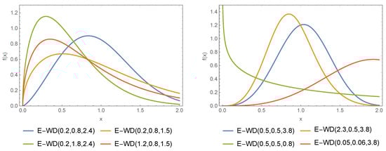
Figure 1. Different PDF for the E-WD.

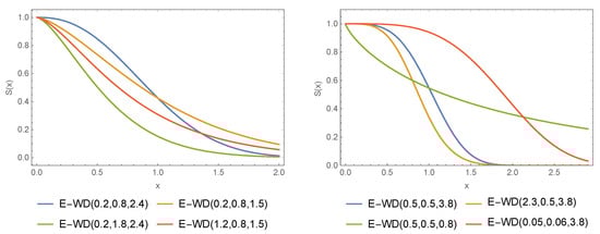
Figure 2. Different CDF for the E-WD.

3. The Heavy-Tailed Characteristic

This section offers the heavy-tailed behavior and regular variational results of the E-WD. Probability distributions that are right-skewed and possess heavy-tailed behavior are very useful in providing the best description of the biomedical data sets. A probability model is called a heavy tailed distribution, if it satisfies for every p

$$\begin{array}{c}\hfill \underset{y\to \infty }{\lim }S\left(y,\psi ,\lambda ,\theta \right)e^{p\chi }\to \infty .\end{array}$$

(14)

Theorem 1. 

$\forall p,\psi ,\lambda ,\theta >0$, the probability distribution $f\left(y,\psi ,\lambda ,\theta \right)$ that given in Equation (5) is heavy tailed distribution as $y\to \infty$.

Proof. 

Based on Equation (10), we can write that

$$\begin{array}{ccc}\hfill \underset{y\to \infty }{\lim }S\left(y,\psi ,\lambda ,\theta \right)e^{p\chi }& \hfill =\hfill & \hfill \underset{y\to \infty }{\lim }{e}^{py}\left(\frac{e^{e^{-y^{\theta }\lambda }\psi }-1}{e^{\psi }-1}\right)\hfill \\ \hfill & \hfill =\hfill & \hfill \frac{\underset{y\to \infty }{\lim }{e}^{-\left(2-e^{-\lambda y^{\theta }}\right)\psi +py}}{1-e^{-\psi }}\hfill \\ \hfill & \hfill =\hfill & \hfill \frac{e^{-(2-0)\psi +p\infty }}{1-e^{-\psi }}\hfill \\ \hfill & \hfill =\hfill & \hfill \frac{e^{\infty }}{1-e^{-\psi }}\to \infty .\hfill \end{array}$$

(15)

□

An important property of the heavy-tailed probability distributions is called the regular variational property. This property implies that the tail of the distribution decays in a power-law fashion, with an exponent $\Delta$ that determines how fast it decays. The larger the value of $\Delta$, the slower the decay of the tail. The regular variational property has important implications for many areas of science and engineering, including finance, telecommunications, and network science. It allows us to model extreme events and rare occurrences more accurately and to estimate their probabilities more reliably. Here, we derive the regular variational property of the E-WD. According to Karamata’s theorem (see, Seneta [19]), the E-WD in terms of SF $S\left(y,\psi ,\lambda ,\theta \right)$ is regularly varying, if it satisfies for every p

$$\begin{array}{c}\hfill \underset{y\to \infty }{\lim }\frac{S\left(py,\psi ,\lambda ,\theta \right)}{S\left(y,\psi ,\lambda ,\theta \right)}=p^{\Delta },\forall p,\Delta >0.\end{array}$$

(16)

where $\Delta$ represents an index of regular variation.

Theorem 2. 

$\forall p,\theta >0$, non-zero and finite, the probability distribution $f\left(y,\psi ,\lambda ,\theta \right)$ that given in Equation (5) is regularly varying model.

Proof. 

Using Equation (10), we can write that

$$\begin{array}{ccc}\hfill \frac{S\left(py,\psi ,\lambda ,\theta \right)}{S\left(y,\psi ,\lambda ,\theta \right)}& \hfill =\hfill & \hfill \frac{1-\frac{1-e^{-\left(1-e^{-\lambda {\left(py\right)}^{\theta }}\right)\psi }}{1-e^{-\psi }}}{1-\frac{1-e^{-\left(1-e^{-\lambda y^{\theta }}\right)\psi }}{1-e^{-\psi }}}\hfill \\ \hfill & \hfill =\hfill & \hfill \frac{1-e^{{\left(e^{-y^{\theta }\lambda }\psi \right)}^{p^{{\delta }_2}}}}{1-e^{e^{-y^{\theta }\lambda }\psi }}.\hfill \end{array}$$

(17)

Now, we can write

$$\begin{array}{c}\hfill \underset{y\to \infty }{\lim }\frac{1-e^{{\left(e^{-y^{\theta }\lambda }\psi \right)}^{p^{\theta }}}}{1-e^{e^{-y^{{\delta }_2}\lambda }\psi }}=\underset{x\to 1}{\lim }\frac{1-x^{p^{\theta }}}{1-x}=p^{\theta }.\end{array}$$

(18)

□

The expression in Equation (18) is non-zero and finite $\forall p,\theta >0$. Thus, $f\left(y,\psi ,\lambda ,\theta \right)$ that given in Equation (5) is a regular varying distribution and $\theta$ is the index of regular variation.

4. Distributional Properties

Here we derive some distribution properties of the E-WD. These distribution properties include the quantile function, the rth moment, the moment generating function (MG-F), the characteristic function (C-F), and the identifiability property (I-P).

4.1. The Quantile Function

By inverting Equation (9), we get the form of the quantile function of the E-WD expressed as

$$\begin{array}{c}\hfill {\chi }_p={\left(-\frac{\lambda }{Z}\right)}^{-1/\theta },\end{array}$$

(19)

where $Z=\mathrm{Log}\left[\frac{\mathrm{Log}\left[e^{\psi }+u-e^{\psi }u\right]}{\psi }\right]$. These quartiles can be used to derive further properties of the E-WD such as (i) skewness (see Bowley [20]) and (ii) kurtosis (See, Moor [21]). Figure 3 plots the skewness and kurtosis of the model $E-WD(1.2,0.6,0.9)$. The skewness and kurtosis formulas are, respectively, given by

$$S_K=\frac{2{\chi }_{1/2}-{\chi }_{3/4}-{\chi }_{1/4}}{{\chi }_{1/4}-{\chi }_{3/4}},$$

and,

$$K=\frac{{\chi }_{1/8}-{\chi }_{3/8}+{\chi }_{5/8}-{\chi }_{7/8}}{{\chi }_{2/8}-{\chi }_{6/8}}.$$

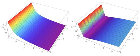
Figure 3. Plots for the skewness and kurtosis of E-WD.

4.2. The rth Moment

Suppose $\chi$ is a random vaiable follows the E-WD, then, its rth moment is obtained as

$$\begin{array}{ccc}\hfill {\mu }_r^{\prime }& \hfill =\hfill & \hfill E\left({\chi }^r\right)={\int }_0^{\infty }{\chi }^{r}f\left(y,\psi ,\lambda ,\theta \right)d\chi \hfill \\ \hfill & \hfill =\hfill & \hfill \frac{\psi \lambda \theta }{e^{\psi }-1}{\int }_0^{\infty }{e}^{e^{-{\chi }^{\theta }\lambda }\psi }{e}^{-{\chi }^{\theta }\lambda }{\chi }^{-1+\theta +r}d\chi .\hfill \end{array}$$

(20)

By using Maclaurin series expansion for $e^{e^{-{\chi }^{\theta }\lambda }\psi }={\sum }_{\delta =0}^{\infty }\frac{{\psi }^{\delta }}{\delta !}{e}^{-{\chi }^{\theta }\lambda \delta }$, we can write

$$\begin{array}{ccc}\hfill {\mu }_r^{\prime }& \hfill =\hfill & \hfill \frac{\psi \lambda \theta }{e^{\psi }-1}{\int }_0^{\infty }{\displaystyle \sum _{\delta =0}^{\infty }}\frac{{\psi }^{\delta }}{\delta !}{e}^{-{\chi }^{\theta }\lambda \delta }{e}^{-{\chi }^{\theta }\lambda }{\chi }^{\theta +r-1}d\chi \hfill \\ \hfill & \hfill =\hfill & \hfill \frac{\psi \lambda \theta }{e^{\psi }-1}{\displaystyle \sum _{\delta =0}^{\infty }}\frac{{\psi }^{\delta }}{\delta !}{\int }_0^{\infty }{e}^{-{\chi }^{\theta }\lambda (\delta +1)}{\chi }^{\theta +r-1}d\chi \hfill \\ \hfill & \hfill =\hfill & \hfill \frac{\psi \lambda }{e^{\psi }-1}{\displaystyle \sum _{\delta =0}^{\infty }}\frac{{\psi }^{\delta }}{\delta !}I\left(\delta \right),\hfill \end{array}$$

(21)

where $I\left(\delta \right)={\left((1+\delta )\lambda \right)}^{-\frac{r+\theta }{\theta }}\Gamma \left[\frac{r+\theta }{\theta }\right].$

4.3. The MG-F

The MG-F of the E-WD is derived as

$$\begin{array}{ccc}\hfill M_t\left(\chi \right)& \hfill =\hfill & \hfill E\left(e^{tx}\right)={\int }_0^{\infty }{e}^{tx}f\left(\chi ;\psi ,\lambda ,\theta \right)d\chi \hfill \\ \hfill & \hfill =\hfill & \hfill \frac{\psi \lambda \theta }{e^{\psi }-1}{\int }_0^{\infty }{e}^{e^{-{\chi }^{\theta }\lambda }\psi }{e}^{tx-{\chi }^{\theta }\lambda }{\chi }^{\theta -1}d\chi \hfill \\ \hfill & \hfill =\hfill & \hfill \frac{\psi \lambda \theta }{e^{\psi }-1}{\displaystyle \sum _{\delta =0}^{\infty }}\frac{{\psi }^{\delta }}{\delta !}{\int }_0^{\infty }{e}^{-{\chi }^{\theta }\lambda \delta }{e}^{tx-{\chi }^{\theta }\lambda }{\chi }^{\theta -1}d\chi .\hfill \end{array}$$

(22)

And by expanding $e^{tx}={\sum }_{\zeta =0}^{\infty }\frac{t^{\zeta }}{\zeta !}{x}^{\zeta }$, we can write

$$\begin{array}{ccc}\hfill M_t\left(\chi \right)& \hfill =\hfill & \hfill \frac{\psi \lambda \theta }{e^{\psi }-1}{\displaystyle \sum _{\delta =0}^{\infty }}\frac{{\psi }^{\delta }}{\delta !}{\displaystyle \sum _{\zeta =0}^{\infty }}\frac{t^{\zeta }}{\zeta !}{\int }_0^{\infty }{e}^{-{\chi }^{\theta }\lambda (1+\delta )}{x}^{-1+\theta +\zeta }d\chi \hfill \\ \hfill & \hfill =\hfill & \hfill \frac{\psi \lambda }{e^{\psi }-1}{\displaystyle \sum _{\delta =0}^{\infty }}\frac{{\psi }^{\delta }}{\delta !}{\displaystyle \sum _{\zeta =0}^{\infty }}\frac{t^{\zeta }}{\zeta !}{\left((1+\delta )\lambda \right)}^{-\frac{\zeta +\theta }{\theta }}\mathsf{\Gamma }\left[\frac{\zeta +\theta }{{\delta }_2}\right],\hfill \end{array}$$

(23)

where $\mathsf{\Gamma }$ is a gamma constant.

4.4. The C-F

The C-F ${\varphi }_{\mathrm{it}}\left(\chi \right)$ is another useful approach for obtaining the basic moments of a probability model. Here, we can write

$$\begin{array}{ccc}\hfill {\varphi }_{\mathrm{it}}\left(\chi \right)& \hfill =\hfill & \hfill E\left(e^{it\chi }\right)\hfill \\ \hfill & \hfill =\hfill & \hfill {\int }_0^{\infty }{e}^{it\chi }\frac{e^{e^{-{\chi }^{\theta }\lambda }\psi -{\chi }^{\theta }\lambda }{\chi }^{\theta -1}\psi \lambda \theta }{e^{\psi }-1}d\chi .\hfill \end{array}$$

(24)

The C-F of the E-WD can take the form

$$\begin{array}{ccc}\hfill {\varphi }_{\mathrm{it}}\left(\chi \right)& =& \hfill E\left(e^{it\chi }\right)=\frac{\psi \lambda }{e^{\psi }-1}{\displaystyle \sum _{\delta =0}^{\infty }}\frac{{\psi }^{\delta }}{\delta !}{\displaystyle \sum _{\zeta =0}^{\infty }}\frac{{\left(it\right)}^{\zeta }}{\zeta !}{\left((1+\delta )\lambda \right)}^{-\frac{\zeta +\theta }{\theta }}\mathsf{\Gamma }\left[\frac{\zeta +\theta }{{\delta }_2}\right].\hfill \end{array}$$

(25)

4.5. The I-P

This subsection offers proof of the I-P of the E-WD for the parameters.

4.5.1. The I-P Using $\lambda$

Here, we provide complete proof of the IP of the E-WD for $\lambda$. Suppose ${\lambda }_1$ and ${\lambda }_2$ be the parameters of the E-WD with CDFs

$$\begin{array}{c}\hfill F_1\left(y\right)=\frac{1-e^{-\left(1-e^{-{\lambda }_1{\chi }^{\theta }}\right)\psi }}{1-e^{-\psi }},\mathrm{and}{F}_2\left(y\right)=\frac{1-e^{-\left(1-e^{-{\lambda }_2{\chi }^{\theta }}\right)\psi }}{1-e^{-\psi }}.\end{array}$$

(26)

respectively. The parameter $\lambda$ of the E-WD is called identifiable, if ${\lambda }_1={\lambda }_2$. To prove the I-P of the E-WD for $\lambda$, we start with

$$\begin{array}{ccc}\hfill \frac{1-e^{-\left(1-e^{-{\lambda }_1{\chi }^{\theta }}\right)\psi }}{1-e^{-\psi }}& \hfill =\hfill & \hfill \frac{1-e^{-\left(1-e^{-{\lambda }_2{\chi }^{{\delta }_2}}\right)\psi }}{1-e^{-\psi }},\hfill \\ \hfill -\left(1-e^{-{\lambda }_1{\chi }^{\theta }}\right)\psi & \hfill =\hfill & \hfill -\left(1-e^{-{\lambda }_2{\chi }^{\theta }}\right)\psi ,\hfill \\ \hfill e^{-{\lambda }_1{\chi }^{\theta }}& \hfill =\hfill & \hfill e^{-{\lambda }_2{\chi }^{\theta }},\hfill \\ \hfill {\lambda }_1& \hfill =\hfill & \hfill {\lambda }_2.\hfill \end{array}$$

(27)

4.5.2. The I-P Using $\theta$

Let ${\theta }_1$ and ${\theta }_2$ be the parameters of the E-WD with CDFs

$$\begin{array}{c}\hfill F_1\left(y\right)=\frac{1-e^{-\left(1-e^{-\lambda {\left(\chi \right)}^{{\theta }_1}}\right)\psi }}{1-e^{-\psi }},\mathrm{and}{F}_2\left(y\right)=\frac{1-e^{-\left(1-e^{-\lambda {\left(\chi \right)}^{{\theta }_2}}\right)\psi }}{1-e^{-\psi }}.\end{array}$$

(28)

respectively. The parameter $\theta$ of the E-WD is called identifiable, if ${\theta }_1={\theta }_2$. To prove the I-P of the E-WD for a1, we start with

$$\begin{array}{ccc}\hfill \frac{1-e^{-\left(1-e^{-\lambda {\left(\chi \right)}^{{\theta }_1}}\right)\psi }}{1-e^{-\psi }}& \hfill =\hfill & \hfill \frac{1-e^{-\left(1-e^{-\lambda {\left(\chi \right)}^{{\delta }_{2}2}}\right)\psi }}{1-e^{-\psi }},\hfill \\ \hfill -\left(1-e^{-\lambda {\left(\chi \right)}^{{\theta }_1}}\right)\psi & \hfill =\hfill & \hfill -\left(1-e^{-\lambda {\left(\chi \right)}^{{\theta }_2}}\right)\psi ,\hfill \\ \hfill {\theta }_1& \hfill =\hfill & \hfill {\theta }_2.\hfill \end{array}$$

(29)

4.5.3. The IP Using $\psi$

Let ${\psi }_1$ and ${\psi }_2$ be the parameters of the E-WD with CDFs

$$\begin{array}{c}\hfill F_1\left(y\right)=\frac{1-e^{-\left(1-e^{-\lambda {\chi }^{\theta }}\right){\psi }_1}}{1-e^{-{\psi }_1}},\mathrm{and}{F}_2\left(y\right)=\frac{1-e^{-\left(1-e^{-\lambda {\chi }^{\theta }}\right){\psi }_2}}{1-e^{-{\psi }_2}}.\end{array}$$

(30)

respectively. The parameter $\psi$ of the E-WD is called identifiable, if ${\psi }_1={\psi }_2$. To prove the I-P of the E-WD for a1, we start with

$$\begin{array}{ccc}\hfill \frac{1-e^{-\left(1-e^{-\lambda {\chi }^{\theta }}\right){\psi }_1}}{1-e^{-\psi }}& \hfill =\hfill & \hfill \frac{1-e^{-\left(1-e^{-\lambda {\chi }^{{\delta }_2}}\right){\psi }_2}}{1-e^{-\psi }},\hfill \\ \hfill \left(1-e^{-\lambda {\chi }^{\theta }}\right){\psi }_1& \hfill =\hfill & \hfill \left(1-e^{-\lambda {\chi }^{\theta }}\right){\psi }_2,\hfill \\ \hfill {\psi }_1& \hfill =\hfill & \hfill {\psi }_2.\hfill \end{array}$$

(31)

5. The Information Generating Measure

In addition to the moment generating function, information generating functions (IGF) have also been used in information theory, to generate some well-known information measures such as Shannon entropy and Kullback–Leibler divergence. For more details about the IGF and its extensions one may see López-Ruiz et al. [22].

5.1. The Information Generating Function

Let X∼$f\left(\chi \right)$, the information generating function ${\mathsf{\Omega }}_{\gamma }\left(\chi \right)$, for any $\gamma >0$ (see, Golomb [23]), is defined as

$$\begin{array}{ccc}\hfill {\mathsf{\Omega }}_{\gamma }\left(\chi \right)& \hfill =\hfill & \hfill {\int }_0^{\infty }{f}^{\gamma }\left(\chi ;\psi ,\lambda ,\theta \right)d\chi \hfill \\ \hfill & \hfill =\hfill & \hfill {\int }_0^{\infty }{\left(\frac{e^{e^{-{\chi }^{\theta }\lambda }\psi -{\chi }^{\theta }\lambda }{\chi }^{\theta -1}\psi \theta {\delta }_1}{e^{\psi }-1}\right)}^{\gamma }d\chi \hfill \\ \hfill & \hfill =\hfill & \hfill {\left(\frac{\psi \lambda \theta }{e^{\psi }-1}\right)}^{\gamma }{\int }_0^{\infty }{e}^{\gamma e^{-{\chi }^{\theta }\lambda }\psi }{e}^{-{\chi }^{\theta }\lambda \gamma }{x}^{\left(-1+\theta \right)\gamma }d\chi \hfill \\ \hfill & \hfill =\hfill & \hfill {\left(\frac{\psi \lambda \theta }{e^{\psi }-1}\right)}^{\gamma }{\displaystyle \sum _{\delta =0}^{\infty }}\frac{{\left(\gamma \psi \right)}^{\delta }}{\delta !}{\int }_0^{\infty }{e}^{-{\chi }^{\theta }\lambda (\gamma +\delta )}{x}^{\left(-1+\theta \right)\gamma }d\chi \hfill \\ \hfill & \hfill =\hfill & \hfill {\left(\frac{\psi \lambda \theta }{e^{\psi }-1}\right)}^{\gamma }{\displaystyle \sum _{\delta =0}^{\infty }}\frac{{\left(\gamma \psi \right)}^{\delta }}{\delta !\theta }{\left((\gamma +\delta )\lambda \right)}^{\frac{-1+\gamma -\gamma \theta }{\theta }}\mathsf{\Gamma }\left[\frac{1+\gamma \left(-1+\theta \right)}{\theta }\right].\hfill \end{array}$$

(32)

5.2. The Shannon Entropy (H)

The Shannon entropy, or Information entropy was introduced by Claude Shannon [24], and is defined as

$$\begin{array}{c}\hfill H=-{\int }_{X}f\left(\chi \right)log\left(f\left(\chi \right)\right)d\chi .\end{array}$$

(33)

H can obtain from ${\mathsf{\Omega }}_{\gamma }\left(\chi \right)$ as

$$\begin{array}{c}\hfill H={\left.-\frac{\partial {\mathsf{\Omega }}_{\gamma }\left(\chi \right)}{\partial \gamma }\right|}_{\gamma =1}.\end{array}$$

(34)

$$\begin{array}{ccc}\hfill H=& \hfill -\hfill & \hfill \left(\mathrm{Log}\left[\frac{\psi \lambda \theta }{e^{\psi }-1}\right]+\frac{1}{\gamma }\right){\mathsf{\Omega }}_{\gamma }\left(\chi \right)+{\left(\frac{\psi \lambda \theta }{e^{\psi }-1}\right)}^{\gamma }{\displaystyle \sum _{\delta =0}^{\infty }}\frac{{\left(\psi \gamma \right)}^{\delta }}{\theta \delta !}\mathsf{\Gamma }\left[\frac{1+\gamma \left(-1+\theta \right)}{{\delta }_2}\right]\hfill \\ \hfill & \hfill \times \hfill & \hfill \left(-\lambda {\left((\gamma +\delta )\lambda \right)}^{-1+\frac{-1+\gamma -\gamma \theta }{\theta }}\left(\gamma +\frac{1+\gamma }{\theta }\right)\right.\hfill \\ \hfill & \hfill -\hfill & \hfill \left(1+\frac{1}{\theta }\right){\left(\lambda (\gamma +\delta )\right)}^{\frac{-1+\gamma -\gamma \theta }{\theta }}\mathrm{Log}\left[(\gamma +\delta )\lambda \right]\hfill \\ \hfill & \hfill +\hfill & \hfill \frac{{\left(\psi \gamma \right)}^{\delta }\left(-1+\theta \right){\left((\gamma +\delta )\lambda \right)}^{\frac{-1+\gamma -\gamma {\delta }_2}{\theta }}{\mathsf{\Gamma }}^{\prime }\left[\frac{1+\gamma \left(-1+{\delta }_2\right)}{\theta }\right]}{{\theta }^2\delta !}.\hfill \end{array}$$

(35)

5.3. The Informational Energy (IE)

The IE for any X∼$f\left(x\right)$, is given by

$$\begin{array}{c}\hfill IE=-{\int }_X{f}^2\left(\chi ;\psi ,\lambda ,\theta \right)d\chi .\end{array}$$

(36)

In particular, ${\mathsf{\Omega }}_{\gamma }\left(\chi \right)$ is simply IE when $\gamma =2$, and is given by

$$\begin{array}{c}\hfill IE=\theta {\left(\frac{\psi \lambda }{e^{\psi }-1}\right)}^2{\displaystyle \sum _{\delta =0}^{\infty }}\frac{2^{\delta }{\psi }^{\delta }}{\delta !}{\left((2+\delta )\lambda \right)}^{\frac{1-2\theta }{\theta }}\mathsf{\Gamma }\left[\frac{1+2\left(-1+\theta \right)}{\theta }\right].\end{array}$$

(37)

For some discussions on the usefulness and applications of the IE, see, Cataron and Andonie [25].

6. Maximum Likelihood Estimation (MLE)

Let ${\chi }_1,{\chi }_2,\dots ,{\chi }_n$ are observed values of $X_{1:n},X_{2:n},\cdots X_{n:n}$ that is an ordered random sample from the E-WD. The E-WD likelihood is

$$\begin{array}{c}\hfill l={\left(\frac{\psi \lambda \theta }{e^{\psi }-1}\right)}^n\left(\prod _{i=1}^n{\chi }_i^{-1+\theta }\right)e^{{\sum }_{i=1}^n\left(e^{-{\chi }_i^{\theta }\lambda }\psi -{\chi }_i^{\theta }\lambda \right)},\end{array}$$

(38)

and the corresponding log-likelihood function $\left(L\right)$ is

$$\begin{array}{c}\hfill L=n\mathrm{Log}\left[\frac{\psi \lambda \theta }{e^{\psi }-1}\right]+\sum _{i=1}^n\mathrm{Log}\left[{\chi }_i^{-1+\theta }\right]+\sum _{i=1}^n\left(e^{-{\chi }_i^{\theta }\lambda }\psi -{\chi }_i^{\theta }{\delta }_1\right),\end{array}$$

(39)

Taking the first partial derivatives of log-likelihood (39) with respect to $\psi ,\lambda ,\theta$ and equating each to zero.

$$\begin{array}{ccc}\hfill \frac{\partial }{\partial \psi }L& =& \hfill \frac{n\left(e^{\psi }-1\right)}{\psi \lambda \theta }\left(\frac{{\delta }_2\lambda }{e^{\psi }-1}-\frac{e^{\psi }\psi \lambda \theta }{{\left(e^{\psi }-1\right)}^2}\right)+\sum _{i=1}^n{e}^{-\lambda {\chi }_i^{\theta }}=0,\hfill \\ \hfill \end{array}$$

(40)

$$\begin{array}{ccc}\hfill \frac{\partial }{\partial \theta }L& =& \hfill \frac{n}{\theta }+\sum _{i=1}^n\mathrm{Log}\left[{\chi }_i\right]+\sum _{i=1}^n\left(-\lambda \mathrm{Log}\left[{\chi }_i\right]{\chi }_i^{\theta }-e^{-\lambda {\chi }_i^{\theta }}\psi \lambda \mathrm{Log}\left[{\chi }_i\right]{\chi }_i^{{\delta }_2}\right)=0,\hfill \\ \hfill \end{array}$$

(41)

$$\begin{array}{ccc}\hfill \frac{\partial }{\partial \lambda }L& =& \hfill \frac{n}{\lambda }+\sum _{i=1}^n\left(-{\chi }_i^{\theta }-e^{-\lambda {\chi }_i^{\theta }}\psi {\chi }_i^{\theta }\right)=0.\hfill \end{array}$$

(42)

Solving Equation (42) for $\psi$, we have

$$\begin{array}{c}\hfill \psi =\frac{\frac{n}{\lambda }-{\sum }_{i=1}^n{\chi }_i^{\theta }}{{\sum }_{i=1}^n{e}^{-\lambda {\chi }_i^{\theta }}{\chi }_i^{\theta }}.\end{array}$$

(43)

Solving Equations (40) and (41) after substituting Equation (43), we get the maximum likelihood estimators ${\widehat{\psi }}_{ML},{\widehat{\lambda }}_{ML},{\widehat{\theta }}_{ML}$ of the $E-WD(\psi ,\lambda ,\theta )$ parameters.

The asymptotic confidence intervals of the parameters $\psi$, $\lambda$ and $\theta$. Then $\widehat{V}=V({\widehat{\psi }}_{ML},{\widehat{\lambda }}_{ML},{\widehat{\theta }}_{ML})=\left[{\sigma }_{i,j}\right],i,j=1,2,3$ is the observed variance covariance matrix, such that

$$\begin{array}{c}\hfill V(\psi ,\lambda ,\theta )=-{\left[\begin{array}{c}\hfill {\displaystyle \frac{{\partial }^{2}L}{\partial {\psi }^2}\frac{{\partial }^{2}L}{\partial \psi \partial \lambda }\frac{{\partial }^{2}L}{\partial \psi \partial \theta }}\hfill \\ \\ \hfill {\displaystyle \frac{{\partial }^{2}L}{\partial \lambda \partial \psi }\frac{{\partial }^{2}L}{\partial {\lambda }^2}\frac{{\partial }^{2}L}{\partial \lambda \partial \theta }}\hfill \\ \\ \hfill {\displaystyle \frac{{\partial }^{2}L}{\partial \theta \partial \psi }\frac{{\partial }^{2}L}{\partial \theta \partial \lambda }\frac{{\partial }^{2}L}{\partial {\theta }^2}}\hfill \end{array}\right]}^{-1},\end{array}$$

(44)

A $100(1-ϵ)\%$ two-sided approximate confidence intervals for the parameters $\psi$, $\lambda ,$ and $\theta$ are then given by

$$\widehat{\psi }\pm z_{ϵ/2}\sqrt{V(\widehat{\psi })},$$

(45)

$$\widehat{\lambda }\pm z_{ϵ/2}\sqrt{V(\widehat{\lambda })},$$

(46)

and

$$\widehat{\theta }\pm z_{ϵ/2}\sqrt{V(\widehat{\theta })},$$

(47)

respectively, where $V(\widehat{\psi }),$ $V(\widehat{\lambda }),$ and$V(\widehat{\theta }),$ are the estimated variances of ${\widehat{\psi }}_{ML}$, ${\widehat{\lambda }}_{ML}$, and ${\widehat{\theta }}_{ML}$, which are given by the diagonal elements of $\widehat{V}$, and $z_{ϵ/2}$ is the upper $\left(\frac{ϵ}{2}\right)$ percentile of the standard normal distribution.

Next, obtain the bootstrap confidence intervals for boot-p for the unknown parameters $\delta =(\psi ,\lambda ,\theta$), we apply the following algorithms

1.

Generate sample $\left\{{\chi }_i\right\}$ of size n from the $E-WD(\psi ,\lambda ,\theta )$ and estimate a $\widehat{\delta }$.

2.

Generate another sample $\left\{{\chi }_i^{*}\right\}$ of size n using $\widehat{\delta }$. Then estimate ${\widehat{\delta }}^{*}$.

3.

Repeat step 2 B times.

4.

Via $\widehat{F}(x)=P({\widehat{\delta }}^{*}\le x)$, that is, the CDF of ${\widehat{\delta }}^{*}$, the $100(1-ϵ)\%$ C.I. of $\delta$ is given by

$$\left({\widehat{\delta }}_{Boot-p}\left(\frac{ϵ}{2}\right),{\widehat{\delta }}_{Boot-p}(1-\frac{ϵ}{2})\right),$$

where ${\widehat{\delta }}_{Boot-p}\left(\kappa \right)={\widehat{F}}^{-1}\left(\kappa \right)$ and x is prefixed.

For more details about the bootstrap confidence intervals, one may refer to Kundu and Joarder [26].

7. Bayesian Estimation

Bayesian inference is a convenient method to be used with the complete samples from $E-WD(\psi ,\lambda ,\theta )$. We assume that $\psi$, $\lambda$, and $\theta$ are random variables that follow the prior PDFs Gamma$(\psi ;a_1,b_1)$, Gamma$(\lambda ;a_2,b_2)$, and Gamma$(\theta ;a_3,b_3)$, respectively, are given by

$$\begin{array}{c}\hfill {\pi }_1\left(\psi \right)=\frac{b_1^{{\alpha }_1}}{\mathsf{\Gamma }\left(a_1\right)}{\psi }^{a_1-1}exp\left[-b_1\psi \right],\psi ,a_1,b_1>0,\end{array}$$

(48)

$$\begin{array}{c}\hfill {\pi }_2\left(\lambda \right)=\frac{b_2^{a_2}}{\mathsf{\Gamma }\left(a_2\right)}{\lambda }^{a_2-1}exp\left[-b_2\lambda \right],\lambda ,a_2,b_2>0,\end{array}$$

(49)

and

$$\begin{array}{c}\hfill {\pi }_3\left(\theta \right)=\frac{b_3^{a_3}}{\mathsf{\Gamma }\left(a_3\right)}{\theta }^{a_3-1}exp\left[-b_3\theta \right],\theta ,a_3,b_3>0.\end{array}$$

(50)

Then, the posterior density of $\psi ,\lambda ,\theta$ and the data is given by

$$\begin{array}{c}\hfill {\pi }^{*}(\psi ,\lambda ,\theta |\mathbf{x})=J^{-1}\frac{{\psi }^{n+a_1-1}{\lambda }^{n+a_2-1}{\theta }^{n+a_3-1}}{{\left(1-e^{-\psi }\right)}^n}{e}^{{\sum }_{i=1}^n\left(e^{-{\chi }_i^{\theta }\lambda }-1\right)\psi -{\chi }_i^{\theta }\lambda }\prod _{i=1}^n{\chi }_i^{\theta -1},\end{array}$$

(51)

where J is the normalizing constant.

MCMC Method

We use Metropolis Hastings procedure as:

• Set start values ${\psi }^{\left(0\right)}$, ${\lambda }^{\left(0\right)}$, and ${\theta }^{\left(0\right)}$. Then, simulate sample of size n from E-WD $({\psi }^{\left(0\right)},{\lambda }^{\left(0\right)},{\theta }^{\left(0\right)})$, next set $l=1$.
• Simulate ${\psi }^{(*)},$${\lambda }^{(*)},$ and ${\theta }^{(*)}$. using the proposal distributions $N({\psi }^{(l-1)},V(\widehat{\psi }))$, $N({\lambda }^{(l-1)},V(\widehat{\lambda }))$, $N({\theta }^{(l-1)}$ and $V(\widehat{\theta }))$.
• Calculate $r=min\left(\frac{{\pi }^{*}({\psi }^{(*)},{\lambda }^{(*)},{\theta }^{(*)})}{{\pi }^{*}({\psi }^{(l-1)},{\lambda }^{(l-1)},{\theta }^{(l-1)})},1\right)$.
• Simulate U from Uniform(0, 1).
• If $U<r$, then $\left({\psi }^{\left(l\right)},{\lambda }^{\left(l\right)},{\theta }^{\left(l\right)}\right)=\left({\psi }^{(*)},{\lambda }^{(*)},{\theta }^{(*)}\right)$.
  If $U\ge r$, then $\left({\psi }^{(l-1)},{\lambda }^{(l-1)},{\theta }^{(l-1)}\right)=\left({\psi }^{(*)},{\lambda }^{(*)},{\theta }^{(*)}\right)$.
• Set $l=l+1$.
• Iterate Steps 2–6, M repetitions, and get ${\psi }^{\left(l\right)},{\lambda }^{\left(l\right)}$ and ${\theta }^{\left(l\right)}$ for $l=1,\cdots ,M$.

Suppose the squared error loss function, given by $L_{SE}(\delta ,\widehat{\delta })={(\delta -\widehat{\delta })}^2.$ By using the generated random samples from the M-H technique and for N is the nburn. Then, the Bayes estimator of $\delta$ against the squared error loss function, is given by

$$\begin{array}{c}\hfill {\widehat{\delta }}_{SE}=E_{\delta }\left[\delta |\mathbf{x}\right]=\frac{1}{M-N}{\displaystyle \sum _{l=N+1}^M}{\delta }^{\left(l\right)}.\end{array}$$

(52)

Next, suppose the LINEX ($LE$) loss function, given by

$$L_{LE}\left(\delta ,\widehat{\delta }\right)=exp\left[\rho \left(\delta -\widehat{\delta }\right)\right]-\rho \left(\delta -\widehat{\delta }\right)-1,\rho \ne 0.$$

(53)

The approximate Bayes estimate of $\delta$ under $LE$ loss function, is given by

$$\begin{array}{c}\hfill {\widehat{\delta }}_{LE}=\frac{-1}{\rho }log\left(E_{\delta }\left[exp\left(-\rho \delta \right)|\mathbf{x}\right]\right)=\frac{-1}{\rho }log\left(\frac{{\sum }_{l=N+1}^{M}exp\left(-\rho {\delta }^{\left(l\right)}\right)}{M-N}\right),\end{array}$$

(54)

Finally, suppose the general entropy ($GE$) loss function, given by

$$L_{GE}\left(\delta ,\widehat{\delta }\right)={\left(\frac{\widehat{\delta }}{\delta }\right)}^{\epsilon }-\epsilon log\left(\frac{\widehat{\delta }}{\delta }\right)-1.$$

(55)

The approximate Bayes estimate of the parameters, given by

$${\widehat{\delta }}_{GE}={\left.\left(E_{\delta }\left[{\delta }^{-\epsilon }\right|\mathbf{x}\right]\right)}^{\frac{-1}{\epsilon }}={\left(\frac{1}{M-N}\sum _{l=N+1}^M{\left({\delta }^{\left(l\right)}\right)}^{-\epsilon }\right)}^{\frac{-1}{\epsilon }},$$

(56)

MCMC HPD credible interval Algorithm:

• Arrange ${\psi }^{(*)},{\lambda }^{(*)}$ and ${\theta }^{(*)}$ in rising values.
• The lower bounds of ${\psi }^{(*)},{\lambda }^{(*)}$ and ${\theta }^{(*)}$ is in the rank $(M-N)*\epsilon /2$.
• The Upper bounds of ${\psi }^{(*)},{\lambda }^{(*)}$ and ${\theta }^{(*)}$ is in the rank $(M-N)*(1-\epsilon /2)$.
• Iterate the previous steps M times. Get the average value of the lower and upper bounds of $\psi ,\lambda ,$ and $\theta$.

8. Simulation Study

In this section, we show the usefulness of the theatrical findings in this paper by conducting series of simulation experiments. The simulations show the bias and estimated risk of bayesian and the maximum likelihood estimates. The biases and ERs are given, respectively, by

$$Bias\left(\widehat{\vartheta }\right)=\frac{1}{1000}\sum _{i=1}^{1000}\left({\widehat{\vartheta }}_i-\vartheta \right),$$

and

$$ER\left(\widehat{\vartheta }\right)=\frac{1}{1000}\sum _{i=1}^{1000}{\left({\widehat{\vartheta }}_i-\vartheta \right)}^2,$$

Coverage probabilities (CPs) are also calculated at the 95% and 90% HPD credible intervals. Point and Interval estimation of the parameters $\psi$, $\lambda$, and $\theta$ for n = 25, 50, and 100 are presented in Table 1. Table 2 represents the simulation results for the parameters $\psi$, $\lambda$ and $\theta$, respectively for n = 200, 300, and 400. The bayesian estimate are calculated based on GE, LINEX and SE loss functions. In addition, 95% and 90% the confidence, Bootstrap and HPD credible intervals are calculated with the corresponding width. The simulation experiments can be explained though the following steps:

Table 1. Point and Interval estimation of the parameters $\psi$, $\lambda$, and $\theta$ for n = 25, 50 and 100.

n	Par.	Point					Intrval
		$\mathit{ML}$	$\mathit{SE}$	$\mathit{LE}\mathbf{1}$	$\mathit{LE}\mathbf{2}$	$\mathit{GE}$	$\mathit{ML}$	$\mathit{Bootstrap}$	${\mathit{HPD}}_{\mathit{SE}}$	${\mathit{HPD}}_{\mathit{LE}\mathbf{1}}$	${\mathit{HPD}}_{\mathit{LE}\mathbf{2}}$	${\mathit{HPD}}_{\mathit{GE}}$
25	$\psi$	1.7182	2.8685	2.8712	2.8616	2.8631	0.0001 7.4805	1.718 1.718	2.751 2.98	2.7558 2.9802	2.7374 2.9802	2.7394 2.9802
		−0.7958	0.3545	0.3572	0.3477	0.3492	7.4804	0.0001	0.229	0.2244	0.2428	0.2408
		8.6434	0.1297	0.1315	0.125	0.1261	0.0001 6.5692	1.718 1.718	2.758 2.969	2.7587 2.9701	2.7522 2.9671	2.7535 2.9677
							6.5691	0.0001	0.211	0.2114	0.2149	0.2142
	$\lambda$	0.7875	0.5116	0.5131	0.5083	0.5014	0.0001 2.1925	0.788 0.788	0.442 0.59	0.4426 0.5943	0.4415 0.5799	0.4386 0.5688
		−0.1327	−0.4086	−0.4071	−0.4119	−0.4187	2.1924	0.0001	0.148	0.1517	0.1384	0.1302
		0.5139	0.1684	0.1672	0.171	0.1766	0.0001 1.9703	0.788 0.788	0.451 0.579	0.4528 0.5819	0.4496 0.5721	0.4466 0.564
							1.9702	0.0001	0.128	0.1291	0.1224	0.1174
	$\theta$	1.0298	0.7875	0.7905	0.7804	0.7689	0.6307 1.4289	1.03 1.03	0.531 1.071	0.5325 1.0725	0.529 1.0661	0.5214 1.0606
		0.1398	−0.1025	−0.0994	−0.1096	−0.121	0.7982	0.0001	0.54	0.54	0.5371	0.5391
		0.0415	0.0332	0.0327	0.0344	0.0371	0.6938 1.3657	1.03 1.03	0.554 1.052	0.5549 1.0524	0.5494 1.0498	0.5419 1.0372
							0.672	0.0001	0.498	0.4975	0.5005	0.4953
50	$\psi$	3.2776	3.0715	3.074	3.0656	3.0674	0.0001 8.768	3.278 3.278	2.875 3.278	2.8764 3.2776	2.8711 3.2776	2.872 3.2776
		0.7636	0.5575	0.56	0.5517	0.5534	8.7679	0.0001	0.403	0.4012	0.4065	0.4056
		7.8468	0.3239	0.3266	0.3176	0.3194	0.0001 7.8996	3.278 3.278	2.9 3.278	2.9036 3.2776	2.8934 3.2776	2.8953 3.2776
							7.8995	0.0001	0.378	0.374	0.3842	0.3823
	$\lambda$	0.6828	0.5477	0.5487	0.5452	0.5383	0.0001 1.749	0.683 0.683	0.431 0.683	0.4315 0.6828	0.4306 0.6828	0.4289 0.6828
		−0.2374	−0.3725	−0.3715	−0.375	−0.3819	1.7489	0.0001	0.252	0.2513	0.2522	0.2539
		0.2959	0.1441	0.1433	0.146	0.1513	0.0001 1.5804	0.683 0.683	0.446 0.683	0.4467 0.6828	0.4458 0.6828	0.4444 0.6828
							1.5803	0.0001	0.237	0.2361	0.2369	0.2384
	$\theta$	0.9157	0.9022	0.9024	0.9014	0.9004	0.7125 1.1189	0.916 0.916	0.689 1.034	0.6895 1.035	0.6888 1.0318	0.6879 1.0293
		0.0258	0.0122	0.0125	0.0115	0.0105	0.4063	0.0001	0.345	0.3455	0.343	0.3413
		0.0107	0.0049	0.0049	0.0049	0.005	0.7447 1.0867	0.916 0.916	0.755 1.001	0.7559 1.0023	0.7533 0.9989	0.7505 0.9974
							0.3421	0.0001	0.246	0.2464	0.2456	0.247
100	$\psi$	1.6214	2.8856	2.8877	2.8799	2.8812	0.0001 6.0073	1.621 1.621	2.773 2.983	2.7737 2.9844	2.7577 2.9805	2.7607 2.9813
		−0.8925	0.3716	0.3737	0.3659	0.3672	6.0072	0.0001	0.21	0.2107	0.2229	0.2206
		5.0072	0.1411	0.1426	0.137	0.138	0.0001 5.3136	1.621 1.621	2.795 2.971	2.7967 2.971	2.7908 2.9695	2.7917 2.9698
							5.3135	0.0001	0.176	0.1742	0.1787	0.178
	$\lambda$	1.0059	0.5048	0.5065	0.5015	0.4949	0.0001 2.3296	1.006 1.006	0.443 0.587	0.4427 0.5926	0.4407 0.5787	0.4384 0.5691
		0.0857	−0.4154	−0.4137	−0.4186	−0.4253	2.3295	0.0001	0.144	0.1499	0.138	0.1307
		0.4561	0.174	0.1727	0.1766	0.1821	0.0001 2.1202	1.006 1.006	0.448 0.577	0.4487 0.5804	0.445 0.571	0.4411 0.5583
							2.1201	0.0001	0.129	0.1318	0.126	0.1172
	$\theta$	0.9367	0.9151	0.9158	0.9135	0.9112	0.7008 1.1726	0.937 0.937	0.625 1.185	0.6258 1.1878	0.6233 1.1773	0.6194 1.1709
		0.0468	0.0252	0.0258	0.0235	0.0213	0.4718	0.0001	0.56	0.562	0.554	0.5515
		0.0145	0.0214	0.0215	0.0213	0.0213	0.7381 1.1353	0.937 0.937	0.688 1.15	0.6888 1.1508	0.6867 1.1485	0.6842 1.1473
							0.3971	0.0001	0.462	0.462	0.4618	0.4631

Point estimate: first, second, and third lines represent estimate, baises and ER, respectively. Interval estimate: 95% and 90% interval estimate, respectively. The first and second lines show the credible HPD interval and the corresponding width of the parameter, respectively.

Table 2. Point and Interval estimation of the parameters $\psi ,\lambda ,$ and $\theta$ for n = 200, 300 and 400.

n	Par.	Point					Intrval
		$\mathit{ML}$	$\mathit{SE}$	$\mathit{LE}\mathbf{1}$	$\mathit{LE}\mathbf{2}$	$\mathit{GE}$	$\mathit{ML}$	$\mathit{Bootstrap}$	${\mathit{HPD}}_{\mathit{SE}}$	${\mathit{HPD}}_{\mathit{LE}\mathbf{1}}$	${\mathit{HPD}}_{\mathit{LE}\mathbf{2}}$	${\mathit{HPD}}_{\mathit{GE}}$
200	$\psi$	3.6899	3.69	3.6899	3.6899	3.6899	0.2158 7.1641	3.69 3.69	2.773 2.983	3.6899 3.6899	3.6899 3.6899	3.6899 3.6899
		1.1759	1.176	1.1759	1.1759	1.1759	6.9483	0.0001	0.21	0.0001	0.0001	0.0001
		3.1418	1.383	1.3829	1.3829	1.3829	0.7653 6.6146	3.69 3.69	2.795 2.971	3.6899 3.6899	3.6899 3.6899	3.6899 3.6899
							5.8493	0.0001	0.176	0.0001	0.0001	0.0001
	$\lambda$	0.6899	0.69	0.6899	0.6899	0.6899	0.025 1.3548	0.69 0.69	0.69 0.69	0.6899 0.6899	0.6899 0.6899	0.6899 0.6899
		−0.2302	−0.2302	−0.2302	−0.2302	−0.2302	1.3298	0.0001	0.0001	0.0001	0.0001	0.0001
		0.1151	0.053	0.053	0.053	0.053	0.1302 1.2497	0.69 0.69	0.69 0.69	0.6899 0.6899	0.6899 0.6899	0.6899 0.6899
							1.1195	0.0001	0.0001	0.0001	0.0001	0.0001
	$\theta$	0.9122	0.912	0.9122	0.9122	0.9122	0.7735 1.0508	0.912 0.912	0.912 0.912	0.9122 0.9122	0.9122 0.9122	0.9122 0.9122
		0.0222	0.0221	0.0222	0.0222	0.0222	0.2773	0.0001	0.0001	0.0001	0.0001	0.0001
		0.005	0.0005	0.0005	0.0005	0.0005	0.7955 1.0289	0.912 0.912	0.912 0.912	0.9122 0.9122	0.9122 0.9122	0.9122 0.9122
							0.2334	0.0001	0.0001	0.0001	0.0001	0.0001
300	$\psi$	3.6899	3.69	3.6899	3.6899	3.6899	0.2158 7.1641	3.69 3.69	2.773 2.983	3.6899 3.6899	3.6899 3.6899	3.6899 3.6899
		1.1759	1.176	1.1759	1.1759	1.1759	6.9483	0.0001	0.21	0.0001	0.0001	0.0001
		3.1418	1.383	1.3829	1.3829	1.3829	0.7653 6.6146	3.69 3.69	2.795 2.971	3.6899 3.6899	3.6899 3.6899	3.6899 3.6899
							5.8493	0.0001	0.176	0.0001	0.0001	0.0001
	$\lambda$	0.6899	0.69	0.6899	0.6899	0.6899	0.025 1.3548	0.69 0.69	0.69 0.69	0.6899 0.6899	0.6899 0.6899	0.6899 0.6899
		−0.2302	−0.2302	−0.2302	−0.2302	−0.2302	1.3298	0.0001	0.0001	0.0001	0.0001	0.0001
		0.1151	0.053	0.053	0.053	0.053	0.1302 1.2497	0.69 0.69	0.69 0.69	0.6899 0.6899	0.6899 0.6899	0.6899 0.6899
							1.1195	0.0001	0.0001	0.0001	0.0001	0.0001
	$\theta$	0.9122	0.912	0.9122	0.9122	0.9122	0.7735 1.0508	0.912 0.912	0.912 0.912	0.9122 0.9122	0.9122 0.9122	0.9122 0.9122
		0.0222	0.0221	0.0222	0.0222	0.0222	0.2773	0.0001	0.0001	0.0001	0.0001	0.0001
		0.005	0.0005	0.0005	0.0005	0.0005	0.7955 1.0289	0.912 0.912	0.912 0.912	0.9122 0.9122	0.9122 0.9122	0.9122 0.9122
							0.2334	0.0001	0.0001	0.0001	0.0001	0.0001
400	$\psi$	3.6899	3.69	3.6899	3.6899	3.6899	0.2158 7.1641	3.69 3.69	2.773 2.983	3.6899 3.6899	3.6899 3.6899	3.6899 3.6899
		1.1759	1.176	1.1759	1.1759	1.1759	6.9483	0.0001	0.21	0.0001	0.0001	0.0001
		3.1418	1.383	1.3829	1.3829	1.3829	0.7653 6.6146	3.69 3.69	2.795 2.971	3.6899 3.6899	3.6899 3.6899	3.6899 3.6899
							5.8493	0.0001	0.176	0.0001	0.0001	0.0001
	$\lambda$	0.6899	0.69	0.6899	0.6899	0.6899	0.025 1.3548	0.69 0.69	0.69 0.69	0.6899 0.6899	0.6899 0.6899	0.6899 0.6899
		−0.2302	−0.2302	−0.2302	−0.2302	−0.2302	1.3298	0.0001	0.0001	0.0001	0.0001	0.0001
		0.1151	0.053	0.053	0.053	0.053	0.1302 1.2497	0.69 0.69	0.69 0.69	0.6899 0.6899	0.6899 0.6899	0.6899 0.6899
							1.1195	0.0001	0.0001	0.0001	0.0001	0.0001
	$\theta$	0.9122	0.912	0.9122	0.9122	0.9122	0.7735 1.0508	0.912 0.912	0.912 0.912	0.9122 0.9122	0.9122 0.9122	0.9122 0.9122
		0.0222	0.0221	0.0222	0.0222	0.0222	0.2773	0.0001	0.0001	0.0001	0.0001	0.0001
		0.005	0.0005	0.0005	0.0005	0.0005	0.7955 1.0289	0.912 0.912	0.912 0.912	0.9122 0.9122	0.9122 0.9122	0.9122 0.9122
							0.2334	0.0001	0.0001	0.0001	0.0001	0.0001

Point estimate: first, second, and third lines represent estimate, baises and ER, respectively. Interval estimate: 95% and 90% interval estimate, respectively. The first and second lines show the credible HPD interval and the corresponding width of the parameter, respectively.

• We generate sample of sizes n = 25, 50, 100, 200, 300, 400 from the $E-WD(\psi ,\lambda ,\theta )$ via initial parameter values are ${\psi }^{\left(0\right)}=2.5,{\lambda }^{\left(0\right)}=0.9$ and ${\theta }^{\left(0\right)}=0.89$.
• Again use each of the cases in step (1) for calculating the Bayesian estimates for both cases of GE, LINEX and SE loss functions. The parameter $\rho$ in LINEX is chosen as −3 and 7. The parameter $\epsilon$ in general entropy is chosen as 0.5.
• For the Bayesian analysis, we take random values for the hyper-parameters as $a_i,b_i$∼$U(0,1),\forall i=1,2,3$.
• The steeps (1)–(3) are repeated M = 10,000 times, then the estimate, bias and estimated risk (ER) in each cases are calculated in Table 1 for n = 25, 50, and 100 and in Table 2 for n = 200, 300, and 400. Obtain the point Estimation of the parameter $\psi ,$ and $\theta$ using MLE and MCMC methods (with 10,000 repetitions and zero burns).
• The $90\%$ and $95\%$ approximate confidence, bootstrap HPD credible intervals with their width are calculated.
• The bais and ER shows that the Bayesian approach gives better estimates. Also, in most cases the Bayesain estimate based Linex with positive $\rho =0.7$ shows good performance.
• In most cases the estimation of $\psi$ and $\theta$ in over estimated, while in some cases it is under estimated.
• In most cases the estimation of $\lambda$ in under estimated, while in some cases it is over estimated.
• The interval length increases as the confidence level increases as expected.

9. Application of the E-WD to the Stock Price Data

In this section, we apply the composite distribution E-WD to Sarhad stock exchange market transactions data for four variables especially: the open price, the high price, the low price, and the close price. Table 3 shows the descriptive statistics of the proposed stock price data. The data is analyzed and the maximum likelihood and the bayesian estimate results for the parameters $\psi ,\lambda$ and $\theta$, respectively, are obtained. Table 4, Table 5, Table 6 and Table 7 represent the estimate result for the opening price, the high price, the low price, and the Closing price, respectively. The stimated PDF and stimated PDF of the proposed data based on E-WD are ploted in Figure 4 and Figure 5, respectively. The PP plot are shown in Figure 6. The Kaplan–Meier survival function the Q-Q normality plot are shown in Figure 7 and Figure 8, respectively.

Table 3. Descriptive statistics of the stock data.

	Min.	1st Qu.	Median	Mean	3rd Qu.	Max
open	0.120	2.000	2.925	3.024	3.550	9.000
high	0.120	2.000	3.000	3.066	3.600	9.450
low	0.100	2.000	2.800	2.948	3.500	8.500
close	0.120	2.000	2.925	3.021	3.550	9.000

Table 4. The estimation of the parameters $\psi$, $\lambda$, and $\theta$ for the open price.

Par.	$\mathit{Point}$					$\mathit{Intrval}$
	$\mathit{ML}$	$\mathit{SE}$	$\mathit{LE}\mathbf{1}$	$\mathit{LE}\mathbf{2}$	$\mathit{GE}$	$\mathit{ML}$	$\mathit{Bootstrap}$	${\mathit{HPD}}_{\mathit{SE}}$	${\mathit{HPD}}_{\mathit{LE}\mathbf{1}}$	${\mathit{HPD}}_{\mathit{LE}\mathbf{2}}$	${\mathit{HPD}}_{\mathit{GE}}$
$\psi$	3.8947	12.855	13.0734	10.5614	12.6217	0.0001 12.2312	3.895 3.895	11.462 13.532	11.8166 13.6513	7.8851 13.0101	11.0536 13.4601
	0.0001	8.9603	9.1788	6.6668	8.7271	12.2311	0.0001	2.07	1.8347	5.1251	2.4064
	18.0908	80.5011	84.405	46.6288	76.4783	0.0001 10.9126	3.895 3.895	12.053 13.508	12.327 13.5948	8.2023 12.8546	11.5841 13.3678
						10.9125	0.0001	1.455	1.2678	4.6523	1.7838
$\lambda$	0.038	0.0157	0.0157	0.0156	0.0076	0.0001 0.0989	0.038 0.038	0.002 0.043	0.0023 0.0434	0.0023 0.0429	0.0002 0.025
	0.0001	−0.0223	−0.0223	−0.0225	−0.0304	0.0988	0.0001	0.041	0.0411	0.0406	0.0248
	0.001	0.0008	0.0008	0.0008	0.0011	0.0001 0.0893	0.038 0.038	0.003 0.038	0.0031 0.0386	0.003 0.0379	0.0004 0.0196
						0.0893	0.0001	0.035	0.0355	0.0348	0.0193
$\theta$	2.5367	2.4031	2.4293	2.3418	2.3408	1.5157 3.5577	2.537 2.537	0.789 4.185	0.8483 4.2091	0.7391 4.1237	0.67 4.1535
	0.0001	−0.1335	−0.1074	−0.1949	−0.1959	2.042	0.0001	3.396	3.3607	3.3846	3.4835
	0.2714	0.6965	0.6992	0.6895	0.7395	1.6771 3.3962	2.537 2.537	1.134 3.9	1.1745 3.9337	1.0536 3.8236	1.0004 3.8574
						1.7191	0.0001	2.766	2.7592	2.7701	2.857

Point estimate: first, second, and third lines represent estimate, baises and ER, respectively. Interval estimate: 95% and 90% interval estimate, respectively. The first and second lines show the credible HPD interval and the corresponding width of the parameter, respectively.

Table 5. The estimation of the parameters $\psi$, $\lambda$, and $\theta$ for the high price.

Par.	$\mathit{Point}$					$\mathit{Intrval}$
	$\mathit{ML}$	$\mathit{SE}$	$\mathit{LE}\mathbf{1}$	$\mathit{LE}\mathbf{2}$	$\mathit{GE}$	$\mathit{ML}$	$\mathit{Bootstrap}$	${\mathit{HPD}}_{\mathit{SE}}$	${\mathit{HPD}}_{\mathit{LE}\mathbf{1}}$	${\mathit{HPD}}_{\mathit{LE}\mathbf{2}}$	${\mathit{HPD}}_{\mathit{GE}}$
$\psi$	3.7182	12.6251	12.857	10.1805	12.3686	0.0001 11.64	3.718 3.718	11.208 13.334	11.8499 13.4116	7.8044 13.0673	10.5549 13.3113
	0.0001	8.907	9.1388	6.4623	8.6504	11.64	0.0001	2.126	1.5618	5.2629	2.7564
	16.3359	79.5739	83.6844	43.7904	75.1822	0.0001 10.3871	3.718 3.718	11.515 13.323	12.0091 13.3645	8.3692 12.9181	11.0959 13.1982
						10.387	0.0001	1.808	1.3555	4.5489	2.1023
$\lambda$	0.0613	0.0217	0.0219	0.0215	0.01	0.0001 0.1684	0.061 0.061	0.004 0.053	0.0038 0.0529	0.0037 0.0517	0.0003 0.0326
	0.0001	−0.0395	−0.0394	−0.0398	−0.0513	0.1683	0.0001	0.049	0.0492	0.048	0.0323
	0.003	0.0017	0.0017	0.0017	0.0027	0.0001 0.1514	0.061 0.061	0.006 0.048	0.0065 0.0488	0.0065 0.0467	0.0007 0.0292
						0.1513	0.0001	0.042	0.0424	0.0403	0.0284
$\theta$	2.3468	2.0994	2.1242	2.0423	2.0258	1.3802 3.3133	2.347 2.347	0.962 3.359	0.9883 3.399	0.8624 3.3061	0.7511 3.3117
	0.0001	−0.2474	−0.2226	−0.3044	−0.321	1.9331	0.0001	2.397	2.4108	2.4437	2.5606
	0.2432	0.5003	0.4872	0.5372	0.5811	1.5331 3.1604	2.347 2.347	1.082 3.318	1.1103 3.3238	1.029 3.2558	0.9913 3.2904
						1.6274	0.0001	2.236	2.2135	2.2268	2.2991

Point estimate: first, second, and third lines represent estimate, baises and ER, respectively. Interval estimate: 95% and 90% interval estimate, respectively. The first and second lines show the credible HPD interval and the corresponding width of the parameter, respectively.

Table 6. The estimation of the parameters $\psi$, $\lambda$, and $\theta$ for the low price.

Par.	$\mathit{Point}$					$\mathit{Intrval}$
	$\mathit{ML}$	$\mathit{SE}$	$\mathit{LE}\mathbf{1}$	$\mathit{LE}\mathbf{2}$	$\mathit{GE}$	$\mathit{ML}$	$\mathit{Bootstrap}$	${\mathit{HPD}}_{\mathit{SE}}$	${\mathit{HPD}}_{\mathit{LE}\mathbf{1}}$	${\mathit{HPD}}_{\mathit{LE}\mathbf{2}}$	${\mathit{HPD}}_{\mathit{GE}}$
$\psi$	4.1453	13.0821	13.2876	10.8332	12.8701	0.0001 13.6226	4.145 4.145	12.039 13.732	12.4743 13.8153	8.4427 13.5265	11.8154 13.7112
	0.0001	8.9368	9.1423	6.6879	8.7248	13.6225	0.0001	1.693	1.341	5.0838	1.8958
	23.3806	80.041	83.7041	46.8603	76.384	0.0001 12.1236	4.145 4.145	12.359 13.719	12.6369 13.7619	8.691 13.3334	11.9073 13.6286
						12.1235	0.0001	1.36	1.1249	4.6424	1.7213
$\lambda$	0.0789	0.0262	0.0264	0.0259	0.0135	0.0001 0.2428	0.079 0.079	0.005 0.08	0.0052 0.0812	0.0052 0.0776	0.0001 0.0445
	0.0001	−0.0527	−0.0525	−0.0531	−0.0655	0.2427	0.0001	0.075	0.0759	0.0724	0.0445
	0.007	0.0032	0.0032	0.0032	0.0044	0.0001 0.2169	0.079 0.079	0.006 0.077	0.0058 0.0775	0.0057 0.0756	0.001 0.0374
						0.2168	0.0001	0.071	0.0717	0.0698	0.0364
$\theta$	2.0955	2.0352	2.051	1.9997	1.9919	1.2789 2.912	2.095 2.095	0.911 3.724	0.9199 3.7368	0.8708 3.6693	0.8191 3.6952
	0.0001	−0.0603	−0.0445	−0.0958	−0.1036	1.6331	0.0001	2.813	2.8169	2.7986	2.8761
	0.1736	0.4671	0.4638	0.4722	0.497	1.4081 2.7829	2.095 2.095	1.078 3.133	1.0929 3.1381	1.0531 3.1177	1.0151 3.122
						1.3748	0.0001	2.055	2.0452	2.0646	2.1069

Point estimate: first, second, and third lines represent estimate, baises and ER, respectively. Interval estimate: 95% and 90% interval estimate, respectively. The first and second lines show the credible HPD interval and the corresponding width of the parameter, respectively.

Table 7. The estimation of the parameters $\psi$, $\lambda$, and $\theta$ for the close price.

Par.	$\mathit{Point}$					$\mathit{Intrval}$
	$\mathit{ML}$	$\mathit{SE}$	$\mathit{LE}\mathbf{1}$	$\mathit{LE}\mathbf{2}$	$\mathit{GE}$	$\mathit{ML}$	$\mathit{Bootstrap}$	${\mathit{HPD}}_{\mathit{SE}}$	${\mathit{HPD}}_{\mathit{LE}\mathbf{1}}$	${\mathit{HPD}}_{\mathit{LE}\mathbf{2}}$	${\mathit{HPD}}_{\mathit{GE}}$
$\psi$	3.7182	13.2606	13.5253	10.3696	12.9543	0.0001 11.64	3.718 3.718	12.012 13.896	12.4455 14.0626	7.6376 13.3544	11.0057 13.7725
	−0.7464	8.796	9.0607	5.905	8.4897	11.64	0.0001	1.884	1.6171	5.7169	2.7668
	16.3359	77.6101	82.2579	37.6209	72.499	0.0001 10.3871	3.718 3.718	12.365 13.876	12.8813 14.0202	8.0144 13.2467	11.6669 13.769
						10.387	0.0001	1.511	1.1389	5.2323	2.1022
$\lambda$	0.0613	0.0228	0.0229	0.0225	0.0102	0.0001 0.1684	0.061 0.061	0.005 0.072	0.0047 0.0729	0.0046 0.0705	0.0007 0.0353
	0.0208	−0.0177	−0.0175	−0.018	−0.0303	0.1683	0.0001	0.067	0.0682	0.0658	0.0347
	0.003	0.0007	0.0007	0.0006	0.001	0.0001 0.1514	0.061 0.061	0.005 0.053	0.005 0.0536	0.005 0.0531	0.001 0.0291
						0.1803	0.0001	0.048	0.0487	0.0481	0.0281
$\theta$	2.3468	2.1782	2.2014	2.1252	2.1113	1.3802 3.3133	2.347 2.347	0.918 3.698	0.9596 3.7082	0.9063 3.672	0.8759 3.6827
	−0.2766	−0.4452	−0.422	−0.4981	−0.5121	1.9331	0.0001	2.78	2.7486	2.7657	2.8067
	0.2432	0.7981	0.7708	0.8602	0.9124	1.5331 3.1604	2.347 2.347	1.012 3.45	1.0156 3.5294	0.9907 3.4175	0.9417 3.4204
						1.6274	0.0001	2.438	2.5138	2.4268	2.4787

Point estimate: first, second, and third lines represent estimate, baises and ER, respectively. Interval estimate: 95% and 90% interval estimate, respectively. The first and second lines show the credible HPD interval and the corresponding width of the parameter, respectively.

Figure 4. The estimated PDF of E-WD for the stock data.

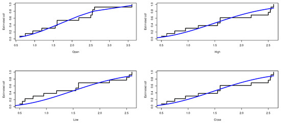
Figure 5. The estimated CDF of E-WD for the stock data.

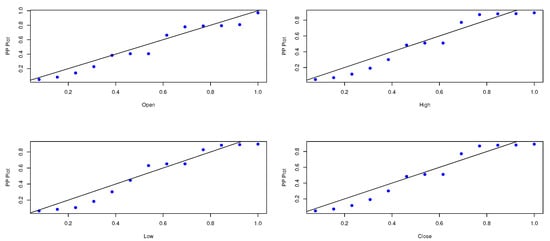
Figure 6. The PP plot of the E-WD.

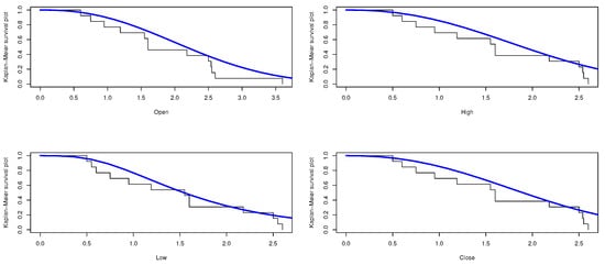
Figure 7. The Kaplan–Meier survival function of the E-WD.

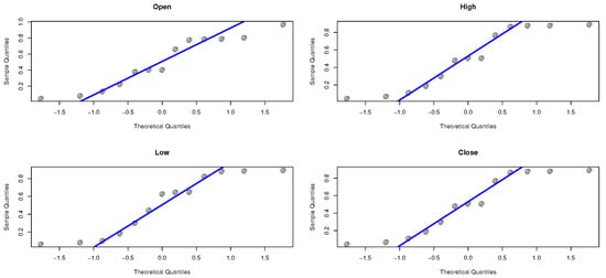
Figure 8. The Q-Q normality plot of the E-WD.

The goodness-of-fit results of the E-WD model are compared with some other models, including the Mudholkar exponintiated Weibull distribution [27] (MEWD), the generalized Weibull Modified Weibull distribution (GWMWD), the generalized Weibull-Rayleigh distribution (GWRD), the exponentiated distribution (EXP-CD). The CDF of the competing probability models are, respectively, given by

$$\begin{array}{c}\hfill F(y;\beta ,\iota ,\sigma )={\left(1-e^{-{\left(\iota y\right)}^{\sigma }}\right)}^{\beta },\end{array}$$

(57)

$$\begin{array}{c}\hfill F(y;\alpha ,\beta ,\omega ,\delta ,\nu )=1-e^{-\alpha {\left(\omega y+\delta y^{\nu }\right)}^{\beta }},\end{array}$$

(58)

$$\begin{array}{c}\hfill F(y;\tau ,\delta ,\mu )=1-e^{-\tau {\left(\mu y^2\right)}^{\delta }},\end{array}$$

(59)

and

$$\begin{array}{c}\hfill F(\tau ;\iota )=1-e^{-\iota \tau }.\end{array}$$

(60)

Table 8 compare the E-WD via some recognition criterion, such as The: Akaike information criterion (AIC), Bayesian information criterion (BIC), Hannan–Quinn information criterion (HQIC) and consistent Akaike information Criterion (CAIC). Table 9 compares the E-WD based on one-sample Kolmogorov-Smirnov test.

Table 8. Relative quality of the E-WD vs. competing models.

Model	AIC	CAIC	BIC	HQIC
E-WD	1278.283	1278.349	1290.007	1282.94
ZEWD	1301.776	1301.842	1313.500	1306.43
GWMW	1320.852	1320.918	1332.577	1325.51
Exp-D	1552.449	1552.459	1556.357	1554.01
GWRD	1307.332	1307.398	1319.056	1311.99

Table 9. One-sample Kolmogorov-Smirnov test for the E-WD and the competing models.

Model	KS	p-Value
E-WD	0.06257	0.112
OEWD	0.11489	0.0001
GWMW	0.10643	0.0004
EXP-D	0.31722	2.2e-16
GWRD	0.09666	0.0021

Table 9 compares the E-WD and the competing models with the Kolmogorov-Smirnov test for one sample. The results in Table 8 and Table 9 suggest that the E-WD model provides a better fit than other competing models and could be chosen as a suitable model for analyzing stock price data.

From the results in Table 8 and Table 9, it can be seen that the model E-WD could be selected as the best model among the fitted models because the proposed model has the lowest values for AIC, BIC, HQC, and CAIC and the highest values for Kolmogorov-Smirnov p-value.

10. Conclusions

Financial markets play basic role through financial operations, from issuing securities and offering them to investors to making them available for trading. The name of a share is derived from the concept of participation, because the share represents a certain part, a share or a piece of the capital of a listed company, and its owner is considered a shareholder of this company. Shares, for example—These are usually tradable through the trading methods prescribed in the money market regulations. In this study, we introduce a new three-parameter modification of the Weibull model, called the exponentiated Weibull distribution. We proofed that, the new model has many statistical advantages, the flexibility, the heavy-tailed behavior and the regular variation property were offered. We presented many of the important statistical functions including the quantile function, rth-moment, moment generating function, characteristic function, identifiability property, the information generating function, the Shannon entropy and the information energy have been derived in closed forms. The distribution parameters are estimated using the maximum likelihood approach and Bayesian estimation. The squared error loss function, the LINEX loss function, and the general entropy loss function are used for the Bayesian procedure. The simulation result shows that the Bayesian approach gives better estimates and specially Linex loss function with positive constant shows good performance. $95\%$ and $90\%$ interval estimate of each parameter and the corresponding width are obtained. The interval length increases as the confidence level increases as expected. We apply the new composite exponentiated Weibull distribution to the real stock exchange transaction data over four variables, the opening price, the high price, the low price, and the closing price. The goodness of fit results are compared with some other models. The comparisons are made using the Kolmogorov-Smirnov test for one sample and some recognition criterion, such as, the Akaike information criterion, Bayesian information criterion, Hannan-Quinn information criterion and consistent Akaike information criterion. The results indicate that the proposed model provides better fits than other competing models and could be chosen as an adequate model.

References

- Nadarajah, S.; Kot, S. The beta Gumbel distribution. Math. Probab. Eng. 2002, 10, 323–332. [Google Scholar] [CrossRef]
- Lingji, K.; Catl, L.; Sepanski, J.H. On the Properties of beta–gamma Distribution. J. Mod. Appl. Stat. Methods 2007, 6, 187–211. [Google Scholar]
- Akinsete, A.; Famoy, F.; Lee, C. The beta–pareto distribution. Statistics 2009, 42, 547–563. [Google Scholar] [CrossRef]
- Barreto-Souza, W.; Santos, A.H.S.; Cordeiro, G.M. The beta generalized exponential distribution. Statistics 2009, 42, 547–563. [Google Scholar] [CrossRef]
- Paranaiba, P.F.; Ortega, M.M.E.; Cordeiro, G.M.; Pescim, R.R. The beta Burr XII distribution with application to lifetime data. Comput. Stat. Data Anal. 2010, 55, 1118–1136. [Google Scholar] [CrossRef]
- Cordeiro, G.M.; Lemonte, A.J. The beta-half-Cauchy Distribution. J. Probab. Stat. 2011, 2011, 904705. [Google Scholar] [CrossRef]
- AL-Kadim, k.A.; Boshi, M.A. Exponential-Pareto Distribution. Math. Theory Model. 2013, 3, 135–146. [Google Scholar]
- Gupta, R.D.; Kundu, D. Generalized Exponential Distribution: Different method of estimation. J. Stat. Simul. 2000, 30, 315–338. [Google Scholar] [CrossRef]
- Nasiri, P. Estimation of Parameters of Generalized Exponential Distribution in Person of Outlier. 2006. Available online: http://www.m-hikari.com/ams/ams-2010/ams-45-48-2010/nasiriAMS45-48-2010.pdf (accessed on 13 March 2023).
- Martinez, E.Z.; Achcar, J.A.; Jacome, A.A.A.; Santos, J.S. Mixture and non-mixture cure fraction models based on the generalized modified Weibull distribution with an application to gastric cancer data. Comput. Methods Programs Biomed. 2013, 112, 343–355. [Google Scholar] [CrossRef]
- Carl, L.; Felix, F.; Olugbenga, O. Beta-Weibull Distribution: Some Properties and Applications to Censored Data. J. Mod. Appl. Stat. Methods 2007, 6, 173–186. [Google Scholar]
- Tahir, H.; Cordeiro, G.M.; Ayman, A.; Mansoor, M.; Zubair, M. A New Weibull–Pareto Distribution: Properties and Applications. Commun. Stat. Simul. Comput. 2011, 45, 3548–3567. [Google Scholar] [CrossRef]
- Emam, W. On Statistical Modeling Using a New Version of the Flexible Weibull Model: Bayesian, Maximum Likelihood Estimates, and Distributional Properties with Applications in the Actuarial and Engineering Fields. Symmetry 2023, 15, 560. [Google Scholar] [CrossRef]
- Emam, W.; Tashkandy, Y. The Arcsine Kumaraswamy-Generalized Family: MLE and Classical Estimates and Application. Symmetry 2022, 14, 2311. [Google Scholar] [CrossRef]
- Emam, W.; Tashkandy, Y. The Weibull Claim Model: Bivariate Extension, Bayesian, and Maximum Likelihood Estimations. Math. Probl. Eng. 2022, 2022, 8729529. [Google Scholar] [CrossRef]
- Emam, W.; Tashkandy, Y. Modeling the Amount of Carbon Dioxide Emissions Application: New Modified Alpha Power Weibull-X Family of Distributions. Symmetry 2023, 15, 366. [Google Scholar] [CrossRef]
- Emam, W.; Tashkandy, Y. A New Generalized Modified Weibull Model: Simulating and Modeling the Dynamics of the COVID-19 Pandemic in Saudi Arabia and Egypt. Math. Probl. Eng. 2022, 2022, 1947098. [Google Scholar] [CrossRef]
- Emam, W.; Tashkandy, Y. Khalil New Generalized Weibull Distribution Based on Ranked Samples: Estimation, Mathematical Properties, and Application to COVID-19 Data. Symmetry 2022, 14, 853. [Google Scholar] [CrossRef]
- Seneta, E. Karamata’s characterization theorem, feller and regular variation in probability theory. Publ. Inst. Math. 2002, 71, 79–89. [Google Scholar] [CrossRef]
- Bowley, A.L. Elements of Statistics, 4th ed.; Charles Scribner’s Sons: New York, NY, USA, 1920. [Google Scholar]
- Moors, J.J.A. The meaning of kurtosis: Darlington re-examined. Am. Stat. 1986, 40, 283–284. [Google Scholar]
- López-Ruiz, R.; Mancini, H.L.; Calbet, X. A statistical measure of complexity. Phys. Lett. 1995, 209, 321–326. [Google Scholar] [CrossRef]
- Golomb, S. The IGF of a probability distribution. IEEE Trans. Inf. Theory 1966, 12, 75–77. [Google Scholar] [CrossRef]
- Shannon, C. A Mathematical Theory of Communication. Bell Syst. Tech. J. 1948, 27, 379–423. [Google Scholar] [CrossRef]
- Cataron, A.; Andonie, R. How To Infer The Informational Energy from Small Datasets. In Proceedings of the 2012 13th International Conference on Optimization of Electrical and Electronic Equipment (OPTIM), Brasov, Romania, 24–26 May 2012; IEEE: Piscatawaj, NJ, USA, 2012; pp. 1065–1070. [Google Scholar]
- Kundu, D.; Joarder, A. Analysis of Type-II progressively hybrid censored data. Comput. Stat. Data Anal. 2006, 50, 2509–2528. [Google Scholar] [CrossRef]
- Mudholkar, G.S.; Srivastava, D.K. Exponentiated Weibull family for analyzing bathtub failure-rate data. IEEE Trans. Reliab. 1993, 42, 299–302. [Google Scholar] [CrossRef]
Disclaimer/Publisher’s Note: The statements, opinions and data contained in all publications are solely those of the individual author(s) and contributor(s) and not of MDPI and/or the editor(s). MDPI and/or the editor(s) disclaim responsibility for any injury to people or property resulting from any ideas, methods, instructions or products referred to in the content. |
© 2023 by the authors. Licensee MDPI, Basel, Switzerland. This article is an open access article distributed under the terms and conditions of the Creative Commons Attribution (CC BY) license (https://creativecommons.org/licenses/by/4.0/).