Abstract
The rock deformation and failure characteristics and mechanisms are very important for stability evaluation and hazard control in rock engineering. The process of rock deformation and failure is often accompanied by temperature changes. It is of great significance to study the characteristics and mechanism of temperature variation in rock under deformation and fracturing for a better understanding of rock failure and to obtain some probable precursor information for guiding the prediction of the mechanical behavior of rock. However, most of the studies are based on observations in the field and laboratory tests, while it is still required to develop an effective method for modeling and calculating the temperature variation of rock during the deformation and failure processes. In this paper, a particle flow modeling method based on energy analyses is proposed for simulating the temperature variation of rocks, considering four temperature effects, including the thermoelastic effect, friction effect, damping effect, and heat conduction effect. The four effects are analyzed, and the theoretical equations have been provided. On this basis, the numerical model is built and calibrated according to the laboratory uniaxial compressive experiment on a marble specimen, and a comparison study has been conducted between the laboratory and numerical experiment results. It is found that the numerical model can well simulate the average value and distribution of the temperature variation of rock specimens, so this method can be applied for studying the mechanism of temperature variation more comprehensively during the whole process of rock deformation and fracturing compared with the continuous modeling methods. With this method, it is shown that the temperature change has three different stages with different characteristics during the uniaxial compression experiments. In the different stages, the different effects play different roles in temperature variation, and stress distribution and crack propagation have obvious influences on the local distribution of temperature. Further investigations have also been conducted in a series of sensitive analyses on the influences of four factors, including the thermal conductivity, friction coefficient, thermal expansion coefficient, and particle size ratio. The results show that they have different influences on the thermal and mechanical behaviors of the rock specimens during the deformation and failure process, while the thermal expansion coefficient and the particle size ratio have more significant impacts than the other two factors. These findings increase our knowledge on the characteristics and mechanism of temperature variation in rock during the deformation and fracturing process, and the proposed modeling method can be used in more studies for deformation and fracturing analyses in rock experiments and engineering.
1. Introduction
Deformation and fracturing in the rock engineering may result in serious hazards, which may pose a great threat to the safety of engineering and even the lives of people. Therefore, it is necessary and important to strengthen the study of the mechanical behaviors and mechanisms of rock [1,2,3,4,5,6,7] as well as the early warning of rock failure [8,9]. The deformation and failure process of rocks is always associated with energy changes; consequently, temperature variations can be observed during the process. This provides us with a method to study the characteristics and mechanism of rock deformation and fracturing by monitoring the temperature variation [10]. These studies can be useful for a better understanding of the mechanisms of deformation and failure in rock engineering, such as rockbursts in tunnels and landslides of rocks. They may also be helpful for supplying some temperature precursor information for guiding prediction on the failure of rock [11,12,13].
Actually, the relation between rock failure and temperature variation has been applied to much research on seismic temperature anomalies. Through the study of earthquakes, it is found that rocks within a certain range of the earthquake areas are often accompanied by temperature anomalies during the seismogenic process and after the earthquake [14,15]. In order to explore the temperature anomalies of rocks, many experts and scholars have done a lot of research and analysis on the temperature anomalies by using different technologies. In the early stage, through the visual interpretation of the infrared radiation image monitored by the satellite [16], it was found that there were obvious infrared radiation anomalies near the earthquake area from days to months before the earthquake [17], and the anomaly area was mainly distributed along the fault near the epicenter [18]. Later, in order to analyze the variation characteristics of infrared radiation anomalies, the wavelet transform method [19], the background field removal method [20], the multi-channel method [21], and the power spectrum method [22] were proposed to further quantitatively analyze the image, which improved the ability of using infrared radiation images to analyze infrared radiation anomalies before and after earthquake events. In addition to the use of satellite data, the temperature observation of bedrock at different depths was also observed by means of borehole temperature measurement [23,24,25]. It is recognized that there are not only heating but also cooling areas before the earthquake, and the precursor information has the characteristics of near field, structural correlation, and sensitivity to stress changes. The researchers used different technical means and data processing methods to study the temperature anomalies before and after the earthquake. During the earthquake preparation process, they realized that there were temperature anomalies in the rocks in the earthquake area and summarized the spatial and temporal characteristics of the temperature anomalies. However, because technologies such as satellite monitoring, borehole temperature measurement, and so on are usually affected to varying degrees by factors such as complex terrain, changeable climate, vegetation cover, stress disturbance, and so on, the accuracy of temperature data is also affected. In addition, because of the different geological structures, in-situ stresses, and formation lithology in various regions, it is difficult to systematically study the characteristics and mechanism of temperature changes. Consequently, the relation between temperature variation and the deformation and fracturing of rock during the earthquake process is still not clearly known, especially the mechanism, which still needs to be investigated.
Because more accurate experimental conditions can be applied and the temperature of rock can be measured more precisely in the laboratory, researchers have conducted a series of laboratory experiments to study the temperature effect of rock during the deformation and fracturing processes. Uniaxial compression [26], multiaxial compression and shear tests [27,28] on rocks with different lithologies [29] proved that the infrared radiation of rocks would change under different stress conditions. In order to accurately grasp the characteristics of infrared radiation evolution, a variety of methods were used to process the infrared radiation data [30]. In addition to using the average temperature [31], a variety of parameters were also introduced to characterize the temperature evolution process and predict rock failure, for example, the temperature standard deviation index [32], characteristic roughness, entropy, and variance [33], continuous minimum infrared image temperature variance [34], instantaneous variance of infrared image sequence [35], infrared radiation b value [36], temperature concentration coefficient [37], and temperature variation coefficient [38]. On this basis, the influencing factors of infrared radiation are further studied. It is considered that the temperature change is related to the type of fracture [27], water in rock [39], volume strain [40], stress [41], and heat conduction effect [42]. In these studies, the temperature evolution can be captured and analyzed in conjunction with the stress-strain curves and macro-fractures; however, these studies are always based on the observation of the temperature change of the rock, with no detailed information including the stress and strain distribution, the micro-crack initiation and propagation, etc., known. Consequently, the mechanism of the temperature variation during the rock deformation and fracturing process is still not clear.
In recent years, the development of numerical modeling has provided us with a new way of analyzing mechanical and thermal behaviors. Wang et al. [43] carried out a series of numerical calculations on metal materials with a finite element numerical calculation of metal materials. In addition, the results show that elastic tension causes a temperature drop, while elastic compression causes the temperature to rise in the elastic stage. However, if the material is in the elastic-plastic deformation range, plastic tension, elastic compression, and plastic compression lead to an increase in the material temperature, while elastic tension leads to a decrease in the material temperature. However, numerical methods based on continuous modeling methods, such as the finite element method and boundary element method, are difficult for studying the dominant mechanisms of rock failure processes related to micro-crack initiation, propagation, and coalescence [44]. The discrete element method can simulate different arrangements of rock grains, the initiation, propagation, and coalescence of micro-cracks, and obtain the evolution of stress and strain distribution during the process, so it provides a better way for understanding the characteristics and mechanism with more detailed information. Nonetheless, this type of modeling is always adopted to study the influence of temperature on the mechanical behaviors of rock [45,46], while it is still required to develop an effective method to analyze the temperature variation during the deformation and fracturing process based on discrete element modeling. Liu et al. [47] applied the discrete element method to study the thermal effect in the process of rock failure, considering three kinds of heat, i.e., viscous heat, frictional heat, and breaking heat. In fact, it is believed that the thermoelastic effect [48] should not be ignored. In addition, the heat conduction effect between the rock particles should also be considered in the modeling.
Inspired by the above-mentioned research developments and problems, this paper intends to propose a particle flow modeling method to simulate and analyze the temperature variation of rock during deformation and fracturing based on energy analyses, considering four factors affecting temperature, including the thermoelastic effect, friction effect, damping effect, and heat conduction effect. A particle flow model will be built and calibrated based on laboratory experiments, and further characteristics and mechanism studies will be conducted consistently, considering different influencing factors based on the particle flow modeling method proposed in this paper. This proposed method can be applied to different types of rock under different stress conditions to investigate the characteristics and mechanism of temperature variation during the rock deformation and fracturing process, which will be very helpful for guiding the stability analyses and hazard control in rock engineering.
2. Temperature Variation in Particle Flow Modeling Based on Energy Analyses
The temperature calculation in the particle flow model should be based on the energy change. It is required to monitor the energy generation and transfer for each particle during the deformation and fracturing processes of a rock model. The heat change will be affected by the energy contributed by the thermoelastic effect, friction effect, and damping effect. In the meantime, the heat conduction effect should also be considered for energy transfer. It is assumed that the above-mentioned energy will all be converted to heat, and thereafter the temperature can be computed based on the heat. The temperature change of each particle can be calculated as follows:
where ΔT is the temperature change of each particle, ΔTt is the temperature change caused by the thermoelastic effect, ΔTf is the temperature change caused by the friction effect, ΔTd is the temperature change caused by the damping effect, ΔTh is the temperature change caused by the heat conduction effect.
The application of the thermoelastic effect, friction effect, damping effect, and heat conduction effect in the model is discussed below.
2.1. Thermoelastic Effect
The thermoelastic effect indicates the physical behavior that a small change in temperature will occur when the material is subjected to an elastic strain change induced by loading or unloading, and the thermoelastic effect is always described with Equation (2) [49]:
where T0 is the initial temperature, α is the coefficient of thermal expansion, ρ is the density, Cp is the specific heat capacity at constant pressure, and Δσkk is the variation of the principal stress sum.
Although the real rock grains have micro-structures, a simplified and conceptual model is used in the particle flow modeling, where the particle is assumed to be intact and rigid, and the elastic deformation is simulated with the overlap between particles [50]. Therefore, the thermoelastic effect should be specially considered for the particles to calculate the temperature change in the rock grains.
According to the stress analysis in elastic mechanics, the principal stresses (σ1, σ2) under plane stress state have the following relation with the stress components (σx, σy):
Consequently, in PFC2D modeling, the temperature change ΔTt of each particle induced by the thermoelastic effect between time steps t and t + 1 can be expressed as:
During the calculation, it is assumed that the thermal expansion coefficient α, particle density ρ, and specific heat capacity Cp are constants, as the changes in temperature and pressure cannot have considerable influences on these parameters during the testing process.
2.2. Friction Effect
When there is a relative displacement between two contacted particles, the friction will take effect, and the friction energy will contribute to the heat and hence lead to a change in temperature.
In particle flow modeling, friction energy Eμ is defined as a kind of cumulative energy, updated in the program as Equation (5) [51]:
where (Fsl)0 is the linear shear force at the beginning of the time step, (Fsl)1 is the linear shear force at the end of the time step, and Δδsμ is the relative sliding shear displacement.
The friction energy in the loading process is thought to be completely converted into heat Qf:
Thereafter, the temperature change ΔTf caused by the friction effect can be obtained according to the heat calculation formula:
where Cp is the specific heat capacity at constant pressure and m is the mass of the particle. It should be noted that the heat Qf is assumed to be equally distributed between the two contacted particles.
2.3. Damping Effect
In the particle flow modeling, the damping is required to dissipate the kinetic energy associated with the seismic waves [47], so the dissipated kinetic energy will contribute to the production of heat. The damping can be considered at either the normal or shear directions on the contact between two particles, with the normal or shear critical damping ratio. The definition of the damping model is introduced in [51] with more detailed descriptions and equations.
Consequently, similar to the friction energy, the damping energy Ed on contact can also work on the particles to cause a temperature rise. In particle flow modeling, damping energy is also defined as a type of cumulative energy, and it is updated as Equation (8) [51]:
where Fd is the damping force, is the relative velocity, and Δt is the time step.
It is assumed that the work done by the damping on the particles is all converted into heat Qd:
Thereafter, the temperature change ΔTd caused by the damping effect can be obtained according to the heat calculation formula:
where Cp is the specific heat capacity at constant pressure and m is the mass of the particle. It should be noted that the heat Qd is assumed to be distributed equally between the two contacted particles.
2.4. Heat Conduction Effect
Heat conduction will occur when there is a temperature difference between the contacted particles; therefore, the heat conduction effect cannot be ignored when computing a change in temperature. The heat conduction effect does not cause a change in total heat, but only transfers heat from one particle to another.
In the particle flow modeling, the thermal material is represented as a network of heat reservoirs (associated with each particle) and thermal contacts (associated with mechanical contacts). Heat flow occurs by means of the conduction in the active thermal contacts connecting reservoirs. Each particle represents a heat reservoir, and each reservoir has a series of properties including temperature, mass, volume, specific heat capacity, and coefficient of linear thermal expansion. The thermal contact connects two heat sources, and the heat flow occurs only through the thermal contact [51].
Although temperature change may occur due to strain change, it should be noted that this temperature change can be assumed to be negligible for quasi-static mechanical problems. The heat conduction effect can be described with the heat conduction equation for a continuous medium [51]:
where qi is the heat flux vector, xi is the location, qv is the volume heat source intensity or power density, ρ is the mass density, Cv is the specific heat capacity at constant volume, T is the temperature, and t is the time.
Note that for nearly all solids and liquids, the specific heat capacities at constant pressure and at constant volume are essentially equal. Consequently, Cp and Cv can be used interchangeably [51].
3. Comparison Study on Experimental and Numerical Results
3.1. Laboratory Experiment
The uniaxial compression experimental study on marble specimens [52] is used here for the calibration of the numerical model and the comparison analyses. In the laboratory experiment, the marble specimen has the size of 50 mm × 50 mm × 100 mm, and the main minerals are dolomite (96.98%) and calcite (3.02%). The uniaxial compression tests were conducted using an electric servo-hydraulic material testing machine (INSTRON 1346) with a constant strain rate of 4 × 10⁻⁵/s. Complete stress-strain curve has been obtained (Figure 1), and it is shown that the uniaxial compressive strength (UCS) is 124 MPa (σc = 124 Mpa) and the elastic modulus is 23 GPa. During the experimental process, an uncooled infrared thermographic camera (SC7000 FLIR) with the temperature sensitivity of 0.01 °C was used to monitor the variation of rock temperature by capturing infrared radiation (IRR) images at a 100 Hz frame rate (Figure 2). The images show that the temperature accumulates on the surface of the specimen during the pre-peak stage, while the macro fractures lead to a more heterogeneously distributed temperature in the post-peak stage.
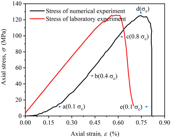
Figure 1.
A complete stress-strain curve of the marble specimen under uniaxial compression experiment [based on [52]].
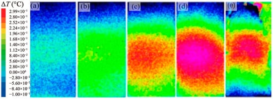
Figure 2.
Infrared radiation image of a marble specimen subjected to uniaxial compression experiment at different stress levels (a) 0.1 σc; (b) 0.4 σc; (c) 0.8 σc; (d) σc; (e) 0.1 σc [52].
3.2. Numerical Modeling
In this paper, a 100 mm × 50 mm rectangular rock model is built with PFC2D. The mechanical model should be established first; thereafter, the thermodynamic model would be built on the basis of the mechanical model. When the model is running, applying axial loading leads to a change in stress distribution in the model. The stress change will induce a change in temperature distribution caused by the thermoelastic effect, friction effect, damping effect, and heat conduction effect as described in Section 2. In the meantime, the change in temperature will also have an influence on the stress distribution in the model. The calculation process of this thermo-mechanical coupling model is demonstrated in Figure 3.
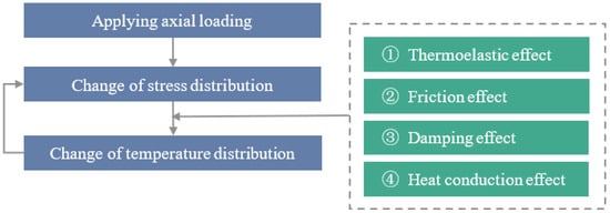
Figure 3.
Calculation process of the thermo-mechanical coupling model.
A flowchart for the work process in this study is shown in Figure 4. This process includes several main steps, as follows:
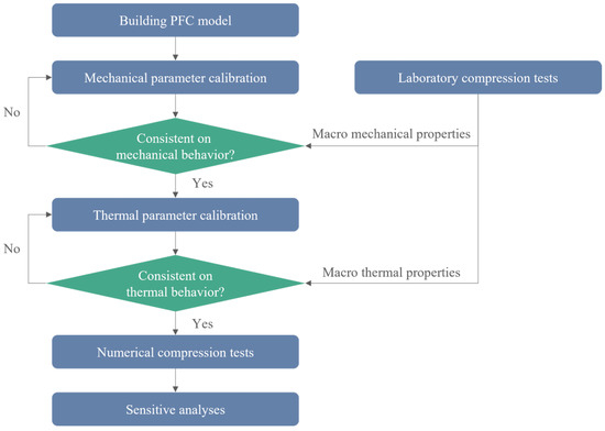
Figure 4.
Flowchart for the work process.
- (1)
- Building the particle flow model and calibrating the mechanical parameters according to the mechanical behaviors (macro mechanical properties) in the laboratory compression test results;
- (2)
- Calibrating the thermal parameters according to the temperature variations (macro thermal properties) in the laboratory compression test results;
- (3)
- Conducting a series of numerical experiments and sensitive analyses considering different factors for the further mechanism studies.
According to the flowchart in Figure 4, the mechanical model is built first with a linear, parallel bond model between particles. The calibrated parameters of the model are listed in Table 1. The numerical uniaxial compression experiment shows that this model has similar stress-strain behavior to the laboratory experimental result (Figure 1). The calculated UCS is 125 MPa, and the elastic modulus is 22.8 GPa, which are also very close to the laboratory experiment results.

Table 1.
Microparameters of the contact bond model and parallel bond model.
The thermodynamic model is built by implanting the thermodynamic calculation scheme into the above-mentioned mechanical model [53], and three steps are required as follows:
- (1)
- Giving the basic thermal parameters. The basic thermal parameters are given as shown in Table 2.
Table 2. Thermal parameters of the granite thermodynamic model [based on [54]].
- (2)
- Distributing the thermal contact model. The thermal pipe contact model is distributed between particles and has two modifiable parameters: the thermal expansion coefficient, α, and the thermal resistance, η. The thermal resistance is calculated according to the thermal conductivity [51]:where k is the thermal conductivity, n is the porosity, V is the volume of particles, Nb is the number of particles, Np is the activated heat pipe, and l(p) is the heat pipe length related to particles.
- (3)
- Setting the initial and boundary conditions. An adiabatic environment is created by setting a null thermal contact model between the walls and the particles. The null thermal contact model does not participate in the conduction of heat, so there is no heat exchange between the particles and the walls. The initial temperature is set at 26.85 °C (300 K).
3.3. Comparison Study
The model was loaded at a constant strain rate of 1/s. During the loading process, the average temperature change ΔTave was recorded as Equation (13):
where i is the number of particles and Ti is the temperature of the i-th particle.
The change in average temperature change ΔTave exhibited in Figure 5 is associated with increasing axial strain and stress, respectively. According to Figure 5a, for both the laboratory and numerical experiments, ΔTave increases gradually with the increasing strain to a maximum value of about 0.28 °C and then goes down quickly. It should be noted that there is a small gap between the two curves because the compaction-induced strain at the initial loading stage cannot be shown in the particle flow model with densely packed balls [55]. Figure 5b shows that the general trend of ΔTave in the numerical model has quite a good agreement with that in the laboratory experiment.
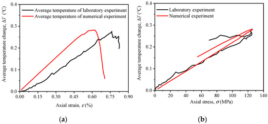
Figure 5.
Changes in average temperature ΔTave are associated with increasing axial strain (a) and axial stress (b) in the laboratory experiment and the numerical experiment.
The temperature distribution image is shown in Figure 6. The temperature distribution on the rock surface is more uniform in the early stages of loading, and the discreteness of the temperature distribution increases after the model is broken.
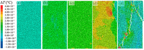
Figure 6.
Particle temperature diagram of the numerical experiment at different stress levels (a) 0.1 σc; (b) 0.4 σc; (c) 0.8 σc; (d) σc; (e) 0.1 σc.
In order to have a better understanding of the characteristics and mechanism of temperature distribution, the temperature images (Figure 6) as well as the force chains (Figure 7) and crack propagation (Figure 8) of the specimen are obtained at different stress levels (0.1 σc, 0.4 σc, 0.8 σc, σc, 0.1 σc) during the numerical experiment. Compared with Figure 2 and Figure 6, it is observed that the temperature increases with the axial stress increasing to the peak stress σc, and this general trend is similar to the phenomenon of the laboratory experiment shown in Figure 2. Meanwhile, the temperature variation range of the rock specimen is about −0.1 °C–0.3 °C, and the temperature variation range of the model is about −0.1 °C–0.5 °C. The variation ranges in the laboratory experiment and the numerical experiment are very close.
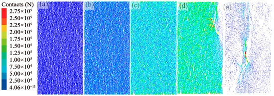
Figure 7.
Force chain diagram of a numerical experiment at different stress levels (a) 0.1 σc; (b) 0.4 σc; (c) 0.8 σc; (d) σc; (e) 0.1 σc.
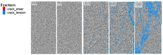
Figure 8.
Crack propagation diagram of the numerical experiment at different stress levels (a) 0.1 σc; (b) 0.4 σc; (c) 0.8 σc; (d) σc; (e) 0.1 σc.
However, there are also several differences between the laboratory and numerical experiment results, as follows:
- (1)
- The temperature rise covers most of the area in the numerical model (Figure 6d), while it is much more significant in the middle part than the two ends of the rock specimen (Figure 2d). This difference is due to the adiabatic environment applied in the numerical model. There is no heat exchange between the specimen and the sidewalls connected to the two ends in the numerical model, but the heat will flow to the steel loading platen in the laboratory experiment, so the temperature in the rock specimen is quite lower than that at both ends. This is also the reason why the temperature variation range in the numerical model (−0.1 °C–0.5 °C) is slightly larger than that in the rock specimen (−0.1 °C–0.3 °C).
- (2)
- The temperature variation is more heterogeneous in the numerical model (Figure 6d) than that in the rock specimen (Figure 2d) in the laboratory experiment. At the initial stage of loading, the temperature is low and evenly distributed for both the numerical model and rock specimen. As the loading continues, the temperature increases and decreases are more clearly observed in different areas of the numerical model. This can be better understood when compared with the distribution evolution of force chains (Figure 7) and crack propagation (Figure 8). The larger contact force means higher concentration, which will lead to a localized temperature rise. Crack propagation can induce some stress drop and, as a result, some localized temperature reduction. This result is more obvious in the 2D numerical model than in the rock specimen because the stress concentration may occur inside the specimen and crack propagation may not go through it [52]. Another possible reason is that the heat exchange between the rock and the steel loading platen or the air environment is helpful for a more homogeneously distributed temperature. In the post-peak stage, macrofractures can be observed in both the rock specimen (Figure 2e) and numerical model (Figure 6e), and the temperature distributions are both heterogeneous, showing the temperature variation influenced by the fractures.
According to the comparison between the numerical and laboratory experiments, it can be seen that the temperature variation can be generally modeled by the particle flow modeling method provided by this research. Although there are some differences owing to the different test environments in the numerical and physical conditions, the general variation trends of the temperature value and distribution are quite similar. Furthermore, the particle flow model can be used to carry out a series of consistent studies on the mechanism, considering different factors. This will be discussed in the next section.
4. Discussion
4.1. Characteristics of Temperature Change and Mechanism Analyses
In order to know more about the mechanism of the temperature change, ΔTave is studied in combination with the temperature change contributed by the thermoelastic effect, friction effect, and damping effect during the loading process. It should be noted that the heat conduction effect is not analyzed here because it does not produce or release heat but only transfers heat between different particles. The microcrack number is also compared here to observe its influence on the temperature change. The curves are shown in Figure 9. According to the characteristics of temperature change, the whole process is divided into three stages: stage a, stage b, and stage c.
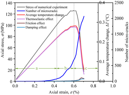
Figure 9.
Axial stress, number of micro-cracks, and average temperature change with the axial strain during the numerical experiment under uniaxial compression.
Stage a: The average temperature change ΔTave increases linearly with increasing axial strain. The axial stress also increases linearly in this stage. The temperature contributed by the thermoelastic effect grows significantly while the curves for the other effects remain about zero, indicating that the temperature rise is almost entirely caused by the thermoelastic effect. The number of microcracks is almost zero, meaning that no obvious crack propagation occurs at this stage.
Stage b: The average temperature change ΔTave continues to grow at a decreasing growth rate until it reaches the peak value. The thermoelastic effect still plays a dominant role in the temperature sources, and the growing trend is very similar to that of ΔTave. In this stage, the friction effect begins to produce some temperature and keeps increasing slowly, and the number of microcracks begins to increase obviously, which leads to a lot of friction.
Stage c: The average temperature change ΔTave decreases significantly, accompanied by a significant decrease in axial stress. The thermoelastic effect is also obviously weakened, while the friction effect and damping effect are obviously enhanced. The number of microcracks continues to increase rapidly, and the friction effect produces more heat while the local stress drop makes the temperature decrease with the rapid crack propagation.
The stress and temperature effects at different stages are very different, owing to the different internal stress distribution and crack development at different stages. The internal meso-mechanism needs to be explored more thoroughly.
The model contains many parameters, and different parameters have different effects on the model. Several important parameters, including the thermal conductivity, friction coefficient, thermal expansion coefficient, and particle size ratio, are considered in the following studies to understand their influences on the thermal and mechanical behaviors of the model.
4.2. Influence of Thermal Conductivity
According to Equation (12), it can be seen that the thermal conductivity affects the thermal resistance value in the model. The smaller the thermal conductivity, the greater the thermal resistance. The thermal conductivity is set to be 0.68 W/(m/K), 1.68 W/(m/K), 2.68 W/(m/K), 3.68 W/(m/K), and 4.68 W/(m/K) in five different numerical tests, while keeping the other parameters constant. Figure 10a shows that the average temperature changes of the five experiments before the peak almost coincide. Although there is a slight fluctuation after the peak, the difference is not obvious. As shown in Figure 10b, the peak strength is also relatively stable. It can be concluded that the thermal conductivity in a certain range has little effect on the average temperature and peak strength of the model.

Figure 10.
Effect of different thermal conductivity on average temperature change (a); peak stress and the maximum value of average temperature change (b).
This result proves that the heat conduction effect does not produce heat but rather determines the amount of heat transferring between particles, so the average temperature change of the model is almost independent of the thermal conductivity.
4.3. Influence of Friction Coefficient
The friction coefficient is set to be 0.01, 0.1, 0.5, 0.8, and 1 in five different numerical tests, and its influences on the average temperature change and peak stress are shown in Figure 11. Before the peak, the growing rate of average temperature change ΔTave increases with the increase in friction coefficient. The peak values of ΔTave and UCS both have a general trend of slight growth with the increasing friction coefficient, although there are some small fluctuations. On one hand, the higher friction coefficient causes a higher temperature rise induced by the friction effect. On the other hand, the higher friction coefficient leads to a higher UCS, and then the temperature will also increase under higher axial stress. Above all, the increasing friction coefficient does lead to an increase in average temperature, although this influence is not very significant. After the peak, the average temperature change ΔTave decreases rapidly with the increasing axial strain.
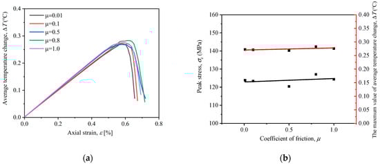
Figure 11.
Effect of different friction coefficients on average temperature change (a); peak stress and the maximum value of average temperature change (b).
4.4. Influence of the Thermal Expansion Coefficient
The thermal expansion coefficient has a key influence on the thermal properties of the model. The thermal expansion coefficient of the particles is set to be a series of values ranging from 1.35 × 10⁻⁷/K to 1.035 × 10⁻⁵/K. As shown in Figure 12, both the growing rate and peak value of the average temperature change (ΔTave) increase with the increase of the thermal expansion coefficient. This result also shows that the thermoelastic effect has a significant influence on the temperature change.
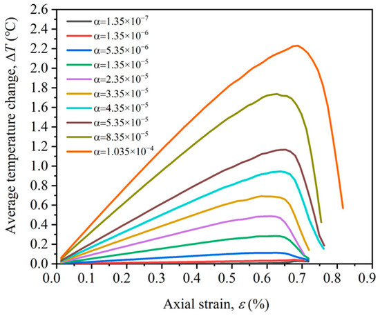
Figure 12.
Effect of different coefficients of thermal expansion on average temperature change.
4.5. Influence of Particle Size Ratio
Particle size ratio: the ratio of the maximum particle size to the minimum particle size in the model. Rocks in nature have different structures, even if the rocks of the same lithology have different particle sizes, so it is necessary to study the effect of particle size on the thermodynamic properties of the model. The average particle size in different models remains constant, while the particle size ratio is changed to be 1.5, 2.5, 3.5, 4.5, and 5, respectively. As shown in Figure 13b, the maximum peak stress is about 150 MPa and the minimum peak stress is about 120 MPa; the peak strength shows a trend of decreasing first and then increasing. The particle size ratio has a significant effect on the peak strength. Similarly, the average temperature change also decreases first and then increases (see Figure 13a). It can also be concluded that the mechanical properties of the model affect the thermal properties.
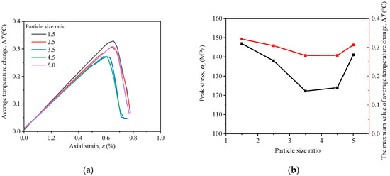
Figure 13.
Effects of different particle size ratios on average temperature change (a), peak stress and the maximum value of average temperature change (b).
In summary, different parameters have different influences on the thermal and mechanical properties of the model. More consistent and comprehensive research should be carried out in the future to consider more influencing factors, and a better understanding will be obtained by comparing more laboratory experiments on different rock types.
5. Conclusions
In this paper, a particle flow modeling method based on energy analyses is proposed, aiming at solving the problems of modeling and analyzing the characteristics and mechanism of temperature variation of rock during deformation and fracturing. The numerical model has been built and calibrated, and a comparison study has been conducted between the laboratory and numerical experiment results. On this basis, further discussions have been held for a better understanding of the mechanism, considering different influencing factors. There are several conclusions that can be drawn, as follows:
- (1)
- The proposed particle flow modeling method considers four different effects, including the thermoelastic effect, friction effect, damping effect, and heat conduction effect. The theoretical equations for calculating the temperature variation caused by each of the four effects have been provided, and this supplies a strong foundation for effective numerical modeling and further mechanism analyses.
- (2)
- The numerical model can well simulate the average value and distribution of the temperature variation of rock specimens under uniaxial compression, although there are several differences in the temperature distribution between the laboratory and numerical experiment results, owing to different heat exchange conditions between the physical and numerical environments. It is shown that this proposed method provides a better way for understanding the mechanism of temperature variation during the rock deformation and fracturing process, as this model can give more detailed information, including the evolution of stress and strain distribution, micro-crack initiation, propagation, coalescence, etc. during the process. This detailed information can provide a deeper insight into the characteristics and mechanisms compared with the field and laboratory observations and the continuous modeling method.
- (3)
- Based on this proposed modeling method, it is found that the temperature change has three different stages with different characteristics during the uniaxial compression. In the different stages, the different effects play different roles in temperature change, and the thermoelastic effect has the greatest impact on temperature compared to the other three effects. In addition, the stress distribution and crack propagation have obvious influences on the local distribution of temperature.
- (4)
- Four parameters, including the thermal conductivity, friction coefficient, thermal expansion coefficient, and particle size ratio, have been considered and found to have different influences on the thermal and mechanical behaviors of the rock specimen under uniaxial compression. It is shown that the thermal expansion coefficient and the particle size ratio have more significant impacts on temperature variation than the other two factors. These findings increase our knowledge on the mechanism of temperature variation during rock deformation and fracturing processes.
Above all, the proposed modeling method provides a new way to analyze the characteristics and mechanism of rock temperature variation during deformation and fracturing with more detailed information such as stress and strain distributions as well as micro-cracks. Although this study only considers intact rocks under uniaxial compression, in future research, more rock types with different structures under different stress conditions will be analyzed, and further mechanisms should be studied more consistently and comprehensively in combination with the laboratory experiments and the numerical studies based on the particle flow modeling method proposed in this paper.
This proposed method can be applied for modeling laboratory experiments and field engineering, and it will be helpful for knowing more about the mechanism of rock failure in engineering and earthquakes. It may also help us obtain some probable precursor information for guiding the prediction and early warning of the hazards in rock engineering and earthquakes.
Author Contributions
Conceptualization, C.C.; methodology, C.C.; software, X.J., G.W. and L.H.; validation, X.J.; formal analysis, C.C. and X.J.; investigation, C.C. and X.J.; resources, C.C. and X.J.; data curation, X.J. and Y.S.; writing—original draft preparation, X.J.; writing—review and editing, C.C.; supervision, C.C.; funding acquisition, C.C. All authors have read and agreed to the published version of the manuscript.
Funding
This research is funded by the Project for compilation and revision of highway engineering industry standards, Ministry of Transport of China (JTG-202059), and National Natural Science Foundation of China (No. 51991362).
Institutional Review Board Statement
Not applicable.
Informed Consent Statement
Not applicable.
Data Availability Statement
The data presented in this study are available on request from the corresponding author.
Acknowledgments
Z. Wang is appreciated here for his help and support in the software.
Conflicts of Interest
The authors declare no conflict of interest.
References
- Vipulanandan, C.; Mohammed, A. Hydraulic Fracturing Fluid Modified with Nanosilica Proppant and Salt Water for Shale Rocks; American Association of Drilling Engineers: Houston, TX, USA, 2015. [Google Scholar]
- Vipulanandan, C.; Mohammed, A.; Mahmood, W. Characterizing Rock Properties and Verifying Failure Parameters Using Data Analytics with Vipulanandan Failure and Correlation Models; American Rock Mechanics Association: Alexandria, VA, USA, 2021; p. 1614. [Google Scholar]
- Li, Y.; Hishamuddin, F.N.S.; Mohammed, A.S.; Armaghani, D.J.; Ulrikh, D.V.; Dehghanbanadaki, A.; Azizi, A. The Effects of Rock Index Tests on Prediction of Tensile Strength of Granitic Samples: A Neuro-Fuzzy Intelligent System. Sustainability 2021, 13, 10541. [Google Scholar] [CrossRef]
- Hasanipanah, M.; Jamei, M.; Mohammed, A.S.; Amar, M.N.; Hocine, O.; Khedher, K.M. Intelligent prediction of rock mass deformation modulus through three optimized cascaded forward neural network models. Earth Sci. Inform. 2022, 15, 1659–1669. [Google Scholar] [CrossRef]
- Xie, S.; Lin, H.; Chen, F.; Wang, Y.; Cao, R.; Li, J. Statistical Damage Shear Constitutive Model of Rock Joints Under Seepage Pressure. Front. Earth Sci. 2020, 8, 232. [Google Scholar] [CrossRef]
- Xie, S.; Han, Z.; Hu, H.; Lin, H. Application of a novel constitutive model to evaluate the shear deformation of discontinuity. Eng. Geol. 2022, 304, 106693. [Google Scholar] [CrossRef]
- Xie, S.; Lin, H.; Duan, H. A novel criterion for yield shear displacement of rock discontinuities based on renormalization group theory. Eng. Geol. 2023, 314, 107008. [Google Scholar] [CrossRef]
- Li, Z.; Xu, R. An early-warning method for rock failure based on Hurst exponent in acoustic emission/microseismic activity monitoring. Bull. Eng. Geol. Environ. 2021, 80, 7791–7805. [Google Scholar] [CrossRef]
- Di, Y.; Wang, E. Rock Burst Precursor Electromagnetic Radiation Signal Recognition Method and Early Warning Application Based on Recurrent Neural Networks. Rock Mech. Rock Eng. 2021, 54, 1449–1461. [Google Scholar] [CrossRef]
- Yao, X.; Teng, Y.; Xie, T. Thermal infrared brightness temperature anomaly evolution associated with the Songyuan Ms5.7 earthquake on May 28, 2018. Acta Sieismol. Sinica 2019, 41, 343–353. [Google Scholar]
- Sun, X.; Xu, H.; He, M.; Zhang, F. Experimental investigation of the occurrence of rockburst in a rock specimen through infrared thermography and acoustic emission. Int. J. Rock Mech. Min. Sci. 2017, 93, 250–259. [Google Scholar] [CrossRef]
- Liu, X.; Liang, Z.; Zhang, Y.; Liang, P.; Tian, B. Experimental study on the monitoring of rockburst in tunnels under dry and saturated conditions using AE and infrared monitoring. Tunn. Undergr. Space Technol. 2018, 82, 517–528. [Google Scholar] [CrossRef]
- Cao, K.; Ma, L.; Wu, Y.; Spearing, A.S.; Khan, N.M.; Hussain, S.; Rehman, F.U. Statistical damage model for dry and saturated rock under uniaxial loading based on infrared radiation for possible stress prediction. Eng. Fract. Mech. 2022, 260, 108134. [Google Scholar] [CrossRef]
- Zhang, L.; Guo, X.; Zhang, X.; Tu, H. Anomaly of thermal infrared brightness temperature and basin effect before Jiuzhaigou MS7.0 earthquake in 2017. Acta Seismol. Sin. 2018, 40, 797–808. [Google Scholar]
- Jing, F.; Zhang, L.; Singh, R.P. Pronounced Changes in Thermal Signals Associated with the Madoi (China) M 7.3 Earthquake from Passive Microwave and Infrared Satellite Data. Remote Sens. 2022, 14, 2539. [Google Scholar] [CrossRef]
- Wu, L.; Qin, K.; Liu, S. progress in analysis to remote sensed thermal abnormity with fault activity and seismogenic process. Acta Geod. Et Cartogr. Sin. 2017, 46, 1470–1481. [Google Scholar]
- Saraf, A.K.; Rawat, V.; Das, J.; Zia, M.; Sharma, K. Satellite detection of thermal precursors of Yamnotri, Ravar and Dalbandin earthquakes. Nat. Hazards 2012, 61, 861–872. [Google Scholar] [CrossRef]
- Lu, X.; Meng, Q.; Gu, X.; Zhang, X.; Xie, T.; Geng, F. Thermal infrared anomalies associated with multi-year earthquakes in the Tibet region based on China’s FY-2E satellite data. Adv. Space Res. 2016, 58, 989–1001. [Google Scholar] [CrossRef]
- Xie, T.; Kang, C.; Ma, W. Thermal infrared brightness temperature anomalies associated with the Yushu (China) Ms = 7.1 earthquake on 14 April 2010. Nat. Hazards Earth Syst. Sci. 2013, 13, 1105–1111. [Google Scholar] [CrossRef]
- Yang, X.; Zhang, T.; Lu, Q.; Long, F.; Liang, M.; Wu, W.; Gong, Y.; Wei, J.; Wu, J. Variation of Thermal Infrared Brightness Temperature Anomalies in the Madoi Earthquake and Associated Earthquakes in the Qinghai-Tibetan Plateau (China). Front. Earth Sci. 2022, 10, 332. [Google Scholar] [CrossRef]
- Yue, Y.; Chen, F.; Chen, G. Statistical and Comparative Analysis of Multi-Channel Infrared Anomalies before Earthquakes in China and the Surrounding Area. Appl. Sci. 2022, 12, 7958. [Google Scholar] [CrossRef]
- Zhong, M.; Shan, X.; Zhang, X.; Qu, C.; Guo, X.; Jiao, Z. Thermal Infrared and Ionospheric Anomalies of the 2017 Mw6.5 Jiuzhaigou Earthquake. Remote Sens. 2020, 12, 2843. [Google Scholar] [CrossRef]
- Yang, X.; Liu, W.; Yeh, E.C. Analysis on the mechanisms of cosemic temperature negative anomaly in fault zone. Chinese J. Geophys. 2020, 63, 1422–1430. (In Chinese) [Google Scholar]
- Chen, S.; Song, C.; Yan, W. Change in bedrock temperature before and after Jiashi MS6.4 earthquake in Xinjiang on January 19, 2020. Seismol. Geol. 2021, 43, 447–458. [Google Scholar]
- Chen, S.; Ma, J.; Liu, P.; Liu, L.; Jiang, J. Exploration on the relationship between surface thermal infrared radiation and borehole strain. Prog. Nat. Sci. 2008, 18, 145–153. [Google Scholar]
- Chen, G.; Li, Y.; Chen, Y.; Ma, J.; Wu, Z. Thermal-acoustic sensitivity analysis of fractured rock with different lithologies. Chin. J. Rock Mech. Eng. 2022, 41, 1945–1957. [Google Scholar]
- Liu, S.; Wu, L.; Wu, Y. Infrared radiation of rock at failure. Int. J. Rock Mech. Min. Sci. 2006, 43, 972–979. [Google Scholar] [CrossRef]
- Chen, S.; Liu, L.; Liu, P.; Ma, J.; Chen, G. Theoretical and experimental study on relationship between stress-strain and temperature variation. Sci. China Ser. D Earth Sci. 2009, 52, 1825–1834. [Google Scholar] [CrossRef]
- Liu, X.; Wu, L.; Zhang, Y.; Mao, W. Localized Enhancement of Infrared Radiation Temperature of Rock Compressively Sheared to Fracturing Sliding: Features and Significance. Front. Earth Sci. 2021, 9, 756369. [Google Scholar] [CrossRef]
- Liu, W.; Ma, L.; Sun, H.; Khan, N.M. An experimental study on infrared radiation and acoustic emission characteristics during crack evolution process of loading rock. Infrared Phys. Technol. 2021, 118, 103864. [Google Scholar] [CrossRef]
- Wang, C.; Lu, Z.; Liu, L.; Chuai, X.; Lu, H. Predicting points of the infrared precursor for limestone failure under uniaxial compression. Int. J. Rock Mech. Min. Sci. 2016, 88, 34–43. [Google Scholar] [CrossRef]
- Pan, Y.; Du, C.; Xie, X.; Wu, Z.; Chen, C.; Wei, L. Analysis of Standard Deviation Index of Infrared Temperature for Rock Failure. Sci. Technol. Eng. 2021, 21, 10199–10208. [Google Scholar]
- Liu, S.; Wei, J.; Huang, J.; Wu, L.; Zhang, Y.; Tian, B. Quantitative analysis methods of infrared radiation temperature field variation in rock loading process. Chin. J. Rock Mech. Eng. 2015, 34 (Suppl. 1), 2968–2976. [Google Scholar]
- Sun, H.; Ma, L.; Liu, W.; Spearing, A.J.S.; Han, J.; Fu, Y. The response mechanism of acoustic and thermal effect when stress causes rock damage. Appl. Acoust. 2021, 180, 108093. [Google Scholar] [CrossRef]
- Ma, L.; Sun, H.; Zhang, Y.; Zhou, T.; Li, K. Characteristics of Infrared Radiation of Coal Specimens Under Uniaxial Loading. Rock Mech. Rock Eng. 2016, 49, 1567–1572. [Google Scholar] [CrossRef]
- Cao, K.; Ma, L.; Wu, Y.; Khan, N.M.; Yang, J. Using the characteristics of infrared radiation during the process of strain energy evolution in saturated rock as a precursor for violent failure. Infrared Phys. Technol. 2020, 109, 103406. [Google Scholar] [CrossRef]
- Yang, H.; Liu, B.; Karekal, S. Experimental investigation on infrared radiation features of fracturing process in jointed rock under concentrated load. Int. J. Rock Mech. Min. Sci. 2021, 139, 104619. [Google Scholar] [CrossRef]
- Zhang, K.; Liu, X.; Chen, Y.; Cheng, H. Quantitative description of infrared radiation characteristics of preflawed sandstone during fracturing process. J. Rock Mech. Geotech. Eng. 2021, 13, 131–142. [Google Scholar] [CrossRef]
- Cai, X.; Zhou, Z.; Liu, K.; Du, X.; Zhang, H. Water-Weakening Effects on the Mechanical Behavior of Different Rock Types: Phenomena and Mechanisms. Appl. Sci. 2019, 9, 4450. [Google Scholar] [CrossRef]
- Li, L.; Xie, H.; Ma, X.; Yang, J.; Tang, T.; Fang, Q. Experimental study on relationship between surface temperature and volumetric strain of rock under uniaxial compression. J. China Coal Soc. 2012, 37, 1511–1515. [Google Scholar]
- Ma, L.; Sun, H.; Zhang, Y.; Hu, L.; Zhang, C. The role of stress in controlling infrared radiation during coal and rock failures. Strain 2018, 54, 12295. [Google Scholar] [CrossRef]
- Wu, L.; Liu, S.; Wu, Y.; Wang, C. Precursors for rock fracturing and failure—Part II: IRR T-Curve abnormalities. Int. J. Rock Mech. Min. Sci. 2006, 43, 483–493. [Google Scholar] [CrossRef]
- Wang, W.; Yang, L.; Fan, C.; Lv, S.; Shi, H. Finite Element Analysis of Heat Production of Metals during Low-cycle Fatigue Process. J. Mech. Eng. 2013, 49, 64–69. [Google Scholar] [CrossRef]
- Jing, L. A review of techniques, advances and outstanding issues in numerical modelling for rock mechanics and rock engineering. Int. J. Rock Mech. Min. Sci. 2003, 40, 283–353. [Google Scholar] [CrossRef]
- Li, H.; Wang, Z.; Li, D.; Zhang, Y. Particle Flow Analysis of Macroscopic and Mesoscopic Failure Process of Salt Rock under High Temperature and Triaxial Stress. Geofluids 2021, 2021, 8238002. [Google Scholar] [CrossRef]
- Yang, S.; Tian, W.; Huang, Y. Failure mechanical behavior of pre-holed granite specimens after elevated temperature treatment by particle flow code. Geothermics 2018, 72, 124–137. [Google Scholar] [CrossRef]
- Liu, C.; Xu, Q.; Shi, B.; Deng, S.; Zhu, H. Mechanical properties and energy conversion of 3D close-packed lattice model for brittle rocks. Comput. Geosci. 2017, 103, 12–20. [Google Scholar] [CrossRef]
- Thomson, W. On the thermoelastic, thermomagnetic and pyro-electric properties of matters. Lond. Edinb. Dublin Philos. Mag. J. Sci. 1878, 5, 4–27. [Google Scholar] [CrossRef]
- Pitarresi, G.; Patterson, E.A. A review of the general theory of thermoelastic stress analysis. J. Strain Anal. Eng. Des. 2003, 38, 405–417. [Google Scholar] [CrossRef]
- Potyondy, D.O.; Cundall, P.A. A bonded-particle model for rock. Int. J. Rock Mech. Min. Sci. 2004, 41, 1329–1364. [Google Scholar] [CrossRef]
- PFC2D-Particle Flow Code in 2 Dimensions, Version 5.0; Itasca Consulting Group Inc.: Minneapolis, MN, USA, 2016.
- Cai, X.; Zhou, Z.; Tan, L.; Zang, H.; Song, Z. Water Saturation Effects on Thermal Infrared Radiation Features of Rock Materials During Deformation and Fracturing. Rock Mech. Rock Eng. 2020, 53, 4839–4856. [Google Scholar] [CrossRef]
- Lin, X.; An, M.; Feng, M.; Cheng, W.; Li, K.; Wu, J.; Li, J. PFC Numerical Simulation Study of Thermal-mechanical Coupling of Sandstone under Unidirectional Heating. J. Phys. Conf. Ser. 2021, 2009, 012040. [Google Scholar]
- Liu, Y.; Tang, H. Rock Mechanics, 2nd ed.; China University of Geosciences Press: Wuhan, China, 2016; pp. 37–41. [Google Scholar]
- Cheng, C.; Chen, X.; Zhang, S. Multi-peak deformation behavior of jointed rock mass under uniaxial compression: Insight from particle flow modeling. Eng. Geol. 2016, 213, 25–45. [Google Scholar] [CrossRef]
Disclaimer/Publisher’s Note: The statements, opinions and data contained in all publications are solely those of the individual author(s) and contributor(s) and not of MDPI and/or the editor(s). MDPI and/or the editor(s) disclaim responsibility for any injury to people or property resulting from any ideas, methods, instructions or products referred to in the content. |
© 2023 by the authors. Licensee MDPI, Basel, Switzerland. This article is an open access article distributed under the terms and conditions of the Creative Commons Attribution (CC BY) license (https://creativecommons.org/licenses/by/4.0/).