Thermo-Viscoelastic Characterization of 3D Printing Polymers

Abstract

Polymer materials used in 3D printing exhibit degradation of material mechanical properties when exposed to thermal environments and thermal expansions can induce residual stresses in products or molds, which may result in dimensional instability and subsequent structural failures. In this study, based on linear thermo-viscoelastic principles, material degradation master curves, shift functions, and glass transition temperatures for four different polymers used for 3D printing techniques such as MultiJet Printing and Digital Lighting Process were measured by using a dynamic mechanical analyzer. Based on the single frequency test, the glass transition temperature was measured. In addition, dynamic measurements were carried out over a frequency range at isothermal condition and storage modulus vs. frequency curves were obtained. Then, the storage moduli curves measured at different temperatures were superposed into master curves using the frequency–temperature superposition principle and shift factors were calculated as a function of temperature. Subsequently, the complex moduli curves that were measured in the frequency were curve-fitted onto generalized Maxwell models by using the least squares method and the master curves of relaxation moduli at reference temperature were obtained. The effects of temperature, frequency, and time on dynamic moduli and relaxation behaviors of four polymers used for 3D printing were evaluated. Experimental results showed that Polymers C and D could be suitable to use at the service temperature above 100 ${}^{°}$C and Polymer C was highly crosslinked and showed low modulus reduction after about a year. The master relaxation curves obtained through this process can be utilized to predict the long-term performance of polymer molds made by 3D printing at a given environmental condition.

1. Introduction

Rapid tooling (RT) is the process of utilizing 3D printing technology to produce tooling for the desired part. 3D printing technology and rapid tooling are potential resources in reducing the lead time to produce a prototype [1,2]. Many studies [1,2,3,4] showed that rapid tooling (RT) has the capability to greatly reduce the cost and time needed to develop plastic injection molds for prototyping and short injection runs. For example, traditional injection molding tooling is expensive and time-intensive to produce. Molds made of polymer using 3D printing have the advantage of being cheaper than metal ones [3,4]. Another advantage of 3D printing technology as a manufacturing technology for developing plastic injection mold inserts is the ability to create complex geometries without the limitations of traditional machining. Prior research on polymer additive manufacturing mold inserts has shown that a variety of materials are capable of producing short runs of some parts [3,4,5,6]. Nelson et al. [3] found that lower barrel temperature and injection pressures increase the lifespan of the polymer RT mold inserts. Kuo et al. [7] studied an energy-saving LSR injection mold with conformal heating and conformal cooling hybrid channels. However, despite the ability to print an accurate mold capable of withstanding temperatures and pressures of plastic injection molding, low thermal conductivities and high coefficients of thermal expansion (CTE) are the main limiting factors in the efficacy of the 3D-printed polymer molds. It is necessary to hold longer times to allow the injected plastic to cool due to the low thermal conductivity of the plastic mold. Moreover, the high CTEs of polymers may yield greater thermal strains within the mold after injection and their mechanical properties are changed above the glass transition temperature. In addition, polymeric materials are well known to be viscoelastic. The viscoelastic nature of polymer materials may cause some significant reliability problems [8]. Therefore, in order to access the reliability and life span of the 3D-printed polymer mold, it is needed to understand the thermo-mechanical behavior of 3D printing materials under service conditions. However, little work has been reported for the time–temperature-dependent behaviors of polymeric materials used in 3D printing.

Recent studies indicated that it is possible to develop a composite material through the combination of different shapes/sizes of filler particles and it is expected to improve the compressive strength and thermal conductivity, consequently increasing the hybrid mold performance [9]. Chatterjee et al. [10] reviewed various types of polymeric materials, their properties and their global impacts when those materials were used in additive manufacturing, but no thermo-viscoelastic properties of those were reported.

3D printing technology is an important technology for rapid tooling. After rapid development and improvement in recent decades, 3D printing technology has become widely used in a variety of applications, from simple to complicated industrial applications with less cost and better efficiency [11]. Stereolithography (SLA) is the oldest form of 3D printing. In 1984, the first exemplary exploration was conducted by Chuck Hull and is known as stereolithography, in which layers are added by curing photo-polymers with ultra violate (UV) lasers [5,11]. SLA relies on the controlled emission of UV radiation on a vat of liquid resin, turning into a solid polymer according to a pre-defined model loaded into the slicer software, and its process has been virtually unchanged since its development in the 1980s. Digital light processing (DLP) is another type of resin-based 3D printing. The process for DLP is very similar to the one of SLA except that it projects an entire layer at a time using an array of micrometer-sized mirrors, each of which can rotate to control the point of emission of UV radiation. Recent DLP printers have made the switch to using a panel of LED lights instead, which has made them cheaper and easier to maintain. In fused deposition modeling (FDM), a strand of thermoplastic material is deposited in layers to create a 3D-printed object. During printing, the plastic filament is fed through a hot extruder where the plastic becomes soft enough that it can be precisely placed by the print head and, then, the melted filament is deposited layer by layer in the print area to build the workpiece. On the other hand, HP’s multi-jet fusion (MJF) and selective laser sintering (SLS) are two industrial 3D printing technologies that use the powder bed fusion technology. In both processes, parts are built by thermally fusing polymer powder particles layer by layer and the materials used in both MJF and SLS are thermoplastic polymers that come in a granular form. On the other hand, multi-jet printing (MJP) is a material jetting printing process that uses piezo printhead technology to deposit materials layer by layer and is able to achieve similar results to plastic transformation processes such as plastic injection moulding. The advantage of MJP is high accuracy of the models and highest level of detail with elaboration of fine structures, and MJP is suitable for printing molds for rapid tooling for precise products since it provides very accurate dimensional precision compared with other technologies. Multi-jet printing technology might be well-suited for printing plastic molds, as it produces a fully dense product and is capable of creating complex geometries with a high degree of dimensional accuracy.

Polymer materials used in 3D printing exhibit degradation of material mechanical properties when exposed to thermal environments and thermal expansions can induce residual stresses in products or molds, which may result in dimensional instability and subsequent structural failures [8]. In addition, above the glass transition temperature ($T_g$), mechanical properties of polymers are changed significantly. It is, therefore, important to understand the thermo-mechanical properties and glass transition temperature of polymers to select the proper manufacturing temperature and provide the necessary service performance in given environments. In this study, based on linear thermo-viscoelastic principles, material degradation master curves, shift functions, and glass transition temperatures for various polymers used for 3D printing were measured by using a dynamic mechanical analyzer (DMA). The effects of temperature, frequency, and time on mechanical behaviors of polymers used for 3D printing were evaluated.

2. Thermo-Viscoelasticity

Viscoelasticity theoretically models material behavior whose mechanical properties have rate-dependency and memory effects. For thermorheologically simple materials, rheological stress–strain relationships for linear viscoelastic materials subjected to mechanical loads can be described as [8,12]:

$$\sigma (\mathbf{x},t)={\int }_{-\infty }^{t}E(T_r,\zeta -{\zeta }^{\prime })\frac{\partial ϵ(\mathbf{x},t^{\prime })}{\partial t^{\prime }}d{t}^{\prime }$$

(1)

where t is time, T is temperature, $\sigma$ is stress, $ϵ$ is strain, E is the relaxation function, the subscript r denotes the reference condition, and $\zeta$ is reduced time, which is related to the shift function, $a_T$, in the following manner:

$$\zeta \left(t\right)={\int }_0^t{a}_T(T,s)ds$$

(2)

and:

$${\zeta }^{\prime }\left(t^{\prime }\right)={\int }_0^{t^{\prime }}{a}_T(T,s)ds$$

(3)

When the strain history is a harmonic function of time as:

$$ϵ(\mathbf{x},t)={ϵ}_{o}exp\left(i\omega t\right)$$

(4)

where ${ϵ}_o$ is the amplitude and $\omega$ is the frequency of oscillation, by substituting Equation (4) into (1), with the steady-state conditions, the stress becomes [13]:

$$\begin{array}{ccc}\hfill \sigma (\mathbf{x},t)& =& \overline{\overline{E}}(\mathbf{x},i\omega ){ϵ}_{o}exp\left(i\omega t\right)\hfill \end{array}$$

(5)

where $\overline{\overline{E}}(\mathbf{x},i\omega )={\overline{\overline{E}}}_R(\mathbf{x},\omega )+i{\overline{\overline{E}}}_I(\mathbf{x},\omega )$ is decomposed into real and imaginary parts:

$$\begin{array}{c}\hfill {\overline{\overline{E}}}_R(\mathbf{x},\omega )=\omega {\int }_0^{\infty }E(\mathbf{x},t^{\prime })sin\left(\omega t^{\prime }\right)d{t}^{\prime }\end{array}$$

(6)

and:

$$\begin{array}{c}\hfill {\overline{\overline{E}}}_I(\mathbf{x},\omega )=\omega {\int }_0^{\infty }E(\mathbf{x},t^{\prime })cos\left(\omega t^{\prime }\right)d{t}^{\prime }\end{array}$$

(7)

where ${\overline{\overline{E}}}_R(\mathbf{x},\omega )$ and ${\overline{\overline{E}}}_I(\mathbf{x},\omega )$ are referred to as the storage and loss moduli, respectively.

Equations (6) and (7) are Fourier sin and cosine transforms. Therefore, the complex moduli can be obtained by taking Fourier transform of the relaxation moduli defined in the time domain.

Dynamical mechanical analysis is a well-established technique to characterize viscoelastic properties such as ${\overline{\overline{E}}}_R(\mathbf{x},\omega )$ and ${\overline{\overline{E}}}_I(\mathbf{x},\omega )$ of polymeric materials as a function of temperature and frequency. In this study, viscoelastic behaviors of various 3D printing polymeric materials have been characterized by using a dynamical mechanical analyzer in the time and frequency domains and obtaining master curves and shift functions.

3. Experiment

3.1. Sample Preparation

Four different materials made using two different 3D printing methods were used in this study. Specimen A, Specimen B, and Specimen C, were made using the multi-jet printing method, while Specimen D was made using the digital lighting process. Figure 1 shows the specimens. The major chemical compositions of the four polymers are given in Table 1. The dimensions of all the specimens were 17 × 6 × 3 mm${}^3$. Three specimens of each material were tested.

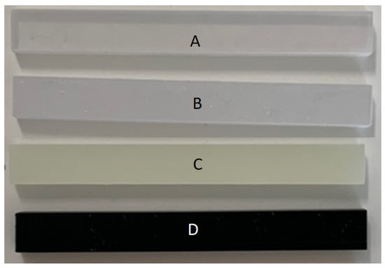
Figure 1. Specimens.

Table 1. Chemical components of polymer materials tested.

Materials	Chemical Name	%
	Isobornyl acrylate	30–40
Polymer A	4-(1-Oxo-2-propenyl)-morpholine	10–20
	Diphenyl (2,4,6-trimethyl-benzoyl)phosphine oxide	0.5–1.5
	2-Propenoic acid, 3-[2,2-dimethyl-1-oxo-3-[(1-oxo-2-propen-1-yl) oxy]propoxy]-2,2-dimethylpropyl ester	15–25
	Tricyclodecane dimethanol diacrylate	10–20
Polymer B	Diphenyl (2,4,6-trimethyl-benzoyl)phosphine oxide	0.5–1.5
	Isobornyl methacrylate	15–25
	2-Propenoic acid, 2-[[(butylamino)carbonyl]oxy]ethyl ester	25–35
	2-Propenoic acid, 1,1${}^{\prime }$-[(octahydro-4,7methano-1Hindene-5,?-diyl)bis(methylene)] ester	50–90
Polymer C	2-Propenoic acid, 2-methyl-, (1R,2R,4R)-1,7,7 trimethylbicyclo [2.2.1]hept2-yl ester, rel-	5–10
	diphenyl (2,4,6- trimethylbenzoyl) phosphine oxide	1–5
	2-Propen-1-one, 1-(4-morpholinyl)	30–50
Polymer D	2-Propenoic acid, 2-methyl-, (1R,2R,4R)-1,7,7 trimethylbicyclo [2.2.1]hept2-yl ester, rel-	5–25
	3,3,5-Trimethylcyclohexyl acrylate	5–10
	Phosphine oxide, phenylbis(2,4,6- trimethylbenzoyl)	1–10

3.2. Single Frequency Test

The glass transition temperature ($T_g$) is the temperature at which polymers change from rigid glassy materials to soft materials. That is a direct measurement of molecular mobility because of a reduction in motion of large segments of molecular chains with decreasing temperature. Dynamic mechanical analysis is one analytical technique used to determine $T_g$. The glass transition occurs over a range of temperatures and is not a point or single temperature. In general, the intercept from the glassy plateau of the storage modulus and the line after the sudden drop of the storage modulus in the transition region, the peak of loss modulus, or the peak of loss tangent are considered as $T_g$s. Frequency and temperature are considered the key variables in the study of the dynamic mechanical properties of polymers.

Based on the single frequency test, the glass transition temperature was measured. In this study, dynamic measurements were carried out over a temperature range at constant frequency. A TA Instruments Q800 dynamical mechanical analyzer (DMA) was used to measure the glass transition temperature ($T_g$) of the specimens. A single cantilever was used at a frequency of 1 Hz, an amplitude of 25 microns/meter, and a ramp rate of 2 ${}^{°}$C/min. Initially, it was equilibrated isothermally at −120 ${}^{°}$C for 10 min. Then, the temperature was increased by 2 ${}^{°}$C/min. The $T_g$ measured was also used to determine the test window for the temperature–frequency sweep test.

3.3. Frequency Sweep Test

In this test, dynamic measurements were carried out over a frequency range under isothermal conditions and the storage modulus vs. frequency curve was obtained. The frequency range from 0.1 to 100 Hz and 10 MPa stress were used. This tests were conducted in the temperature range from 20 to 100 ${}^{°}$C, increasing by 5 ${}^{°}$C.

4. Results and Discussion

4.1. Glass Transition Temperature

The effects of temperature on the dynamic moduli and the loss tangent measured for four polymers are illustrated in Figure 2, Figure 3, Figure 4 and Figure 5. Figure 2 shows the storage modulus of Polymer A at various temperatures. According to the single frequency test, the glass transition temperature of Polymer A was measured as 64.79 ${}^{°}$C. The lower the temperature, the higher the storage modulus, and the wider the range of change around the glass transition temperature. Table 2 shows the glass transition temperature ($T_g$) measured at the peak of the tangent delta for the polymers. The glass transition temperatures of Polymer C and Polymer D were 159.91 and 109.11 ${}^{°}$C, respectively. However, the $T_g$s of Polymer A and Polymer B were around 65 ${}^{°}$C. Therefore, Polymer C and Polymer D could be suitable to use at a service temperature near 100 ${}^{°}$C or above. In addition, the onset point of the storage modulus obtained through this test was used to set the temperature region in the next frequency sweep test.

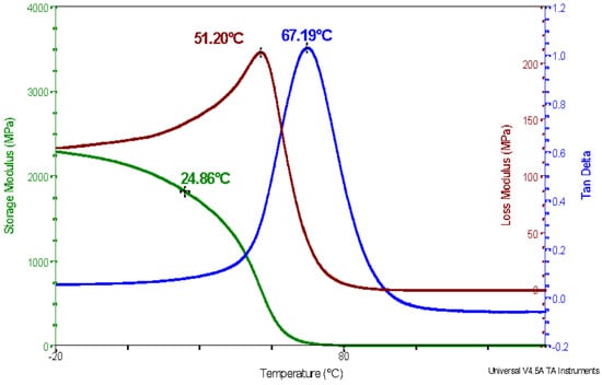
Figure 2. Thermal analysis curve of Polymer A obtained from single-frequency test.

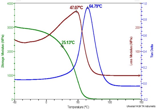
Figure 3. Thermal analysis curve of Polymer B obtained from single-frequency test.

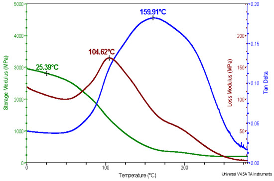
Figure 4. Thermal analysis curve of Polymer C obtained from single-frequency test.

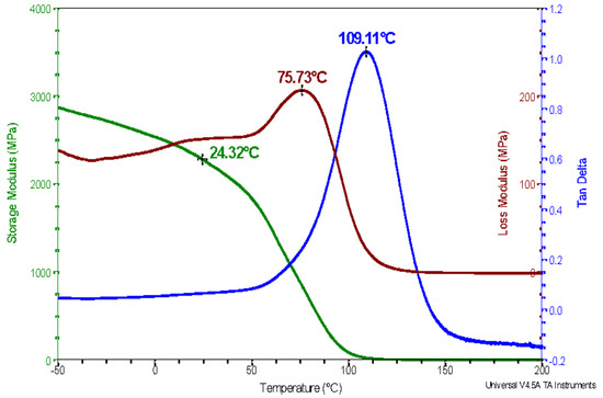
Figure 5. Thermal analysis curve of Polymer D obtained from single-frequency test.

Table 2. Glass transition temperature ($T_g$) for 3D-printed polymers.

3D Printing Technique	Material	${\mathit{T}}_{\mathit{g}}$ [${}^{°}$C]
MultiJet Printing (MJP)	Polymer A	67.19
	Polymer B	64.79
	Polymer C	159.91
Digital Lighting Process (DLP)	Polymer D	109.11

4.2. Complex Moduli in the Frequency Domain

Figure 6, Figure 7, Figure 8 and Figure 9 show the storage modulus curves of Polymers A, B, C, and D, respectively, which were measured under isothermal conditions over a frequency range from 0.1 to 100 Hz. It was observed that the storage moduli were increased with frequency increase, while they were decreased with temperature increase.

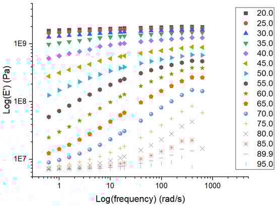
Figure 6. Storage modulus of Polymer A at various temperatures.

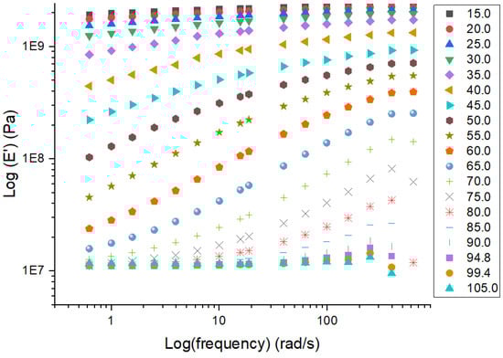
Figure 7. Storage modulus of Polymer B at various temperatures.

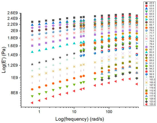
Figure 8. Storage modulus of Polymer C at various temperatures.

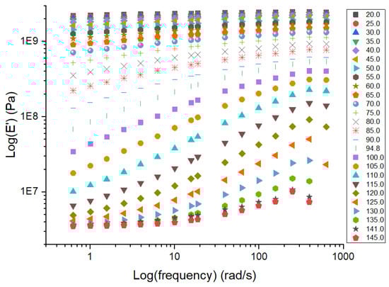
Figure 9. Storage modulus of Polymer D at various temperatures.

The storage moduli curves measured at different temperatures can be superposed into master curves using the frequency–temperature superposition principle. The superposition principle states that the storage modulus at one temperature can be related to another one at different temperatures by a change in the frequency scale only. The shift factors defined in Equation (3) for Polymers A, B, C, and D were calculated as a function of temperature.

Williams, Landel, and Ferry [14] observed that many polymers exhibit similar temperature-dependent behaviors and proposed an empirical shift function relationship:

$$log{a}_T=\frac{-C_1(T-T_r)}{C_2+(T-T_r)}$$

(8)

where $a_T$ is the shift function, $C_1$ and $C_2$ are universal parameters that vary from polymer to polymer, T is the temperature, and $T_r$ is the reference temperature of the master curve.

In this study, those shift factors were curve-fitted to Equation (8). Figure 10, Figure 11, Figure 12 and Figure 13 show the shift factors of Polymers A, B, C, and D, respectively, and the measured shift factors were compared with the curve-fitted ones. The WLF parameters, $C_1$s and $C_2$s, are given in Table 3. As shown in Figure 10, Figure 11, Figure 12 and Figure 13, those shift factors were well-represented by the WLF equation.

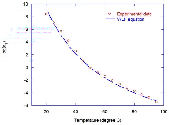
Figure 10. Shift factors of Polymer A.

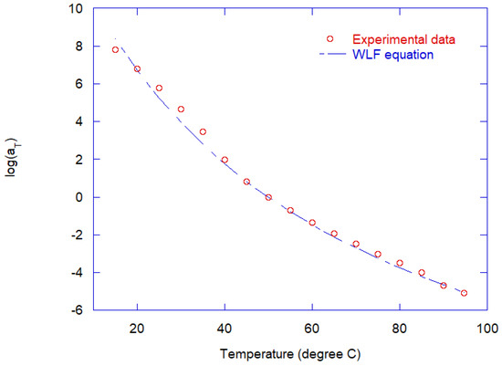
Figure 11. Shift factors of Polymer B.

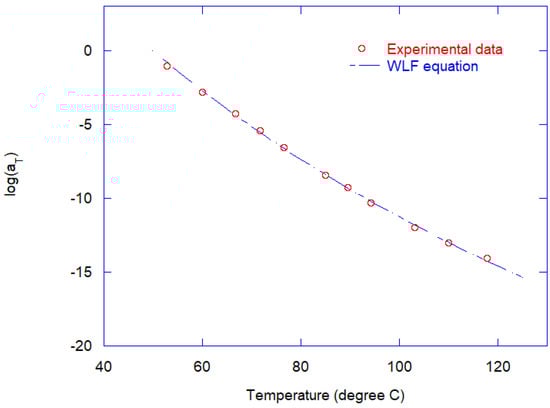
Figure 12. Shift factors of Polymer C.

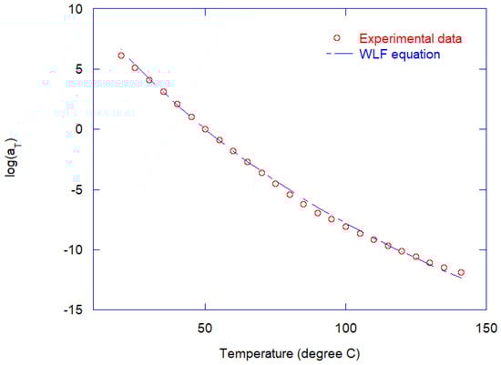
Figure 13. Shift factors of Polymer D.

Table 3. WLF factors at reference temperature 50 ${}^{°}$C.

Materials	${\mathit{C}}_1$	${\mathit{C}}_2$
Polymer A	13.56	75.21
Polymer B	15.67	99.75
Polymer C	57.45	205.3
Polymer D	42.83	224.9

The master curves of Polymers A, B, C, and D at reference temperature 50 ${}^{°}$C are illustrated in Figure 14, Figure 15, Figure 16 and Figure 17, respectively. These curves were obtained by shifting the curve with the shift factor defined in Equation (3).

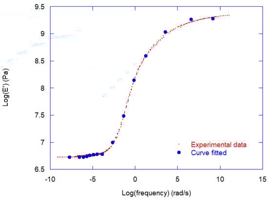
Figure 14. Master storage modulus of Polymer A.

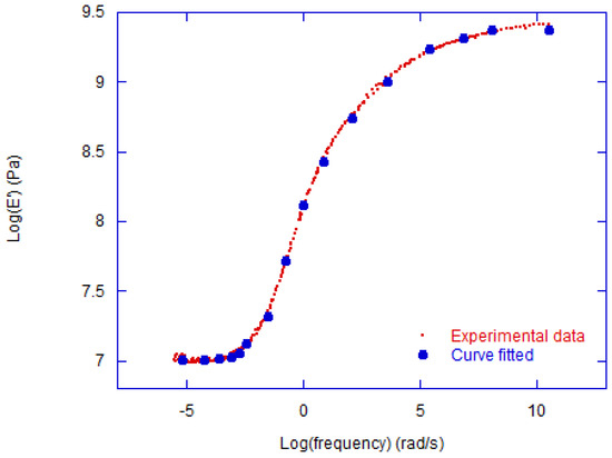
Figure 15. Master storage modulus of Polymer B.

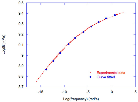
Figure 16. Master storage modulus of Polymer C.

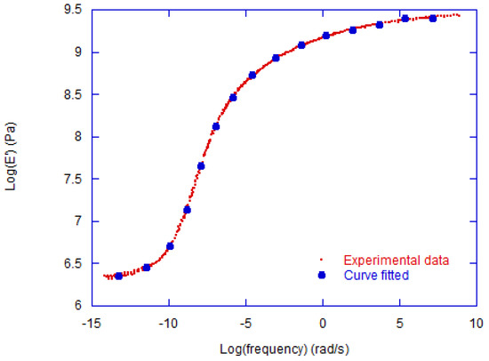
Figure 17. Master storage modulus of Polymer D.

4.3. Relaxation Moduli in the Time Doain

Equations (6) and (7) may be recognized as Fourier sin and cosine transforms, respectively. The relaxation modulus $E\left(t\right)$ can be obtained by taking the inverse Fourier transform of Equation (6) as:

$$\begin{array}{c}\hfill E(\mathbf{x},t)=\frac{2}{\pi }{\int }_0^{\infty }\frac{{\overline{\overline{E}}}_R(\mathbf{x},\omega )}{\omega }sin\left(\omega t\right)dt\omega \end{array}$$

(9)

The dynamic complex results shown in Figure 14, Figure 15, Figure 16 and Figure 17 can be readily converted into time-dependent functions. The stress relaxation modulus, $E\left(t\right)$, can be obtained by using the inverse fast Fourier transform (IFFT) of the complex results. However, in general, IFFT is very time-consuming and often the accuracy of the classical IFFT algorithm is questionable [15]. Ninomiya and Ferry [16] introduced some approximation methods to obtain the relaxation (or creep) function from the real and imaginary parts of the complex modulus.

In this study, the complex moduli curves that were measured in the frequency were then curve-fitted onto generalized Maxwell models by using the least squares method (see [13]). For generalized Maxwell models, the relaxation moduli for viscoelastic materials can be defined by the Prony or Dirichlet series as [13,17]:

$$E(\mathbf{x},t)=\sum _{i=1}^N{E}_i\left(\mathbf{x}\right)·exp(-t/{\lambda }_i)$$

(10)

where N is the number of series terms and $\lambda$s are relaxation times. For computational purposes, the relaxation modulus in Equation (9) can be expanded in terms of Prony series summations. Then, in the frequency domain, we have:

$${\overline{\overline{E}}}_R(\mathbf{x},\omega )=\sum _{i=1}^N\frac{{\omega }^2{\lambda }_i^2{E}_i\left(\mathbf{x}\right)}{1+{\omega }^2{\lambda }_i^2}$$

(11)

By using the least square method that minimizes the sum of deviation, $E_i$ and ${\lambda }_i$ were determined. The experimental results for Polymers A, B, C, and D and those curve-fitted are depicted in Figure 14, Figure 15, Figure 16 and Figure 17. Excellent agreement was obtained between the experimental results and those curve-fitted within less than $0.5\%$ error. $E_i$ and ${\lambda }_i$ for Polymers A, B, C, and D are tabulated in Table 4, Table 5, Table 6 and Table 7, respectively.

Table 4. $E_i$ and ${\lambda }_i$ for Polymer A.

No.	${\mathit{E}}_{\mathit{i}}$	${\mathit{\lambda }}_{\mathit{i}}$
1	6.83 × 10${}^8$	7.38 × 10${}^{-7}$
2	6.49 × 10${}^8$	5.41 × 10${}^{-4}$
3	3.39 × 10${}^8$	5.22 × 10${}^{-2}$
4	1.79 × 10${}^8$	1.20 × 10${}^0$
5	4.58 × 10${}^7$	1.79 × 10${}^1$
6	3.34 × 10${}^{-1}$	1.76 × 10${}^2$
7	6.63 × 10${}^6$	5.19 × 10${}^2$
8	2.92 × 10${}^1$	9.67 × 10${}^4$
9	7.02 × 10${}^5$	3.31 × 10${}^5$
10	9.57 × 10${}^{-4}$	1.00 × 10${}^{12}$
11	9.42 × 10${}^4$	1.46504 × 10${}^{14}$
12	5.30 × 10${}^6$	∞

Table 5. $E_i$ and ${\lambda }_i$ for Polymer B.

No.	${\mathit{E}}_{\mathit{i}}$	${\mathit{\lambda }}_{\mathit{i}}$
1	6.31 × 10${}^8$ × 10${}^8$	1.38 × 10${}^{-7}$
2	7.11 × 10${}^8$	3.65 × 10${}^{-5}$
3	4.88 × 10${}^8$	2.14 × 10${}^{-3}$
4	3.09 × 10${}^8$	6.51 × 10${}^{-2}$
5	1.53 × 10${}^8$	9.61 × 10${}^{-1}$
6	3.78 × 10${}^7$	1.18 × 10${}^1$
7	6.75 × 10${}^6$	2.47 × 10${}^2$
8	9.67 × 10${}^2$	2.97 × 10${}^7$
9	1.02 × 10${}^7$	∞

Table 6. $E_i$ and ${\lambda }_i$ for Polymer C.

No.	${\mathit{E}}_{\mathit{i}}$	${\mathit{\lambda }}_{\mathit{i}}$
1	2.19 × 10${}^8$	3.47 × 10${}^{-1}$
2	1.91 × 10${}^8$	5.31 × 10${}^1$
3	1.99 × 10${}^8$	3.65 × 10${}^3$
4	2.17 × 10${}^8$	1.93 × 10${}^5$
5	1.91 × 10${}^8$	8.15 × 10${}^6$
6	1.96 × 10${}^8$	2.84 × 10${}^8$
7	2.18 × 10${}^8$	1.10 × 10${}^{10}$
8	1.76 × 10${}^8$	5.20 × 10${}^{11}$
9	1.50 × 10${}^8$	1.66 × 10${}^{13}$
10	1.63 × 10${}^8$	7.19 × 10${}^{14}$
11	5.63 × 10${}^8$	∞

Table 7. $E_i$ and ${\lambda }_i$ for Polymer D.

No.	${\mathit{E}}_{\mathit{i}}$	${\mathit{\lambda }}_{\mathit{i}}$
1	4.16 × 10${}^8$	1.15 × 10${}^{-5}$
2	4.47 × 10${}^8$	7.50 × 10${}^{-3}$
3	4.20 × 10${}^8$	1.13 × 10${}^0$
4	3.78 × 10${}^8$	8.33 × 10${}^1$
5	3.24 × 10${}^8$	3.91 × 10${}^3$
6	2.36 × 10${}^8$	1.12 × 10${}^5$
7	1.70 × 10${}^8$	1.73 × 10${}^6$
8	9.83 × 10${}^7$	1.77 × 10${}^7$
9	3.42 × 10${}^7$	1.57 × 10${}^8$
10	8.25 × 10${}^6$	1.51 × 10${}^9$
11	2.17 × 10${}^6$	1.97 × 10${}^{10}$
12	6.52 × 10${}^5$	1.01 × 10${}^{12}$
13	2.27 × 10${}^6$	∞

The master curves of relaxation moduli $E\left(t\right)$s for Polymers A, B, C, and D at reference temperature 50 ${}^{°}$C are shown in Figure 18. The time domain curves show mirror images of the frequency domain curves. As shown in Figure 18, the relaxation modulus curves show glassy, transition, and rubbery states. At low temperatures or high frequencies, polymers are hard and brittle and behave like elastic materials. In the glassy region, the modulus is not degraded with time and corresponds to the elastic one. As time or temperature increases, material behavior moves to the transition region where the material properties are very rapidly degraded with time and temperature. As time or temperature are further increased, the modulus reaches another plateau region that is called the rubbery region and where the modulus reaches the so-called relaxed value.

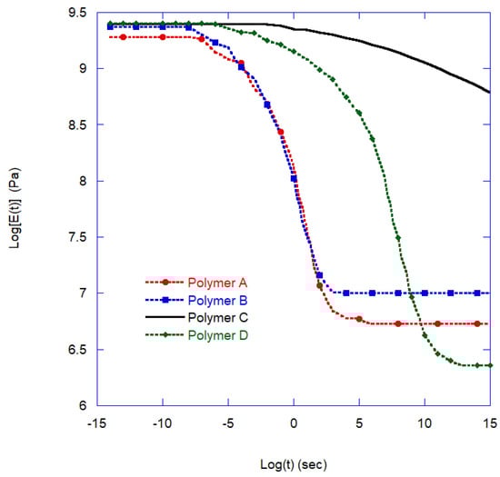
Figure 18. Master relaxation curves.

As shown in Figure 18, after about a year, the moduli of Polymers A, B, and D decreased by 90%, 96%, and 96%, respectively, while the modulus of Polymer C was reduced by 34% only. The equilibrium modulus, $E(\infty )$, of Polymer C was 5.63 × 10${}^8$ Pa, which was much larger than ones of Polymers A, B, and D. Polymer C was highly crosslinked. Among the four materials, Polymer C showed low modulus reduction after about a year. The experimental results show that the crosslinks of Polymer C were higher than ones of Polymers A, B, and D.

5. Conclusions

In this study, a single-frequency test and a frequency sweep test were performed on four different polymers used for 3D printing methods such as multi-jet printing and digital lighting process. The glass transition temperature was determined by using a single-frequency test. Dynamic measurements were carried out over a frequency range under isothermal conditions and storage modulus vs. frequency curves were obtained. Then, the master curves of relaxation moduli at a reference temperature were obtained by curve-fitting the complex moduli curves onto generalized Maxwell models using the least squares method. The effects of temperature, frequency, and time on dynamic moduli and the relaxation behaviors of polymers used for 3D printing were evaluated. The glass transition temperatures of Polymers C and D were 159.91 and 109.11 ${}^{°}$C, respectively, while those of Polymers A and B were around 65 ${}^{°}$C. Therefore, Polymers C and D could be suitable to use at a service temperature above 100 ${}^{°}$C. After about a year, the moduli of Polymers A, B, and D decreased by 90%, 96%, and 96%, respectively, while the modulus of Polymer C was reduced by 34% only. The equilibrium modulus, $E(\infty )$, of Polymer C was 5.63 × 10${}^8$ Pa, which was much larger than ones of Polymers A, B, and D. Polymer C was highly crosslinked and showed low modulus reduction after about a year. The master relaxation curves obtained through this process can be utilized to predict the long-term performance of polymer molds made by 3D printing at a given environmental condition.

References

- Oroszlany, A.; Nagy, P.; Kovacs, J. Injection molding of degradable interference screws into polymeric mold. Mate. Sci. Forum 2010, 659, 73–77. [Google Scholar] [CrossRef]
- Volpato, N.; Solis, D.; Costa, C. An analysis of digital abs as a rapid tooling material for polymer injection moulding. Int. J. Mater. Prod. Technol. 2016, 52, 3–16. [Google Scholar] [CrossRef]
- Nelson, J.; LaValle, J.; Kautzman, B.; Dworshak, J.; Johnson, E.; Ulven, C. Injection molding with an additive manufacturing tool: Study shows that 3D-printed tools can create parts comparable to those made with p20 tools, at a much lower cost and lead time. Plastics Eng. 2017, 73, 60–66. [Google Scholar] [CrossRef]
- Mendible, G.A.; Rulander, J.A.; Johnston, S.P. Comparative study of rapid and conventional tooling for plastics injection molding. Rapid Prototyp. J. 2017, 23, 344–352. [Google Scholar] [CrossRef]
- Ngo, T.; Kashani, A.; Imbalzano, G.; Nguyen, K.; Hui, D. Additive manufacturing (3D printing): A review of materials, methods, applications and challenges. Compos. Part B 2018, 143, 172–196. [Google Scholar] [CrossRef]
- Kampker, A.; Triebs, J.; Alves, B.; Kawollek, S.; Ayvaz, P. Potential analysis of additive manufacturing technologies for fabrication of polymer tools for injection moulding; A comparative study. In Proceedings of the 2018 IEEE International Conference on Advanced Manufacturing (ICAM), Yunlin, Taiwan, 16–18 November 2018; pp. 49–52. [Google Scholar]
- Kuo, C.C.; Tasi, Q.Z.; Hunag, S.H. Development of an Epoxy-Based Rapid Tool with Low Vulcanization Energy Consumption Channels for Liquid Silicone Rubber Injection Molding. Polymers 2022, 14, 4534. [Google Scholar] [CrossRef] [PubMed]
- Yi, S. Thermoviscoelastic Analysis of Delamination Onset and Free Edge Response in Epoxy Matrix Composite Laminates. AIAA J. 1993, 31, 2320–2328. [Google Scholar] [CrossRef]
- Hussin, R.B.; Sharif, S.B.; Abd Rahim, S.Z.B.; Suhaimi, M.A.B.; Bin Mohd Khushairi, M.T.; Abdellah EL-Hadj, A.; Shuaib, N.A.B. The potential of metal epoxy composite (MEC) as hybrid mold inserts in rapid tooling application: A review. Rapid Prototyp. J. 2021, 27, 1069–1100. [Google Scholar] [CrossRef]
- Chatterjee, D.; Jafferson, J.M. A review on polymeric materials in additive manufacturing. Mater. Today Proc. 2021, 46, 1349–1365. [Google Scholar]
- Abdulhameed, O.; Al-Ahmari, A.; Wadea Ameen, W.; Mian, S. Additive manufacturing: Challenges, trends, and applications. Adv. Mech. Eng. 2019, 11, 1–27. [Google Scholar] [CrossRef]
- Hilton, H.H.; Russell, H.G. An Extension of Alfrey’s Analogy to Thermal Stress Problems in Temperature-Dependent Linear Viscoelastic Media. J. Mech. Phys. Solids 1961, 9, 152–164. [Google Scholar] [CrossRef]
- Hilton, H.H.; Yi, S. Analytic Formulation of Optimum Material Properties for Viscoelastic Damping. Smart Mater. Struct. 1992, 1, 113–122. [Google Scholar] [CrossRef]
- Williams, M.; Landel, R.; Ferry, J. The Temperature Dependence of Relaxation Mechanisms in Amorphous Polymers and Other Glass-forming Liquids. J. Am. Chem. Soc. 1955, 77, 3701–3707. [Google Scholar] [CrossRef]
- Lovrić, D.; Vujević, S.; Sarajĉev, P. Accuracy of the Inverse Fast Fourier Transform algorithm in grounding grid transient analysis. In Proceedings of the 2010 Proceedings ICECom, 20th International Conference on Applied Electromagnetics and Communications, Dubrovnik, Croatia, 20–23 September 2010; pp. 1–4. [Google Scholar]
- Ninomiya, K.; Ferry, J.D. Some approximate equations useful in the phenomenological treatment of linear viscoelastic data. J. Colloid Sci. 1959, 14, 36–48. [Google Scholar] [CrossRef]
- Yi, S.; Hilton, H.H. Dynamic Finite Element Analysis of Viscoelastic Composite Plates. Int. J. Numer. Methods Eng. 1994, 37, 4081–4096. [Google Scholar] [CrossRef]
Disclaimer/Publisher’s Note: The statements, opinions and data contained in all publications are solely those of the individual author(s) and contributor(s) and not of MDPI and/or the editor(s). MDPI and/or the editor(s) disclaim responsibility for any injury to people or property resulting from any ideas, methods, instructions or products referred to in the content. |
© 2023 by the authors. Licensee MDPI, Basel, Switzerland. This article is an open access article distributed under the terms and conditions of the Creative Commons Attribution (CC BY) license (https://creativecommons.org/licenses/by/4.0/).