Article

Accurate Extraction of Cableways Based on the LS-PCA Combination Analysis Method

by
Wenxin Wang
1,2,*,†,‡,
Changming Zhao
1,2,†,‡ and
Haiyang Zhang
1,2,†
1
Key Laboratory of Photoelectronic Imaging Technology and System, Ministry of Education, Beijing 100081, China
2
Key Laboratory of Photonics Information Technology, Ministry of Industry and Information Technology, Beijing 100081, China
*
Author to whom correspondence should be addressed.
Current address: School of Optics and Photonics, Beijing Institute of Technology, Beijing 100081, China.
These authors contributed equally to this work.
Appl. Sci. 2023, 13(5), 2875; https://doi.org/10.3390/app13052875
Submission received: 31 January 2023 / Revised: 17 February 2023 / Accepted: 21 February 2023 / Published: 23 February 2023
(This article belongs to the Section Optics and Lasers)

Abstract

:
In order to maintain a ski resort efficiently, regular inspections of the cableways are essential. However, there are some difficulties in discovering and observing the cable car cableways in the ski resort. This paper proposes a high-precision segmentation and extraction method based on the 3D laser point cloud data collected by airborne lidar to address these problems. In this method, first, an elevation filtering algorithm is used to remove ground points and low-height vegetation, followed by preliminary segmentation of the cableway using the spatial distribution characteristics of the point cloud. The ropeway segmentation and extraction are then completed using the least squares-principal component combination analysis method for parameter fitting. Additionally, we selected three samples of data from the National Alpine Ski Center to be used as test objects. The real value is determined by the number of point clouds manually deducted by CloudCompare. The extraction accuracy is defined as the ratio of the number of point clouds extracted by the algorithm to the number of point clouds manually extracted. While the environmental complexities of the samples differ, the algorithm proposed in this paper is capable of segmenting and extracting cableways with great accuracy, achieving a comprehensive and effective extraction accuracy rate of 90.59%, which is sufficient to meet the project’s requirements.

1. Introduction

Globally, the ski industry has experienced rapid growth in recent years [1,2,3]. Whether it is the number of people participating in skiing or the number of new ski resorts, new records have been set [4,5,6,7]. Moreover, many ski resorts are equipped with multiple cableways of different types in order to improve user experiences. For the safety of customers, regular inspection and maintenance of cable cars are integral to the daily operation and maintenance of a ski resort. A significant part of the daily maintenance process involves the observation and inspection of cable car cables. In severe cases, faulty or damaged cables can result in cable cars malfunctioning and the cableway breaking, resulting in a serious safety accident. Figure 1 illustrates the distribution of cables.
Ropeway detection of cable cars can be accomplished in two ways [8,9,10]. Maintenance personnel can either observe with their naked eyes on the ground or use handheld devices to conduct manual inspections from a helicopter as the first measure. However, this detection method has several disadvantages, including the need for a large amount of manpower, material resources, and financial resources. As a second option, maintenance personnel may use drones equipped with smart sensors to carry out intelligent detection, in order to collect various types of data such as images and point clouds. This method is highly intelligent, convenient to operate, low cost, and easy to implement [11,12]. However, current mainstream image-based detection methods have many limitations, including the difficulty of segmenting cableways due to complex backgrounds and the inability to identify them due to blurry images or low pixel counts [13,14]. Therefore, based on the high-precision point cloud data collected by the UAV-borne 3D lidar system, many of the limitations of other detection methods can be overcome through its high positioning accuracy and strong anti-interference capability [15,16,17,18].
Many scholars have recently conducted research on the segmentation, detection, and information extraction of airborne lidar point clouds [19,20,21,22]. A support vector machine (SVM) classifier was used by Zhang et al. to identify cables, but there was a problem with misclassification when vegetation was planted below the cables [23]. The algorithm developed by Jiwa et al. began with meshing the point cloud, was then transformed using the Hough transform, and then point cloud features were used to extract cables, but the robustness of the algorithm was heavily reliant on the density of the point cloud [24]. A spatial grid and clustering method were used by Cheng et al. to extract cables; however, this method requires a large number of empirical values and cannot be fully automated [25]. The filtering method was used by Yu et al. in order to eliminate ground points, vegetation points, and building points; a Hough transform was then applied in order to separate a single cable [26]. This method will have classification errors regarding vegetation or other small objects under the cable. Based on the spatial dimension characteristics of the cable combined with the Hough transform method, Chen et al. were able to extract the cable after filtering out the ground points; however, this method requires calculating eigenvalues for each point, and there is incomplete segmentation at the rod body connection [27]. Furthermore, research on orthogonal polynomials will assist in the extraction of cable characteristics [28,29].
A method for high-precision segmentation and extraction of ropeways based on an adaptive algorithm is proposed in this paper in response to the difficult problem of ropeway observation and maintenance. This method consists of two stages: preprocessing cableway data and segmenting and extracting cableway data. At the preprocessing stage, the original ropeway data are filtered and the preliminary segmentation of the cableway is primarily performed through adaptive processing. During the cableway segmentation and extraction stage, the high-precision segmentation and extraction of the cableway are completed; the ropeway point clouds are separated from the non-ropeway point clouds and saved in separate files.
In summary, our main contributions are as follows:
  • We introduce spatial geometric distribution and an entropy function. The segmented upper part is further segmented based on the principle of spatial geometric distribution and the minimization of the entropy function.
  • We propose a comprehensive analysis. The final cable extraction is achieved by combining the least squares method and the principal component analysis method.
  • We carried out experimental verification. Three groups of samples were selected as the experimental objects, and the experimental results confirmed the efficacy of the proposed method as well as its reliability.

2. Methodology

2.1. Overview

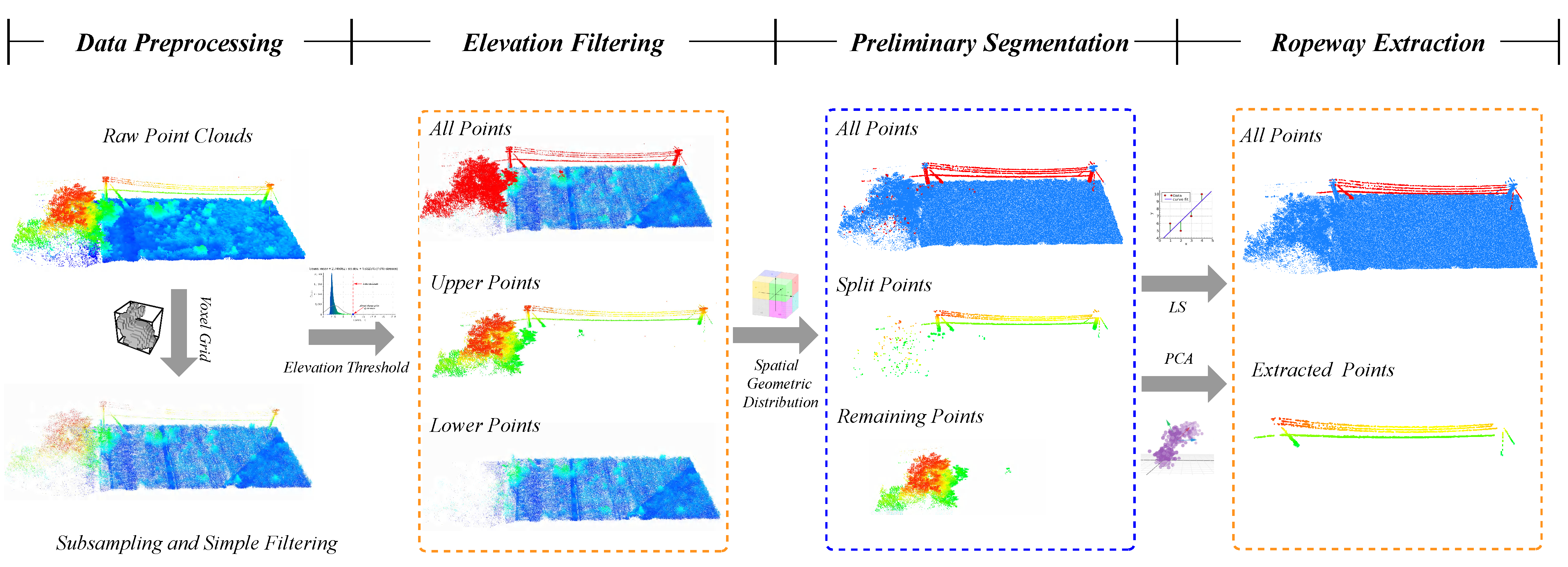
There are difficult problems associated with the observation and maintenance of cableways in ski resorts on a daily basis. Considering the above situation, we propose a high-precision segmentation and extraction method that provides convenience for the daily maintenance of the cableway. The raw point cloud is segmented based on an elevation threshold into upper and lower parts (Section 2.2.1).
Based on the spatial geometric distribution characteristics of the point clouds, the upper part of the point cloud is further segmented to complete the preliminary segmentation of the cables (Section 2.2.2). Finally, we use a combination of least squares and the principal component analysis to complete the final cable extraction (Section 2.3). The full pipeline is illustrated in Figure 2.

2.2. Preprocessing of Ropeway Data

The cable car cableway of the ski resort is a typical artificial construction, which has the following characteristics when viewed from the point cloud perspective:
  • In general, the ropeway extends linearly in a narrow and long shape, with a length much greater than a width;
  • There are no obvious objects around the cableway from a local perspective, and the individual cables are parallel to each other and maintain a certain distance from one another;
  • While cableway points have a discontinuous distribution in the vertical direction, they are closely connected in the horizontal direction.
Preprocessing operations on the original point cloud data are required in order to segment and extract the ropeways based on the above distribution characteristics. These operations include object removal, noise filtering, etc.
In the preprocessing section of this paper, the elevation filtering method is first applied in order to remove ground points and low object points. In addition to the ropeway point clouds, the filtered point clouds contain some tower points, high vegetation points, and noise points. In the next step, the cableway is preliminarily segmented based on the features of the point cloud in terms of spatial dimensions.

2.2.1. Filtering by Elevation

Elevation filtering is intended to remove the vast majority of ground objects from the complex original point cloud data, laying the groundwork for subsequent segmentation and extraction. In contrast to towers and ground object points, cableways are discontinuous in the vertical direction. In elevation filtering, low-ground objects and ground points are removed, linear structures (such as rivers and roads) are eliminated from the results of the cableway extraction, and redundant data are reduced. The following are the steps involved in the implementation:
  • The meshing of point clouds. This is divided into grids and all points within each grid are normalized to the horizontal plane of the grid’s lowest point, as shown in Figure 3a;
  • As shown in Figure 3b, the elevation threshold can be determined by drawing the “elevation-point-figure map” of the normalized point cloud;
  • Finally, the points within the target area and the points outside the target area are segmented based on their elevation threshold, as shown in Figure 3c.

2.2.2. Preliminary Segmentation of the Ropeway

After elevation filtering, the non-ground points include towers and some high-ground objects in addition to ropeway points. The tower consists of regular polygonal metal patches, while the point cloud in the local area has a regular surface pattern. The cableway can be described as a flexible cable chain. There is a linear distribution of point clouds in the local area, while vegetation points are irregular and scattered. Therefore, the cableway points can be extracted based on the geometric distribution of the point cloud space. By examining the three eigenvalues λ 1 , λ 2 and λ 3 λ 1 λ 2 λ 3 of the point set covariance matrix in the neighborhood of R, we can determine the geometric distribution characteristics of spatial points. When λ 1 λ 2 λ 3 , the target point shows a planar distribution feature, such as roads and towers, etc.; when λ 1 λ 2 λ 3 , the target point shows a linear distribution feature, such as cableway and road boundary, etc. When λ 1 λ 2 λ 3 , the target point can be divided into scattered and irregularly distributed point clouds, such as vegetation.
If a fixed neighborhood radius is used to estimate the local geometric features of points, it will result in large calculation errors, which will affect the segmentation results of the target points due to the uneven distribution of density in the point cloud. In order to determine the optimal neighborhood radius for solving the eigenvalue of each laser point, the probability a 1 D , a 2 D , a 3 D dimension characteristics of the three dimensions to which the target point belongs are defined as follows:
a 1 D , a 2 D , a 3 D = λ 1 λ 2 λ 1 , λ 2 λ 3 λ 1 , λ 3 λ 1
In Formula (1), a 1 D + a 2 D + a 3 D = 1 , Shannon entropy defines the amount of information contained in the neighborhood of this point as follows:
E f = a 1 D Ln a 1 D a 2 D Ln a 2 D a 3 D Ln a 3 D
As described in Formula (2), E f represents the amount of entropy contained in the neighborhood of the point, and the smaller this value, the less information the neighborhood contains, which means the more singular the dimensional feature of the point. The radius R with the minimum value of the function E f is the best neighborhood radius for this point when the radius interval R min , R max and radius increment R are set. The eigenvalue of each point is calculated using the adaptive neighborhood radius, and the preliminary extraction of the cableway point cloud is based on the relationship between the eigenvalues. The neighborhood radius interval should be selected based on the spatial range of the points showing the three characteristics. Radius increments should be based on the volume of point cloud data and the performance of the computer. The smaller the increment, the more time-consuming the process will be. In most cases, the radius increment for the filtered cableway point cloud extraction is 0.5, and the neighborhood radius interval is [ 1.4 , 2.8 ] .

2.3. Extraction of Ropeways

Further segmentation and extraction are performed on the cableway point cloud that has been initially obtained. By minimizing the sum of squared errors, the least squares method determines the best function-matching relationship between variables [30,31,32,33]. The results are affected by some “unfavorable” data since the method uses all data for calculations during data fitting. The principal component analysis (PCA) method was proposed by Hoppe in order to evaluate each sampling point’s “neighborhood” as well as to calculate normal vectors and plane fittings [34,35,36,37,38,39]. A PCA can be understood as geometric optimization of least squares, or as an equivalent of maximum likelihood estimation, and it is more accurate and efficient than least squares methods. This method is, therefore, widely used in the fitting of planes. A combination of the two algorithms is presented in this paper in order to mitigate the influence of “unfavorable” factors on point cloud data and increase the accuracy of feature extraction.

2.3.1. Least Square Method

Based on the assumption that the three-dimensional plane point data are P i x i , y i , z i ; i = 1 , , n , the fitting plane is defined as follows:
a x + b y + c z + d = 0
As shown in Formula (3), a , b , and c are plane parameters, d is the distance between the 3D scanning data point and the fitting plane, which is expressed as z = f ( x , y ) ; variance cumulative minimization in the z direction is as follows:
min i = 1 n r i 2 = min i = 1 n d vi 2 = min i = 1 n z i z ^ i 2
A residual r i d vi is a measure of the vertical distance between the fitted point z ^ i and the point z i . By using Formula (5), we determine the minimum of ij = a x ij + b y ij + c z ij + d 2 under the constraints of a 2 + b 2 + c 2 = 1 , which is the eigenvector M that corresponds to the minimum eigenvalue of matrix C.
C 3 × 3 = 1 n i = 1 n p i p ^ p i p ^ T
M = 1 n ij x ij , y ij , z ij , 1 T x ij , y ij , z ij , 1

2.3.2. Analyses Based on Principal Components

According to Formula (7), the covariance matrix of n points in a 3D point cloud data set P i x i , y i , z i ; i = 1 , , n can be calculated as follows:
C 3 × 3 = 1 n i = 1 n p i p ^ p i p ^ T
The plane equation would be as follows:
x cos α + y cos β + z cos γ + p = 0
a x + b y + c z = d , a 2 + b 2 + c 2 = 1
In this case, cos α , cos β , cos γ represent the cosines of the normal vector direction at point ( x , y , z ) on the plane, while | p | represents the distance from the origin to the plane. This is where Formula (8) is transformed into Formula (9), and the calculation of the plane equation is converted into the calculation of the four parameters a , b , c , and d. Data points x i , y i , z i are distanced from the plane as follows:
d i = a x i + b y i + c z i d
As a result, the problem of fitting the best plane to find the normal vector min d i 2 becomes the problem of finding the extremum:
f = i = 0 n d i 2 λ a 2 + b 2 + c 2 1
Formula (12) is obtained by calculating the partial derivative of f for the four unknown parameters a , b , c , d , and bringing the parameter d into Formula (11).
d i = a x i x ¯ + b y i y ¯ + c z i z ¯
Δ x i Δ x i Δ x i Δ y i Δ x i Δ z i Δ x i Δ y i Δ y i Δ y i Δ y i Δ z i Δ x i Δ z i Δ y i Δ z i Δ z i Δ z i a b c = λ a b c
As a result of the above formula, the parameter ( a , b , c ) T of the solution position can be viewed as an eigenvector, which corresponds to the eigenvalue λ , while the coefficient matrix represents the equivalent formula for the covariance matrix. Using Formula (9) and the characteristic equation A x = λ x , Formula (14) can be derived.
λ = i = 1 n a Δ x i + b Δ y i + c Δ z i 2 = i = 1 n d 2
The best plane fitting requires min d i 2 , which is the eigenvector A corresponding to the smallest eigenvalue of the coefficient matrix ( a , b , c ) T and also the solution vector corresponding to the smallest eigendecomposition of the covariance matrix (7).

2.3.3. Comprehensive Analysis

(1)
By utilizing the least squares method to fit the plane, we can obtain the plane formula a x + b y + c z + d = 0 and the distance d between each point of the point cloud and the fitting plane.
(2)
The error σ of the distance d obtained from (1) can be calculated for fitting the plane point cloud. If each point d i is far from 2 σ , delete it, otherwise keep it.
(3)
By performing a principal component analysis on the noise-removed point cloud data, the parameters of the fitting plane are obtained, and the eigenvalues are sorted by the basis size.
(4)
The ropeway point cloud is segmented and extracted according to the linear features of the points, and the extracted ropeway points are saved as ropeway points and the non-ropeway points as out-ropeway points.

3. Experiment and Results

3.1. Preparation of Experiments

To conduct this algorithm verification experiment, we selected Visual Studio 2019 as the development environment and PCL 1.11.1 as the dependent library, as shown in Table 1. This experimental platform has the following hardware configurations: an Intel i5 processor, 32GB of memory, and a Windows 11 operating system. We selected three samples from the point cloud of the National Alpine Skiing Center of the Beijing Winter Olympics to verify the cableway segmentation and extraction algorithm proposed in this study. The basic conditions of the three sample point clouds are shown in Table 2.
Three sets of ropeway sample data are segmented and extracted using the proposed method during the experiment. The original sample point cloud, the preprocessed point cloud, and the final extracted cableway point cloud are presented from both front and side angles for convenience of presentation. As well, the number of cableway point clouds extracted in this paper is counted, and the cableway point clouds are manually extracted with CloudCompare, then the two results are compared to determine the accuracy rate.

3.2. Experimental Results and Analysis

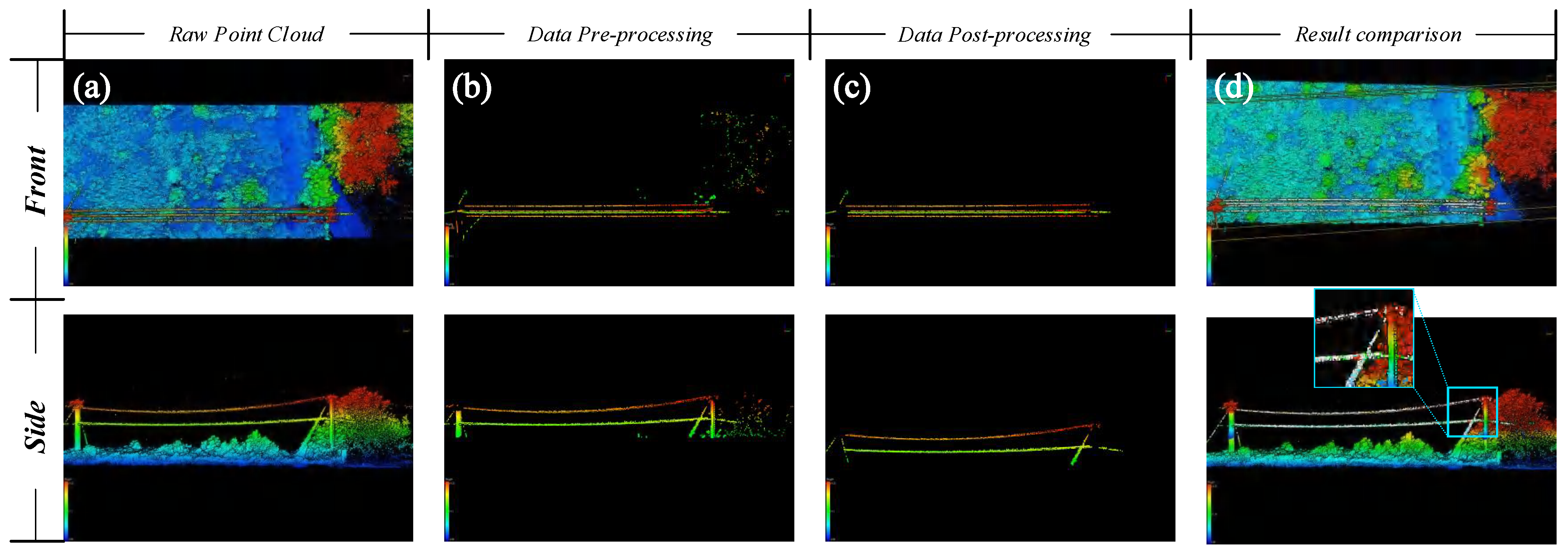
The three point cloud samples taken from the National Alpine Skiing Center of the Beijing Winter Olympics were extracted sequentially using the method proposed in this paper. Following the processing of the first set of sample data, the results are shown in Figure 4a–d.
Additionally, a gradient color is assigned to each sample point cloud based on its elevation. In Figure 4a, the front and side views of the first group of samples are shown before cableway segmentation and extraction. There is no doubt that the vegetation in the first group of samples is dense and some trees are tall, which presents great challenges in the extraction process. An illustration of the first set of samples after preliminary extraction is shown in Figure 4b. As shown in the figure, the point cloud obtained after preprocessing does not only include cables but also towers and vegetation point clouds that need to be further segmented and extracted. Based on the first set of samples, Figure 4c shows the front and side of the cableway segmented and extracted. From the figure, it is clear that whether viewed from the front or the side, the cableway point cloud has been well segmented and extracted. By fusing the two point clouds with different colors, the extracted ropeway and non-ropeway parts can be visually distinguished. In Figure 4d, the merged ropeway (white point) and non-ropeway (colored point) point clouds are represented as front and side views. As can be seen from the results of the first group of sample tests, the method proposed in this paper is effective in separating ropeway and non-ropeway components.
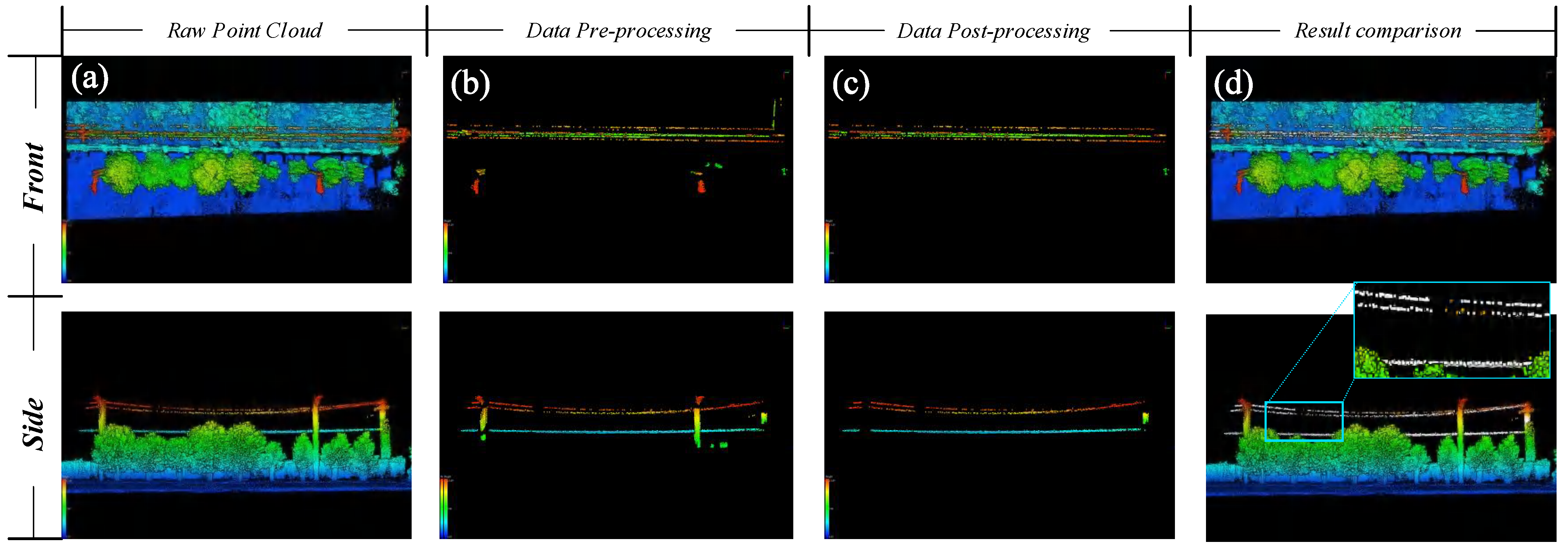
The second set of samples is then tested separately. When the proposed cableway point cloud segmentation and extraction algorithm is applied to the second group of samples, the following processing results are obtained as shown in Figure 5a–d.
As shown in Figure 5a, the second set of sample data is shown from both the front and side. The cableway will be difficult to extract due to some sporadic vegetation and trees in the picture. In Figure 5b, the front and side views of the second set of sample data after preprocessing are shown. The preprocessed data results are clearly superior, except for the cableway point cloud, which has only a few towers and vegetation point clouds. From the final segmentation and extraction of the second set of sample data, Figure 5c illustrates the front and side views of the cableway point cloud. The processing effect of this group of samples appears to be excellent. In Figure 5d, the ropeway point cloud (white) is compared with the non-ropeway point cloud (color). As can be seen intuitively, the method proposed in this paper still maintains good results in terms of segmenting and extracting cableway point clouds for the second set of test samples.
During the third set of test samples, we increased the complexity of the scene and the difficulty of processing the data. As part of the third set of data, tall light poles and trees with heights near the tower are also included, increasing the difficulty of segmenting and extracting cableways. The results of the data processing for the third group of samples are shown in Figure 6a–d.
Here are the front and side views of the third group of sample point clouds before data processing is performed, as shown in Figure 6a. This set of data contains a number of elements, including light poles and trees. Following data preprocessing, Figure 6b illustrates the front and side views of the data. There are still some light poles, towers, and vegetation point clouds that require further processing in the processed data. The Figure 6c shows the front and side views of the cableway point cloud obtained after segmentation and extraction. By this point, the ropeway segmentation and extraction of the third group of test samples have been completed. A comparison between the ropeway point cloud (white) and the non-ropeway point cloud (color) can be seen in Figure 6d. Performing ropeway segmentation and extraction on the third group of test samples demonstrates that the method proposed in this paper still performs at a high level.
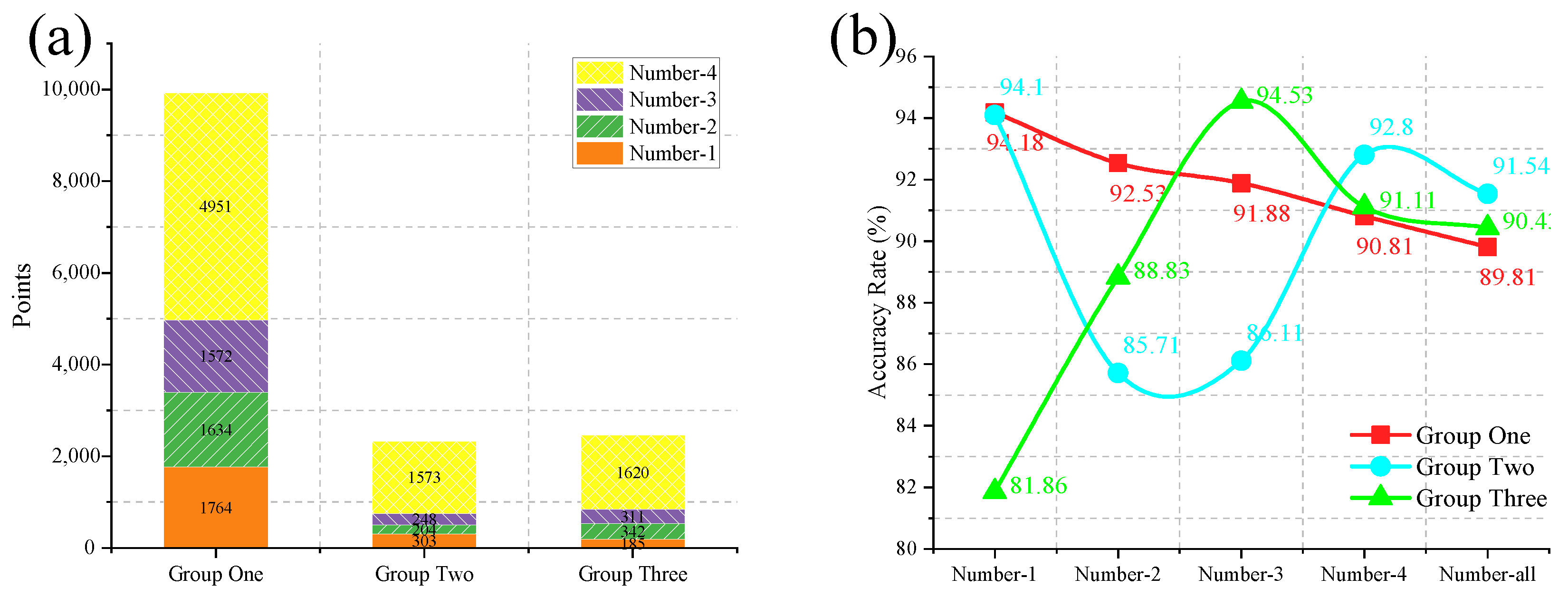
Next, the data will be compared with the cableway point cloud (considered to be the real value) extracted manually in order to quantitatively examine the extraction effect of the proposed method on the cableway point cloud in the three groups of test samples. As shown in Table 3 and Figure 7, the results of the data comparison are presented.
Three groups of sample point cloud data sets are processed using the ropeway segmentation and extraction method presented in this paper; the results of each group are compared with the real values in turn so that the accuracy of data extraction can be evaluated. Additionally, the extraction accuracy of the four cables in the three groups of test samples was compared as part of the comparison process. Table 3 and Figure 7 show that the extraction accuracy rate for each cable in the first group of test samples exceeds 90%, while the overall extraction rate reaches 89.81%; In the second group of samples, each cable’s accuracy rate was maintained above 85%, and the overall accuracy rate was 91.54%; Other than the first cable extraction accuracy rate of 81.86%, all other lines in the third group of samples have accuracy rates above 88%, and the overall accuracy rate is 90.43%. Accordingly, the effective extraction rate of this algorithm can reach 90.59%, maintaining a high level of extraction accuracy.
In order to further verify the effectiveness of the method proposed in this paper, we conducted cable extraction tests on five groups of samples sequentially using RF, GBDT, SVM, VBF-Net, and the proposed method. The extraction accuracy and extraction time of the test results are presented in Table 4 and Table 5, respectively (bold indicates the optimal result, underline indicates the suboptimal result, the arrow pointing up indicates that the larger the value is, the better, and the arrow pointing down indicates the smaller the value is, the better).
To facilitate the comparison of the extraction effects of different methods, a data analysis chart is generated, as shown in Figure 8. We found that our proposed method provides better results in terms of cable extraction accuracy and extraction time consumption.
The data processing of the above three groups of test samples was carried out using the self-adaptive high-precision segmentation and extraction algorithm presented in this paper. However, despite the differences in scene complexities among the groups of samples, the proposed method has a good segmentation effect, a high level of statistical accuracy, and is capable of accurately extracting the ropeway. Compared to other methods, the method presented in this paper has the advantage of being able to adjust the segmentation parameters adaptively as well as extract cableways fast and accurately. However, it should be noted that when selecting the elevation threshold, it must be classified according to the intended use. Otherwise, over-segmentation or under-segmentation may occur.

4. Conclusions

In order to locate and observe the cableway in the ski resort, this paper proposes an adaptive algorithm based on 3D point cloud data collected by airborne lidar to segment and extract the cableway with high precision. In this method, the process consists of two steps: preprocessing the ropeway data and segmenting and extracting the ropeway data. The cableway data preprocessing stage primarily focuses on denoising and pre-segmenting point cloud data based on spatial geometric distribution; the cableway data segmentation–extraction stage primarily focuses on completing the final snow track extraction based on the LS-PCA combination analysis method.
During the experimental verification stage, the three samples selected were all taken from the Beijing Winter Olympics National Alpine Skiing Center. Despite the differences in complexity between the three groups of samples, the algorithm described in this paper is capable of accurately segmenting and extracting the ropeway point cloud from the complex point cloud. Moreover, it has been determined that this algorithm can achieve an effective extraction rate of 90.59% based on the comprehensive test results. Consequently, compared to other methods, the expected result was achieved and lays the foundation for future inspections and maintenance of the cable car ropeways. In the future, we will increase our research on the semantic annotation and reconstruction of cables.

Author Contributions

Conceptualization, W.W. and H.Z.; methodology, W.W. and C.Z.; software, W.W.; validation, W.W., C.Z. and H.Z.; formal analysis, W.W.; investigation, W.W.; resources, C.Z.; data curation, W.W.; writing—original draft preparation, W.W.; writing—review and editing, C.Z.; visualization, W.W.; supervision, C.Z. and H.Z.; project administration, C.Z.; funding acquisition, C.Z. All authors have read and agreed to the published version of the manuscript.

Funding

This research was funded by the National Key R&D Program of China, a special project of the “Science and Technology Winter Olympics” (2018YFF0300802), and the National Natural Science Foundation of China (NSFC) (61378020, 61775018).

Institutional Review Board Statement

Not applicable.

Informed Consent Statement

Not applicable.

Data Availability Statement

Not applicable.

Acknowledgments

We thank the anonymous reviewers and members of the editorial team for their comments and contributions.

Conflicts of Interest

The authors declare no conflict of interest.

Abbreviations

The following abbreviations are used in this manuscript:
2D and 3Dtwo-dimensional and three-dimensional
UAVunmanned aerial vehicle
LiDARlight detection and ranging
PCLPoint Cloud Library
SVMsupport vector machine
PCAprincipal component analysis
LSleast square

References

  1. Gilaberte-Búrdalo, M.; López-Martín, F.; Pino-Otín, M.; López-Moreno, J.I. Impacts of climate change on ski industry. Environ. Sci. Policy 2014, 44, 51–61. [Google Scholar] [CrossRef] [Green Version]
  2. Scott, D.; McBoyle, G. Climate change adaptation in the ski industry. Mitig. Adapt. Strateg. Glob. Chang. 2007, 12, 1411–1431. [Google Scholar] [CrossRef]
  3. Duglio, S.; Beltramo, R. Environmental management and sustainable labels in the ski industry: A critical review. Sustainability 2016, 8, 851. [Google Scholar] [CrossRef] [Green Version]
  4. Wolfsegger, C.; Gössling, S.; Scott, D. Climate change risk appraisal in the Austrian ski industry. Tour. Rev. Int. 2008, 12, 13–23. [Google Scholar] [CrossRef]
  5. Hopkins, D. The sustainability of climate change adaptation strategies in New Zealand’s ski industry: A range of stakeholder perceptions. J. Sustain. Tour. 2014, 22, 107–126. [Google Scholar] [CrossRef]
  6. Rutty, M.; Scott, D.; Johnson, P.; Pons, M.; Steiger, R.; Vilella, M. Using ski industry response to climatic variability to assess climate change risk: An analogue study in Eastern Canada. Tour. Manag. 2017, 58, 196–204. [Google Scholar] [CrossRef]
  7. Hendrikx, J.; Zammit, C.; Hreinsson, E.; Becken, S. A comparative assessment of the potential impact of climate change on the ski industry in New Zealand and Australia. Clim. Chang. 2013, 119, 965–978. [Google Scholar] [CrossRef]
  8. Wen, T.; Hong, T.; Su, J.; Zhu, Y.; Kong, F.; Chileshe, J. Tension detection device for circular chain cargo transportation ropeway in mountain orchard. Nongye Jixie Xuebao = Trans. Chin. Soc. Agric. Mach. 2011, 42, 80–84. [Google Scholar]
  9. Ogura, K.; Nihonyanagi, K.; Katsuma, R. Rope Deployment Method for Ropeway-Type Vermin Detection Systems. In Proceedings of the 2018 IEEE 32nd International Conference on Advanced Information Networking and Applications (AINA), Krakow, Poland, 16–18 May 2018; pp. 350–357. [Google Scholar]
  10. Sukhorukov, V.V. Steel Rope Diagnostics by Magnetic NDT: From Defect Detection to Automated Condition Monitoring. Mater. Eval. 2021, 79, 438–445. [Google Scholar]
  11. Fathy, M.; Siyal, M.Y. An image detection technique based on morphological edge detection and background differencing for real-time traffic analysis. Pattern Recognit. Lett. 1995, 16, 1321–1330. [Google Scholar] [CrossRef]
  12. Liang, S.; Li, Y.; Srikant, R. Enhancing the reliability of out-of-distribution image detection in neural networks. arXiv 2017, arXiv:1706.02690. [Google Scholar]
  13. Chum, O.; Philbin, J.; Zisserman, A. Near duplicate image detection: Min-hash and TF-IDF weighting. BMVC 2008, 810, 812–815. [Google Scholar]
  14. Dosovitskiy, A.; Beyer, L.; Kolesnikov, A.; Weissenborn, D.; Zhai, X.; Unterthiner, T.; Dehghani, M.; Minderer, M.; Heigold, G.; Gelly, S.; et al. An image is worth 16x16 words: Transformers for image recognition at scale. arXiv 2020, arXiv:2010.11929. [Google Scholar]
  15. Zhou, Y.; Tuzel, O. Voxelnet: End-to-end learning for point cloud based 3d object detection. In Proceedings of the IEEE Conference on Computer Vision and Pattern Recognition, Salt Lake City, UT, USA, 18–23 June 2018; pp. 4490–4499. [Google Scholar]
  16. Schnabel, R.; Wahl, R.; Klein, R. Efficient RANSAC for point-cloud shape detection. Comput. Graph. Forum 2007, 26, 214–226. [Google Scholar] [CrossRef]
  17. Shi, S.; Wang, X.; Li, H. Pointrcnn: 3d object proposal generation and detection from point cloud. In Proceedings of the IEEE/CVF Conference on Computer Vision and Pattern Recognition, Long Beach, CA, USA, 15–20 June 2019; pp. 770–779. [Google Scholar]
  18. He, C.; Zeng, H.; Huang, J.; Hua, X.S.; Zhang, L. Structure aware single-stage 3d object detection from point cloud. In Proceedings of the IEEE/CVF Conference on Computer Vision and Pattern Recognition, Seattle, WA, USA, 13–19 June 2020; pp. 11873–11882. [Google Scholar]
  19. Fernandes, D.; Silva, A.; Névoa, R.; Sim oes, C.; Gonzalez, D.; Guevara, M.; Novais, P.; Monteiro, J.; Melo-Pinto, P. Point-cloud based 3D object detection and classification methods for self-driving applications: A survey and taxonomy. Inf. Fusion 2021, 68, 161–191. [Google Scholar] [CrossRef]
  20. Diaz, R.; Chan, S.C.; Liu, J.M. Lidar detection using a dual-frequency source. Opt. Lett. 2006, 31, 3600–3602. [Google Scholar] [CrossRef] [Green Version]
  21. Bo, L.; Yang, Y.; Shuo, J. Review of advances in LiDAR detection and 3D imaging. Opto-Electron. Eng. 2019, 46, 190167. [Google Scholar]
  22. Hoge, F.E.; Wright, C.W.; Krabill, W.B.; Buntzen, R.R.; Gilbert, G.D.; Swift, R.N.; Yungel, J.K.; Berry, R.E. Airborne lidar detection of subsurface oceanic scattering layers. Appl. Opt. 1988, 27, 3969–3977. [Google Scholar] [CrossRef]
  23. Zhang, J.; Lin, X.; Ning, X. SVM-based classification of segmented airborne LiDAR point clouds in urban areas. Remote Sens. 2013, 5, 3749–3775. [Google Scholar] [CrossRef] [Green Version]
  24. Jwa, Y.; Sohn, G.; Kim, H. Automatic 3d powerline reconstruction using airborne lidar data. Int. Arch. Photogramm. Remote Sens. 2009, 38, W8. [Google Scholar]
  25. Cheng, L.; Tong, L.; Wang, Y.; Li, M. Extraction of urban power lines from vehicle-borne LiDAR data. Remote Sens. 2014, 6, 3302–3320. [Google Scholar] [CrossRef] [Green Version]
  26. Yu, J.; Mu, C.; Feng, Y.; Dou, Y. Powerlines extraction techniques from airborne LiDAR data. Geomat. Inf. Sci. Wuhan Univ. 2011, 36, 1275–1279. [Google Scholar]
  27. Chen, C.; Mai, X.; Song, S.; Peng, X.; Xu, W.; Wang, K. Automatic power lines extraction method from airborne LiDAR point cloud. Geomat. Inf. Sci. Wuhan Univ. 2015, 40, 1600–1605. [Google Scholar]
  28. Mahmmod, B.M.; Abdulhussain, S.H.; Suk, T.; Hussain, A. Fast computation of Hahn polynomials for high order moments. IEEE Access 2022, 10, 48719–48732. [Google Scholar] [CrossRef]
  29. Abdulhussain, S.H.; Mahmmod, B.M.; Baker, T.; Al-Jumeily, D. Fast and accurate computation of high-order Tchebichef polynomials. Concurr. Comput. Pract. Exp. 2022, 34, e7311. [Google Scholar] [CrossRef]
  30. Björck, Å. Least squares methods. Handb. Numer. Anal. 1990, 1, 465–652. [Google Scholar]
  31. Bloomfield, P.; Watson, G.S. The inefficiency of least squares. Biometrika 1975, 62, 121–128. [Google Scholar] [CrossRef]
  32. Birge, R.T. The calculation of errors by the method of least squares. Phys. Rev. 1932, 40, 207. [Google Scholar] [CrossRef]
  33. Castillo, E.; Liang, J.; Zhao, H. Point cloud segmentation and denoising via constrained nonlinear least squares normal estimates. In Innovations for Shape Analysis; Springer: Berlin/Heidelberg, Germany, 2013; pp. 283–299. [Google Scholar]
  34. Maćkiewicz, A.; Ratajczak, W. Principal components analysis (PCA). Comput. Geosci. 1993, 19, 303–342. [Google Scholar] [CrossRef]
  35. Ringnér, M. What is principal component analysis? Nat. Biotechnol. 2008, 26, 303–304. [Google Scholar] [CrossRef]
  36. Cheng, D.; Zhao, D.; Zhang, J.; Wei, C.; Tian, D. PCA-based denoising algorithm for outdoor Lidar point cloud data. Sensors 2021, 21, 3703. [Google Scholar] [CrossRef]
  37. Nurunnabi, A.; Belton, D.; West, G. Robust segmentation in laser scanning 3D point cloud data. In Proceedings of the 2012 International Conference on Digital Image Computing Techniques and Applications (DICTA), Fremantle, Australia, 3–5 December 2012; pp. 1–8. [Google Scholar]
  38. Furferi, R.; Governi, L.; Palai, M.; Volpe, Y. From unordered point cloud to weighted B-spline-A novel PCA-based method. In Proceedings of the Applications of Mathematics and Computer Engineering-American Conference on Applied Mathematics, AMERICAN-MATH, Puerto Morelos, Mexico, 29–31 January 2011; Volume 11, pp. 146–151. [Google Scholar]
  39. Hoppe, E.; Roan, M. Principal component analysis for emergent acoustic signal detection with supporting simulation results. J. Acoust. Soc. Am. 2011, 130, 1962–1973. [Google Scholar] [CrossRef] [Green Version]
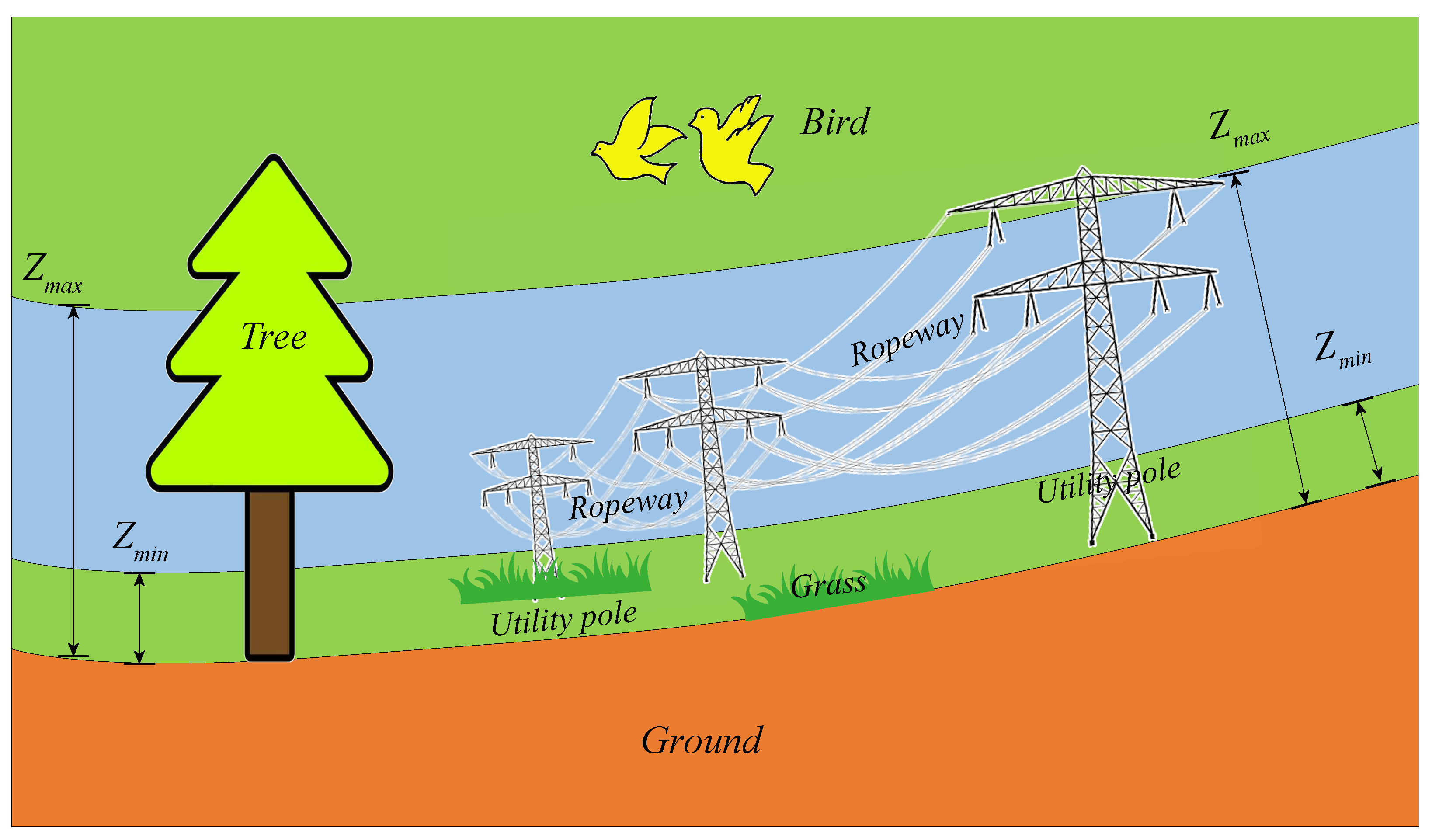
Figure 1. Schematic diagram of the distribution of cables and the surrounding environment ( Z m a x and Z m i n representing the maximum and minimum values of the elevation).
Applsci 13 02875 g001
Figure 2. Diagram of the system’s working principle. In addition, there are different colors in the gradient bar (Applsci 13 02875 i001) in the point cloud data set that represent different altitudes.
Applsci 13 02875 g002
Figure 3. An overview of the elevation filtering process on raw point cloud data: (a) normalized point clouds; (b) elevation-point-figure maps; and (c) elevation filtering effects (white and color).
Applsci 13 02875 g003
Figure 4. There are the front and side views of the first set of sample point clouds (order from left to right): (a) before segmentation and extraction; (b) after preprocessing; (c) after completion of segmentation and extraction; and (d) the comparison display (marked as white and color).
Applsci 13 02875 g004
Figure 5. The front and side of the second set of sample point clouds (order from left to right): (a) before segmentation and extraction; (b) after preprocessing; (c) following segmentation and extraction; (d) displaying the results of the comparison (marked as white and color).
Applsci 13 02875 g005
Figure 6. Views of the third group of sample point clouds from the front and side (order from left to right): (a) before segmentation and extraction; (b) after preprocessing; (c) after segmentation and extraction; (d) the comparison display (marked in white and colored).
Applsci 13 02875 g006
Figure 7. Data analysis chart: (a) represents the proportion of each sample within each group; (b) shows the change in extraction accuracy in each group.
Applsci 13 02875 g007
Figure 8. Processing results of different methods when processing sample data: (a) extraction accuracy; (b) time-consuming.
Applsci 13 02875 g008
Table 1. Models and configuration parameters of software and hardware used in the test experiment.
CategoryConfiguration
SoftwareOperating SystemWin 11
Point-cloud Processing LibraryPCL 1.11.1
Support PlatformVisual Studio 2019
HardwareCPUIntel(R)Core(TM)i5-9400F
MemoryDDR4 32 GB
Graphics CardNvidia GTX 1080 Ti 11 GB
Table 2. The basic situation of each group of test sample data.
Data NameSample NumberNumber of RopewaysNumber of Points
Group One141,018,921
Group Two24485,735
Group Three34557,785
Table 3. Statistical table showing the accuracy rate of ropeway point cloud segmentation and extraction.
Data NameSample NumberNumber of Extracted PointsNumber of Real PointsAccuracy Rate/%
Group One1-11764187394.18
1-21634176692.53
1-31572171191.88
1-44951545290.81
1-all12,02710,80289.81
Group Two2-130332294.10
2-220423885.71
2-324828886.11
2-41573169592.80
2-all2328254391.54
Group Three3-118522681.86
3-234238588.83
3-331132994.53
3-41620177891.11
3-all2458271890.43
Table 4. Accuracy statistics of cable extraction for five groups of samples by different methods (bold indicates the optimal result, underline indicates the suboptimal result, the arrow pointing up indicates that the larger the value is, the better, and the arrow pointing down indicates the smaller the value is, the better).
NameAccuracy Rate/% ↑
RFGBDTSVMVBF-NetOURS
Number-168.5292.8867.7478.3092.52
Number-275.4480.3972.1373.6295.08
Number-376.0967.0843.6665.0583.43
Number-486.3884.2678.5586.8292.18
Number-575.2067.2473.0364.9385.27
Table 5. Time-consuming statistics of cable extraction for five groups of samples by different methods (bold indicates the optimal result, underline indicates the suboptimal result, the arrow pointing up indicates that the larger the value is, the better, and the arrow pointing down indicates the smaller the value is, the better).
NameTime/ms ↓
RFGBDTSVMVBF-NetOURS
Number-154.8155.9273.4945.0128.48
Number-273.2565.6365.3338.6933.25
Number-337.6134.8429.3419.9225.11
Number-487.6270.2267.2083.5342.74
Number-578.2347.5039.4140.6337.29
Disclaimer/Publisher’s Note: The statements, opinions and data contained in all publications are solely those of the individual author(s) and contributor(s) and not of MDPI and/or the editor(s). MDPI and/or the editor(s) disclaim responsibility for any injury to people or property resulting from any ideas, methods, instructions or products referred to in the content.