Flexible Route Planning for Multiple Mobile Robots by Combining Q–Learning and Graph Search Algorithm

Abstract

The use of multiple mobile robots has grown significantly over the past few years in logistics, manufacturing and public services. Conflict–free route planning is one of the major research challenges for such mobile robots. Optimization methods such as graph search algorithms are used extensively to solve route planning problems. Those methods can assure the quality of solutions, however, they are not flexible to deal with unexpected situations. In this article, we propose a flexible route planning method that combines the reinforcement learning algorithm and a graph search algorithm for conflict–free route planning problems for multiple robots. In the proposed method, Q–learning, a reinforcement algorithm, is applied to avoid collisions using off–line learning with a limited state space to reduce the total learning time. Each vehicle independently finds the shortest route using the A* algorithm, and Q–learning is used to avoid collisions. The effectiveness of the proposed method is examined by comparing it with conventional methods in terms of computation time and the quality of solutions. Computational results show that for dynamic transportation problems, the proposed method can generate the solutions with approximately 10% of the computation time compared to the conventional Q–learning approach. We found that the required computation time is linearly increased with respect to the number of vehicles and nodes in the problems.

1. Introduction

Robotics and automation systems have been introduced in recent conveyor systems, warehousing, the food industry, etc. It is necessary to develop automated systems that can make flexible actions to reduce the burden of human work. Automated Guided Vehicles (AGVs) are widely used in large–scale factories such as semiconductor factories, where demands for semiconductor production are increasing. In a transportation system, the task of transporting objects from one initial location to another is given periodically in real–time. The route planning for multiple mobile robots is required to complete the given transportation tasks while avoiding collisions and deadlocks between AGVs and obstacles.

Design and control issues for AGVs have been extensively reviewed in [1,2]. In general, the AGV routing methods are classified as static routing and dynamic routing. Static routing refers to a routing method that provides a conflict–free route according to a start point and a destination point when the set of transportation requests is known in advance. The static routing methods using Dijkstra’s algorithm [3], graph theory [4], iterative neighborhood search [5] and Petri net models [6,7,8] have been proposed. A distributed route planning method for multiple mobile robots using an augmented Lagrangian decomposition and coordination technique has also been proposed [9]. Among them, many graph search–based methods using the A* algorithm [10,11,12,13] or conflict–based search (CBS) [14,15,16,17] have been proposed [18]. In these approaches, the route planning problem is solved by iteratively solving static problems, even in dynamic environments where tasks are given in real–time. However, these approaches have the drawback that it is computationally expensive for solving large–scale problems. If the number of vehicles is increased in a transportation system, the frequency of deadlocks may also increase. It makes it much more difficult to avoid deadlocks and conflicts. A deadlock is a situation in which multiple vehicles are going to the location of another vehicle, and none of the vehicles can travel. Furthermore, unexpected events such as failures or delays may cause collisions that have not appeared in the planning phase.

Therefore, many reinforcement learning methods have been proposed in recent years to solve dynamic routing problems [19]. One of the advantages of using reinforcement learning is that the routing of AGVs can be flexibly regenerated under unexpected situations.

However, reinforcement learning is a trial–and–error method of the searching method to obtain suboptimal solutions. It requires much memory and large–scale computation for trial–and–error. To reduce the computation time, TD (Temporal Difference) learning error [20] is sometimes used to learn Q–values in the Q–learning algorithms. TD learning can reduce the total computation time by allowing AGVs to continuously learn the situations based on the reward obtained after each action. Each AGV determines its action based on the information obtained. Several methods [21,22,23,24] have been proposed for route planning using the Q–learning approach. However, these methods do not ensure the optimality of the solutions, and sometimes, AGV may choose unnecessary actions, which may increase the total traveling time required for transportation.

In this paper, we propose an efficient route planning algorithm that combines Q–learning and a graph search algorithm based on A* algorithm. In the proposed algorithm, the shortest route to the destination of each AGV is searched by the A* algorithm, and Q–learning is used to avoid collisions between AGVs. By combining the A* algorithm with Q–learning, each AGV has the flexibility to accommodate the changes that can cope with unexpected situations, which is an advantage of reinforcement learning, while minimizing the total traveling time, which is an advantage of graph search.

The rest of the paper consists of the following sections. In Section 2, recent research on AGV route planning is presented to clarify the position of this study. In Section 3, the problem description is given, and in Section 4, the details of the proposed method are presented. Section 5, the results of computational experiments are shown, and Section 6 concludes this paper.

2. Related Works

2.1. Classification of Route Planning Problems

There have been many studies on AGV route planning, which can be categorized according to the problem setting under consideration. There are some cases where all transport requirements are initially given to the AGV, as in [25], and cases where transport requirements are given dynamically one after another, as in references [10,26]. While these papers [10,25,26] consider route planning for AGVs in grid space, several approaches have also been proposed for route planning in continuous space [27,28]. As the number of transfer tasks increases, research has also been conducted to help AGVs create task–decision priorities to reduce the total transfer period [29]. The problem set-up varies widely, from those for factory transport [10] to those for AGV use at ports [22,30,31], to those for AGV use at hospitals [32].

There are two main approaches to AGV route planning: one based on optimization methods and the other based on reinforcement learning methods.

2.2. Optimization Methods

Optimization methods are further subdivided into exact, heuristic and search–based algorithms [4]. In exact algorithms, the route planning problem is formulated as an optimization problem, and integer linear programming [33] and Answer–Set Programming [34,35] have been used as solution methods. These methods are applicable in small problem instances to obtain exact solutions [33,35] or suboptimal solutions [36,37,38].

The heuristic algorithm can find a solution to route planning using a series of primitive operations that specify the AGV’s actions in various situations. The optimality of the solution obtained by this approach is not guaranteed. However, it can find a feasible solution in a reasonable time in an environment with many AGVs [39,40].

Popular search–based methods are the conflict–based search (CBS) [14] and A* approaches. One of the difficulties is that the required computation time may increase exponentially with the number of AGVs. CBS is a method that first finds the shortest route for all AGVs ignoring collisions, then adds constraints to avoid collisions. In recent years, many improvement methods have been proposed for CBS, such as ICBS [15] and CBSH [16,17]. Algorithms have also been proposed that use machine learning to learn optimal policies [41] or quasi–optimal policies [42] for search. The same search–based approach has also been proposed for A*–based algorithms [11,12,13].

2.3. Reinforcement Learning Methods

As shown in Table 1, there are many reinforcement learning approaches have been proposed to solve route planning problems [19]. In particular, many Q–learning based algorithms have been proposed [22,31,43,44], and they have better performance in terms of computation time and solution optimality. For example, in [22], the shortest route is found by using Q–learning to estimate the expected waiting time in route planning for AGVs at a port terminal. In [31], Q–learning is performed according to the current position, destination direction, and the number of adjacent vehicles. Ref. [43] utilized the Q–learning to account for the possibility of unexpected delays caused by interference with other vehicles as the vehicle heads toward its destination. Deep reinforcement learning methods have also been used to solve route planning problems for large–scale problem environments. For example, several methods using Deep Q–Network (DQN) have been proposed [45,46,47]. The problem with using DQN is that learning efficiency is reduced due to the slow convergence of the solution. In [46], this problem is remedied by introducing a heuristic reward function. In [47], prior knowledge is combined with DQNs to reduce the learning time. QMix–based method [48] is also helpful. QMix is a type of centralized training with decentralized execution (CTDE), in which action selection is performed in each AGV’s network, and learning is performed using information from all AGVs.

Table 1. Investigated studies using different approaches of reinforcement learning methods.

Authors	Problem	Approach	Real–Time Routing	Continuous Space
Jeon, S.M. et al. [22]	AGVs in port terminals	Q–learning	✓
Lim, J.K. et al. [43]	Multiple AGVs on a grid based network	Q–learning	✓
Sahu, B. et al. [44]	2 actual robots	Q–learning + PSO
Hwang, I. et al. [23]	Semiconductor wafer fabrication facilities	Non–stationary Q–learning	✓
Zhou, P. et al. [31]	Container terminals	Anisotropic Q–learning	✓
Yang, Y. et al. [45]	Multiple AGVs on a grid based network	DQN	✓
Guan, M. et al. [46]	A single AGV on a grid based network	DQN + reward function with heustick	✓
Bae, H. et al. [47]	Multiple AGVs on a grid based network	DQN + prior knowledge	✓
Lou, P. et al. [28]	A single AGVs in continuous space	DQN + prior knowledge	✓	✓
Choi, H.B. et al. [48]	Multiple AGVs on a grid based network	QMIX	✓
Current research	Multiple AGVs on a grid based network	Q–learning + A* algorithm	✓

2.4. Contributions of the Article

Compared with existing approaches, the main contributions of the article can be listed as follows.

• We propose a new route planning algorithm that combines a graph search algorithm and an offline Q–learning algorithm.
• The state space of the proposed Q–learning algorithm is restricted by the integration.
• We found that the optimization performance of the proposed algorithm is almost the same as the conventional route planning algorithms for static problem instances, however, the performance for the dynamic problem is much better than the conventional route planning methods.
• The proposed method can flexibly regenerate route planning dynamically when the delay of AGVs or unexpected events occur.

There has been extensive research on employing Q–learning for AGV route planning, however, no attempt has been made to define the state space based on the relative position of each vehicle. The major originality of the proposed method is that we have developed a new definition of reduced state space in the Q–learning algorithm for solving route planning problems.

3. Problem Description

3.1. Transportation System Model

AGV transportation systems can be classified into unidirectional and bidirectional (see Figure 1). This paper considers bidirectional transport systems with difficult collision avoidance control of AGVs. The transportation system is represented by a graph $G=(V,E)$ where each node $n\in V$ represents a place where only one vehicle can stop, travel, or turn, and each edge $e\in E$ represents a lane where only one vehicle can travel at the same time. A path in G represents the traveling of a vehicle. The following conditions are assumed in the route planning problem.

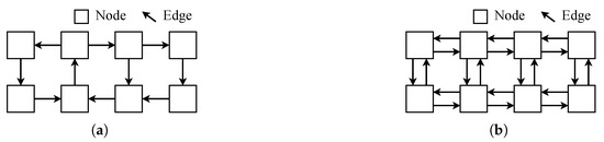
Figure 1. Modeling of AGV transportation systems. AGVs are placed at one of the nodes and can move to adjacent nodes per step. It is not possible for multiple AGVs to be present at the same node at the same time or for two AGVs to move interchangeably between adjacent nodes. (a) Unidirectional transport system. AGVs at a node can only move to the node in the direction of the edge. (b) Bidirectional transport system. AGVs can move to all adjacent nodes if the edges are connected.

• The geometrical size of a vehicle is sufficiently small compared with the size of a node.
• Each vehicle can travel to its adjacent nodes in one unit of time. Therefore, its acceleration and deceleration are not considered.
• A set of an initial node and a destination node represents a transportation task. The time duration defines a task’s transfer period from when the task is loaded at the initial location and is unloaded at the destination location.
• No more than 1 task can be assigned to each vehicle at the same time.
• Loading and unloading time is an integer multiple of one unit time.
• The set of vehicles M and the set of planning periods T are assumed to be constant.
• Conflict on each node and each edge is not allowed.
• The layout of transportation is not changed during the traveling of vehicles.

3.2. Definition of Static Transportation Problem

The static problem is defined as follows. Given a set of transportation tasks and the initial location of vehicles, the objective is to derive conflict–free route planning for multiple vehicles while minimize the total sum of the transfer period of all tasks.

3.3. Definition of Dynamic Transportation Problem

For a dynamic transportation problem, transportation tasks are given in real–time with the progress of the time step. We consider a task queue to hold the set of tasks temporally. The tasks are stored in the task queue. If there is an AGV that has no task, the head of the task queue is assigned to the AGV in the FIFO rule. Each AGV conducts the following steps in the dynamic problem.

• Repeat Steps 2 to 6 until the task queue is empty.
• A task is assigned from the task queue to a waiting AGV which has no task at the time.
• Each AGV travels to the loading location indicated in the task.
• Wait for a certain time at the loading point. (Loading the cargo)
• Travel to the unloading point indicated in the task.
• Wait for a certain time at the unloading point. (Unloading the cargo)

The loading and unloading points are selected from the loading and unloading nodes, respectively. An AGV that is not given a task selects a task from a task queue and generates a route to the loading and unloading points indicated by the task. The transportation time is defined as the time from when the first task is assigned in the task queue to the time when the last task is assigned. In this study, the layout shown in Figure 2 is used for simulation. Each AGV can travel in both directions between nodes connected by edges.

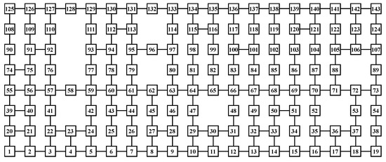
Figure 2. Layout model of a bidirectional transport system with 143 nodes. The squares numbered 1 to 143 represent the nodes that make up the transport system. Each AGV can move to adjacent nodes connected by edges.

3.4. Problem Formulation of Static Problem

The static problem is formulated as an integer programming problem.

3.4.1. Given Parameters

The given parameters are a set of tasks consisting of an initial node $S_{\tau }$ and a destination node $D_{\tau }$ for task $\tau$, the layout of the transportation system $G=(V,E)$, the set of vehicles M, and the set of planning periods T.

3.4.2. Decision Variables

A binary variable $x_{i,j,t}^k\in \{0,1\}$ takes the value of 1 when AGV k travels from node i to node j at time t and 0 otherwise.

3.4.3. Objective Function

The objective function of the route planning problem is to minimize the total transfer period required for transportation. ${\sigma }_{k,\tau }$ is defined as the time period for AGV k to transport the task $\tau$ from initial node $S_{\tau }$ to the destination node $D_{\tau }$. It is represented by 0–1 variable ${\delta }_{k,\tau ,t}$ that takes 1 if AGV k starts from node $S_{\tau }$ until it arrives node $D_{\tau }$, and 0 otherwise. The objective of this problem is to find a conflict–free route for AGVs to minimize the following objective function.

$$\mathrm{minimize}\sum _k\sum _{\tau }{\sigma }_{k,\tau }$$

(1)

The total traveling time ${\sigma }_{k,\tau }$ for AGV k to transport task $\tau$ is represented by the following equations. N is the set of all nodes and $N_i$ is the set of nodes that can be moved from node i.

$$\begin{array}{c}\hfill {\sigma }_{k,\tau }=\sum _{t\in T}{\delta }_{k,\tau ,t}\left(k\in M,t\in T\right)\end{array}$$

(2)

$$\begin{array}{c}\hfill \sum _{i\in N_{S_{\tau }}}{x}_{S_{\tau },i,t}^k\le {\delta }_{k,\tau ,t}\end{array}$$

(3)

$$\begin{array}{c}\hfill {\delta }_{k,\tau ,t}-M\sum _{i\in N_{D_{\tau }}}{x}_{i,D_{\tau },t}^k\le {\delta }_{k,\tau ,t+1}\end{array}$$

(4)

$$\begin{array}{c}\hfill {\delta }_{k,\tau ,t}\le 1-\sum _{i\in N_{D_{\tau }}}{x}_{i,D_{\tau },t}^k\end{array}$$

(5)

Equation (2) defines that the traveling time of task $\tau$ for AGV k is represented by the sum of time counter ${\delta }_{k,\tau ,t}$ which indicates 1 if the traveling is not completed, and 0 otherwise. (3) ensures that once AGV k is started from an initial node, ${\delta }_{k,\tau ,t}$ takes a value of 1. (4) restrict that if AGV k is not arrived at its destination node $D_{\tau }$, ${\delta }_{k,\tau ,t}\le {\delta }_{k,\tau ,t+1}$ is satisfied. ${\delta }_{k,\tau ,t}$ takes the value of 0 once AGV k has arrived at its destination node from (5).

3.4.4. Constraints

The traveling of each AGV satisfies the following constraints. The definition of collision and interference between AGVs in a transportation system is also given below.

$$\sum _{j\notin N_i}{x}_{i,j,t}^k=0\left(k\in M,i\in V\right)$$

(6)

$$\sum _{j\in N_i}{x}_{i,j,t}^k\le 1\left(k\in M,i\in V\right)$$

(7)

$$\sum _{k\in V}\sum _{j\in N}{x}_{j,i,t}^k\le 1\left(i\in V\right)$$

(8)

$$\sum _{k\in V}\left(x_{i,j,t}^k+x_{j,i,t}^k\right)\le 1\left(i\in V,j\in V\right)$$

(9)

Constraints (6) and (7) are obtained from the conditions that AGV k can travel from node i to any node in $N_i$ and that there is only one node where AGV k can exist at any given time t. The constraints on collision avoidance between AGVs and the prohibition of the simultaneous transitions are represented as (8) and (9), respectively.

3.5. Modeling Warehousing System with Obstacles with 256 Nodes and 16 Edges

A warehousing system with obstacles is modeled as a combination of grids. Figure 3 shows an example of a simulation environment that simulates a warehouse. The graph $G(V,E)$ consists of 256 nodes and 16 edges, each in the vertical and horizontal directions, and there are standby and charging nodes, loading nodes, unloading nodes, and obstacle nodes. Standby nodes are the nodes where the locations are not included in the task. Tasks $\tau$ is defined as a pair of one of the loading nodes $S_{\tau }$ and one of the unloading nodes $D_{\tau }$. Each AGV starts for the loading node in the task, waits for 1 time step for loading, and then goes to the unloading node in the task and waits for 1 time step for unloading. If the task queue is not empty, the waiting AGV is given a task again, and each AGV generates its route to the designated loading node. Else, if the task queue is empty, the AGV moves to the waiting node. In the transportation system, six AGVs are utilized as an example. Given a loading node to an unloading node as a task, the task is assigned in turn to the AGVs to which the task has not been assigned. Each AGV $k\in M$ generates its path to minimize the transport path ${\sigma }_{k,\tau }$ while avoiding collisions with each other.

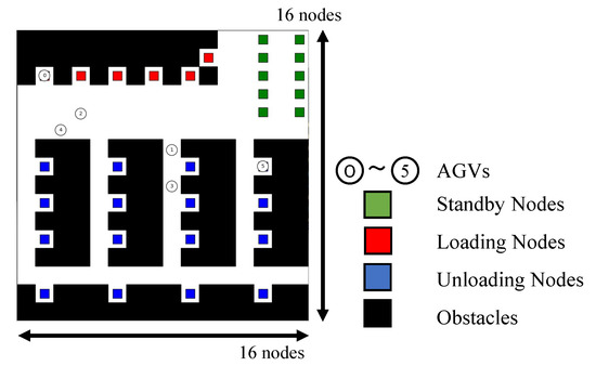
Figure 3. A model of warehousing system with obstacles. Each AGV is initially located at its standby node. Tasks are then assigned to each AGV, which moves to the indicated loading and unloading nodes in that order.

4. Flexible Route Planning Method Combining Q–learning and Graph Search

4.1. Outline of the Proposed Method

A combined method of a graph search algorithm (A* algorithm), and Q–learning, a reinforcement learning method, is applied to solve the route planning problem of multiple AGVs. The framework of the proposed method for the route planning problem of multiple AGVs is shown in Figure 4. After the initial and destination nodes are given to each AGV as a task, each AGV independently generates the shortest path from $S_{\tau }$ to $D_{\tau }$ by using the A* algorithm. If the a possible collision between AGVs is detected, Q–table created by the Q–learning is used to update the actions to avoid the collision. Q–learning is prepared in advance such that AGVs avoid collisions and interference with each other.

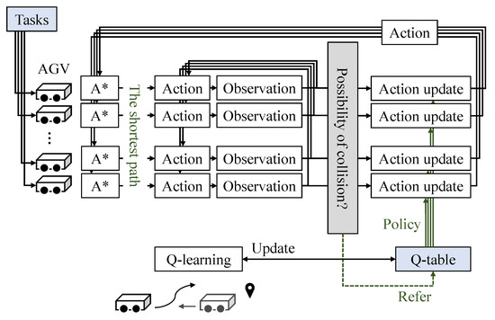
Figure 4. Framework for the proposed method. Each AGV performs A* and Q–learning independently. Collision determination is performed by a central computing system that integrates the positions of all AGVs.

4.2. Combination of A* and Q–learning

4.2.1. A* Search Algorithm

A* algorithm is an algorithm for the graph search problem of finding a path from an initial position to a destination on a graph, using a heuristic function $h\left(n\right)$, which serves as a guidepost for the search. h is a function that returns some reasonable estimate of the distance from each node n to the destination and is solved by various h that can be designed depending on the type of graph search problem. In this paper, the heuristic function is defined as the Manhattan distance between the current position and the destination position. The evaluation value f is the sum of the distance g from the initial position to the current point and the heuristic value h. The priority was determined at random if the evaluation values matched at several nodes.

4.2.2. Q–Learning

Q–learning is an effective method for problems modeled as Markov decision processes. In reinforcement learning, actions that maximize future rewards are learned. If the action value (Q–value), the value of taking action $a_t$ in a certain state $s_t$, is known, the action with the highest Q–value can be selected. In Q–learning, the Q–value is a function that expresses the validity of action a taken in a certain state s based on the policy $\pi$, i.e., the action value function $Q^{\pi }(s,a)$ is expressed by the following expression (10).

$$Q^{\pi }(s_t,a_t)=E_{\pi }\left[\sum _{k=0}^{\infty }{\gamma }^k{r}_{t+k}|s_t=s,a_t=a\right]$$

(10)

Here, r is the reward obtained by the state transition, and $\gamma$ is the discount rate for the reward that is uncertain in the future. The goal of Q–learning is to maximize this action value function $Q^{\pi }(s,a)$. The update of $Q(s,a)$ is performed according to the following (11), which introduces a learning rate $\alpha$.

$$Q(s_t,a_t)+\alpha \left[r_t+\gamma \underset{a^{\prime }}{max}Q(s_{t+1},a^{\prime })-Q(s_t,a_t)\right]$$

(11)

The parameters of the learning rate $\alpha$ and the discount rate $\gamma$ are set to 0.8 and 0.99, respectively.

4.2.3. Definition of State Space

In the conventional Q–learning methods for route planning problems, it is common to use the full transportation system as the state space in Q–learning [49]. However, the learning process is time–consuming due to the increased number of states where a large transportation system is treated. Therefore, in this study, the reduced state space representation is applied. The state s of AGVs used in Q–learning is defined as shown in Figure 5. The state space is defined for each AGV related to the center position of each AGV and is prepared for the number of AGVs. By defining the state space as relatively small compared to the entire transportation system, Q–learning need not be relearned when the number of AGVs increases or when the transportation system is enlarged.

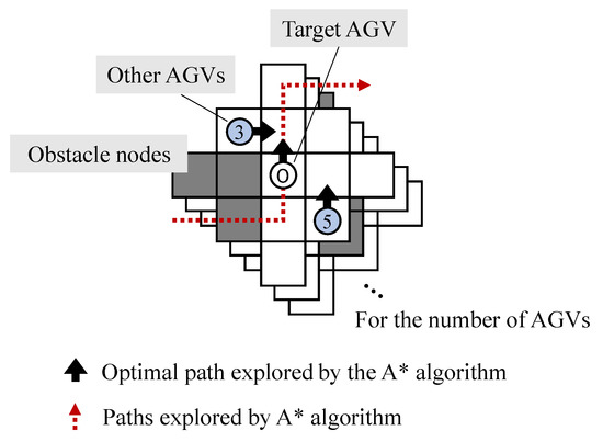
Figure 5. Definition of state space. Each AGV has its own state space centered on its position.

The state space for each AGV is defined as 13 nodes around itself as defined in Figure 5. Each AGV repeats the observation of those nodes in each action step. By adding the path information explored by the A* algorithm to the state space definition and reward setting in Q–learning, we combine the rule–based A* algorithm and Q–learning. The state space in Q–learning is defined for each AGV, which enables the generation of Q–functions that do not require learning again in response to changes in the problem environment or in the number of AGVs. The proposed method does not need to regenerate the plan when any of the motions of AGVs is delayed. It indicates that when unexpected events occur, traffic congestion is avoided for each AGV using the Q–learning, and the impact on the surrounding area is minimized.

There are 4 events to be observed, as shown in Figure 6. First, each AGV detects whether another AGV exists or not for each node. In the example shown in Figure 6, the positions of AGV 1 and AGV 3 are detected. Then, the direction in which it cannot travel in the next state is determined. In the example, the leftward movement is detected as impossible. In addition, the possible interference of other AGVs is determined, and in the example, the potential for interference by moving to the right is detected. Finally, the A* algorithm determines the direction of the explored path. In the example, the direction is determined to be upward.

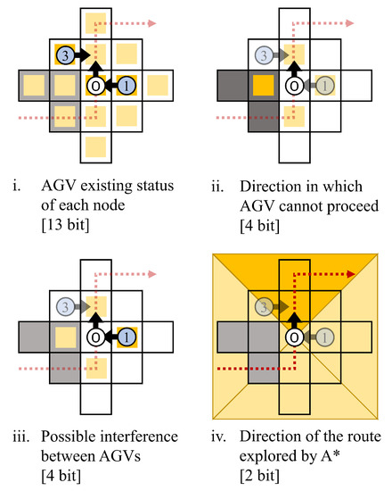
Figure 6. Events to be observed and amount of information. Each event and the amount of information required at that time is shown.

The amount of information for each observed event is given by 13 bits, 4 bits, 4 bits, and 2 bits, respectively, and the number of states of the Q–function is $2^{23}=8,388,608$.

4.2.4. Action Spaces

There are five types of AGV actions: upward, downward, rightward, leftward, and stop. The Q–function is represented by a two-dimensional array of the number of states and the number of actions. In this case, the size of the Q–function is evaluated as $16,777,216\times 5$.

4.2.5. Reward Setting

The reward used for Q–learning $r_t$ is defined as (12), using the path generated by the A* algorithm. The path explored by the A* algorithm is regarded as the shortest path to the destination. Therefore, if it follows the path and does not collide with an obstacle or another AGV, it is highly rewarded. On the other hand, a negative reward is obtained if the AGV chooses an action that results in a collision with an obstacle or another AGV.

$$r_t=\left\{\begin{array}{ccc}2\hfill & if\hfill & {\mathrm{A}}^{*}\mathrm{path}\mathrm{direction}\mathrm{and}\mathrm{forward}\mathrm{action}\hfill \\ 1\hfill & if\hfill & {\mathrm{A}}^{*}\mathrm{path}\mathrm{direction}\mathrm{and}\mathrm{non}\mathrm{forward}\mathrm{action}\hfill \\ 0\hfill & if\hfill & \mathrm{Non}{\mathrm{A}}^{*}\mathrm{path}\mathrm{direction}\mathrm{and}\mathrm{non}\mathrm{stop}\mathrm{action}\hfill \\ -1\hfill & if\hfill & \mathrm{Non}{\mathrm{A}}^{*}\mathrm{path}\mathrm{direction}\mathrm{and}\mathrm{stop}\mathrm{action}\hfill \\ -2\hfill & if\hfill & \mathrm{collision}\mathrm{with}\mathrm{an}\mathrm{obstacle}\mathrm{or}\mathrm{another}\mathrm{AGV}\hfill \end{array}\right.$$

(12)

4.3. Outline of the Proposed Algorithm

The flowchart of the proposed method for solving the route planning problem is shown in Figure 7. First, a Q–function is created offline such that AGVs can learn the actions avoiding collisions and interferences with each other by Q–learning. Then, route planning is conducted. The route planning is implemented by repeating the shortest path search, traveling, state observation, and action updated by the A* algorithm. The details of the route planning algorithm for each AGV are described as follows.

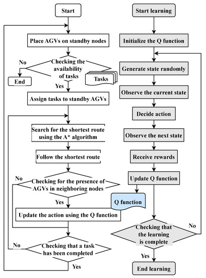
Figure 7. Flowchart of the proposed algorithm. The flowchart on the right side shows the process of building a learning model for Q–learning. The flowchart on the left side shows the process of planning a route using the Q–learning training model that was created.

Step 0  Q–learning

This step generates a Q–function that enables AGVs to avoid collisions. The state space is created randomly, and the rewards are obtained from state observation. Then the action choice is conducted, and the next state is obtained by the action. The process of updating the Q–function using this data is repeated a certain number of times. The Q–function is created only at the first time of route planning. If the Q–function has already been created, the next step is performed.

Step 1  Task assignment

In route planning, a task is first assigned to each AGV. Tasks are assigned to the AGVs that have no task.

Step 2  A* search

Each AGV independently finds the shortest path using A*, regardless of each other’s AGV position.

Step 3  Traveling following the derived path

All AGVs travel along the path explored by the A* algorithm. Simultaneously, all AGVs observe their own state space. If there is another AGV in front of its own state space, it travels to Step 4 due to the possibility of a collision between AGVs. Otherwise, this step is repeated.

Step 4  Update actions

If the possibility of collisions is recognized in the previous step, the action update is performed using the Q–function. In the action update, the state number is derived from the state space observed in the previous step and is referenced to the Q–function. The Q–function returns the action with the highest Q–value, and that action is chosen as the new action. After updating the action, it returns to Step 2 and repeats Step 2 to Step 4 until all AGVs have completed their tasks.

5. Computational Experiments

5.1. Experimental Conditions

Simulation experiments were conducted on a PC with an Intel i5–11400 (2.60 GHz) CPU and 16.0 GB of memory.

5.2. Application to a Small Scale Instance

The initial and final condition for an example problem is shown in Figure 8. Figure 9 shows the route planning by the proposed method. It was confirmed that the proposed method was able to generate a feasible route in a small–scale instance. In the layout with 6 nodes, the routing results of 2 AGVs swapping each other’s position are obtained.

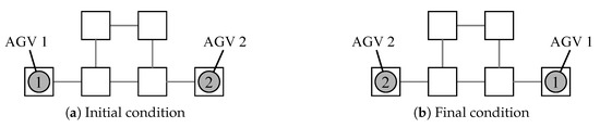
Figure 8. Initial and final condition for a sample route planning problem. Consider the problem of exchanging the positions of AGV1 and AGV2.

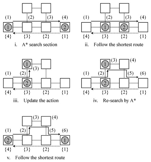
Figure 9. Routing result for two AGVs derived by the proposed method at each iteration. (1), (2), ⋯, (t) indicates the route plan pf AGV1, and 1, 2, ⋯, t indicates the route plan pf AGV2.

First, each AGV independently creates the shortest path to the destination node. The route plans (1), (2), (3), (4) and {1}, {2}, {3}, {4} are tentatively derived. Then, each AGV travels a step at a time along the shortest route it has searched. At this time, AGV 1 cannot travel forward due to the presence of AGV 2 in front. Therefore, an action update occurs, and a new route (1), (2), and (3) is created. After collision avoidance, AGV 1 can generate the shortest route to the destination node by A* again, and feasible route planning (1), (2), (3), (4), (5), and (6) are generated. Finally, each AGV can reach its destination node following the explored route.

5.3. Computational Experiments for Static Problems

5.3.1. Experimental Setup

Our proposed method is compared with the conventional route planning methods in a static problem environment, where all tasks are known. As conventional methods, ADRPM (Autonomous Distributed Route Planning Method) [50] proposed by Ando et al. (2003), and the Q–learning method [49] proposed by Chujo et al. (2020) were utilized. A characteristic feature of ADRPM is that the optimal path is derived when there is no collision or interference between AGVs. Even in the case of collision or interference, a near–optimal path can be generated. By using the method based on Q–learning, the number of deadlocks that occur as the number of AGVs increases can be avoided, and the traveling time can be reduced. In addition, conflict–based search (CBS) [14] was used as the conventional method. The CBS classifies problems into two categories: the high level and the low level. At a high level, a conflict tree is created based on collisions between individual agents. At a low level, a search is performed that satisfies the constraints imposed by the high–level tree structure.

Considering the experiments in a static environment, initial and destination positions are given to each AGV in advance as tasks. The number of AGVs was increased one by one from 1 to 15, and under each condition, the total transfer period taken for all AGVs to complete their tasks and the computation time required for route planning were measured. Here, 10 types of transfer tasks were prepared for each different number of AGVs, and the averages of the 10 repeated experiments for each task were compared. The layout was fixed with a bidirectional transport system consisting of 143 nodes, as shown in Figure 2.

5.3.2. Experimental results

Figure 10 and Figure 11 show the time required for transfer and the computation time required for route planning, respectively, for a comparison of route planning by each method when the number of AGVs is increased. In the route planning by CBS, the computation time became too long when the number of AGVs took larger than 10, and the route could not be found. Figure 10 shows that ADRPM and CBS approaches have the shortest planned path lengths, and the proposed method has longer path lengths than them and also shorter than the method using only Q–learning. When the number of AGVs is small (about 1–3 ), there is no difference in the length of the paths regardless of which method is used. However, as the number of AGVs increases, the difference in the lengths of the paths planned by each method increases.

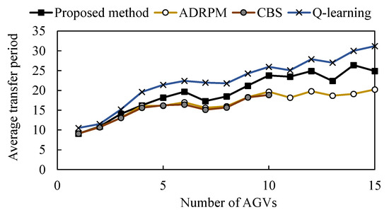
Figure 10. Comparison of total transfer period on static problems. The computation time was measured when the AGV was increased by one unit. For each number of AGVs, 10 initial conditions were prepared, and the average values are shown for each of the 10 experiments conducted under each condition.

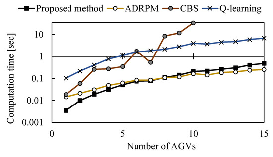
Figure 11. Comparison of computation times on static problems. 10 different initial conditions were prepared at each number of AGVs, and the average of the 10 times under each initial condition was plotted.

Figure 11 shows that the time required for route planning increases with the number of AGVs. For methods other than CBS, the computation time increases linearly with the number of AGVs. In addition, route planning using only Q–learning tended to take longer computation time overall compared to ADRPM and the proposed method. Comparing ADRPM and the proposed method, the change in computation time with the number of AGVs was almost identical, and the proposed method was able to generate routes faster, especially when the number of AGVs was less than 5. The above numerical experiments show the effectiveness of the proposed method in a static problem setting when the number of AGVs is small.

5.3.3. Routing Example

An example of a route obtained by the proposed method is shown in Figure 12. In this example, the number of AGVs is set to 7, and the initial and destination positions of each AGV are shown in Table 2. As shown in Figure 12, each AGV was verified to move toward the destination position while avoiding collisions. AGV1 reached the destination position in only five steps and did not move thereafter, forcing AGV2 to take a long way around. Here, the overall optimization is for AGV1 to stop a few steps just before reaching the destination position and give way to AGV2. This problem arises because the proposed method cannot predict states far into the future from the present.

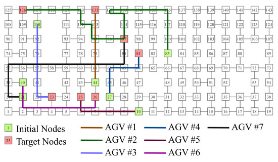
Figure 12. Result of route planning by the proposed method.

Table 2. Initial condition.

AGV	1	2	3	4	5	6	7
Initial node	44	83	110	27	10	40	21
Destination node	131	126	23	81	25	26	97

5.4. Experiments in Dynamic Environments

5.4.1. Experimental Setup

In this section, a comparison of the proposed method and conventional methods is made in a problem environment where tasks are given from time to time. As a conventional method, the approach by Q–learning [49] of Chujo et al. (2020) was used, which can be applied to dynamic problem environments. The number of AGVs was fixed at 10, and given a task from time to time, the total transfer period required to complete a defined number of tasks and the computation time were compared.

5.4.2. Experimental Results

Figure 13 shows the total transfer period required to complete a certain number of tasks, and Figure 14 shows the computation times. Both the proposed method and the approach with only Q–learning increased the total transfer period linearly as the number of tasks increased. The total transfer period to complete 10 tasks is unchanged between the proposed method and the conventional method. However, as the number of tasks increases, the proposed method is able to complete the tasks in a shorter total transfer period. As for the computation time, the proposed method is able to find a path faster, regardless of the number of tasks. These results indicate that the proposed method is effective in a dynamic problem environment where tasks are given from time to time.

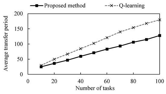
Figure 13. Comparison of total traveling time on dynamic problems.

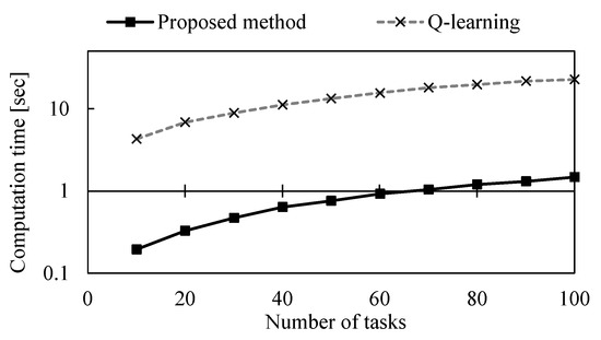
Figure 14. Comparison of computation times on dynamic problems.

5.5. Flexibility of the Proposed Method

A significant feature of the proposed method is that, in an environment where multiple AGVs are operating, it is not necessary to re-plan routes for the entire environment even if some AGVs fail. In the environment shown in Figure 15, 2 AGVs generate their paths to their respective destination points, with the assumption that one of the AGVs slows down in the middle of the path.

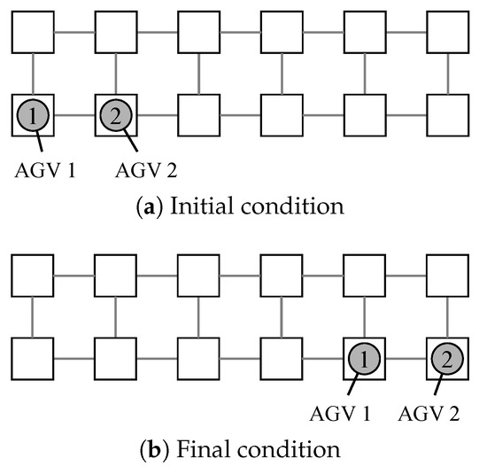
Figure 15. Initial and final condition for a sample route planning problem.

The process routing generated by the proposed method is described (see Figure 16). First, each AGV independently searches for a path to the destination position by A*. Next, AGVs move along the path determined by A* while repeating state observations, while AGV2 slows down in the process. When AGV2 slows down, AGV1 detects it and determines that the traveling along the path of A* would result in a collision. Therefore, AGV1 updates its path in the left direction to avoid collisions by means of the Q–learning model. After avoiding the collision, AGV1 searched again for a path to the destination position by A* and operated according to that path.

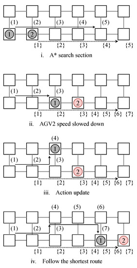
Figure 16. Routing result for two AGVs derived by the proposed method at each iteration. (1), (2), ⋯, (t) indicates the route plan pf AGV1, and 1, 2, ⋯, {t} indicates the route plan of AGV2.

5.6. Computational Efficiency

In this section, the computation time for the proposed method for static problems is evaluated. The calculation time transition was measured as the number of nodes N in the layout or the number of AGVs A increased. The problem environment and initial conditions were randomly generated based on the number of nodes and AGVs in the layout. Route planning with CBS [14] was also performed in the same problem environment for performance evaluation.

Figure 17 shows the transition of calculation time for route planning as the number of nodes N in the layout increases, and Figure 18 shows the transition of computation time as the number of AGVs A increases. Figure 17 shows that the computation time increases linearly with the number of nodes N in the layout. The computational complexity is evaluated as $\mathcal{O}\left(N\right)$. On the other hand, Figure 18 shows that the computation time increases linearly as the number of AGVs A increases. The computational complexity is evaluated as $\mathcal{O}\left(A\right)$. It is superior to CBS, which increases computation time exponentially with the number of nodes N or AGVs A in the layout.

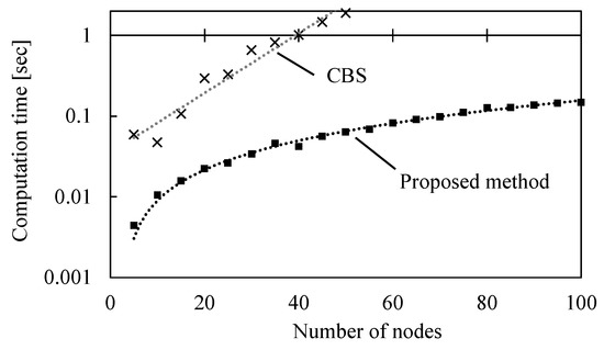
Figure 17. Computation time with respect to the number of nodes N.

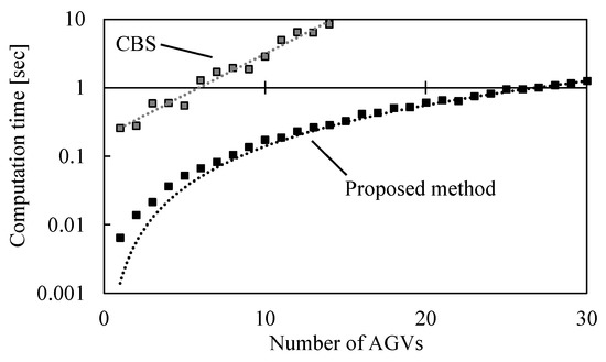
Figure 18. Computation time with respect to the number of AGVs A.

5.7. Impact of Reward Setting

In this section, the impact of the parameter setting of the reward of Q–learning is examined from numerical experiments. AGVs receive higher rewards when choosing actions that follow the path determined by A* and lower rewards when choosing actions that conflict with other AGVs. In addition, other unique reward values are obtained when AGVs choose to move in the direction of their destination or stop (see Equation (12)). When each of these unique reward settings was changed, it was checked how the performance of the proposed method changed. The layout in the experimental environment is shown in Figure 2, where 7 AGVs are given an initial node and a target node, and the transfer period until all AGVs reach the target node is measured. The results are plotted as the average of 10 experiments in the same environment.

Figure 19 shows the transition of the transfer period when each reward parameter is changed. The results show that each reward value can be too low or too high, resulting in poor performance. Therefore, the reward value was selected to reduce the transfer period, as shown in Equation (12).

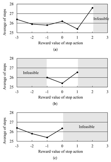
Figure 19. The impact of the parameter setting of the reward of Q–learning. (a) Reward value for A* path direction and non forward action; (b) Reward value for non A* path direction and non stop action; (c) Reward value for non A* path direction and stop action.

6. Conclusions

In this paper, a new route planning method combining a graph search algorithm and a reinforcement learning method was proposed and applied to the AGV route planning problem. A* algorithm was used for the graph search algorithm, and offline Q–learning was used for reinforcement learning. By defining the state space for Q–learning only around each AGV, the model does not need to be re–trained when the layout changes or the number of AGVs changes. This paper clarifies two points. One is that in a problem setting where tasks are given repeatedly, the proposed method can reduce the transfer period and the computation time to approximately 10% of that required to perform route planning using only Q–learning. The second is that the computation time increases linearly with the number of nodes in the layout and with the number of AGVs. This property can help the application of the proposed method in large–scale problems. The reward setting in the proposed method is an important point in the proposed method, and it was clear that route planning will fail if the reward is not set correctly. In terms of directions for future research, it is necessary to add an element of the proposed method to assign tasks appropriately to reduce the transport period in the future. Because only the development of the AGV route planning method has been completed now. It is also necessary to evaluate the proposed method by an experimental system using multiple mobile robots.

References

- Le-Anh, T.; de Koster, M.B.M. A Review of Design and Control of Automated Guided Vehicle Systems. Eur. J. Oper. Res. 2006, 171, 1–23. [Google Scholar] [CrossRef]
- Vis, I.F.A. Survey of Research in the Design and Control of Automated Guided Systems. Eur. J. Oper. Res. 2006, 170, 677–709. [Google Scholar] [CrossRef]
- Dowsland, K.A.; Greaves, A.M. Collision Avoidance in Bi-Directional AGV Systems. J. Oper. Res. Soc. 1994, 45, 817–826. [Google Scholar] [CrossRef]
- Svestka, P.; Overmars, M.H. Coordinated Path Planning for Multiple Robots. Robot. Auton. Syst. 1998, 23, 125–152. [Google Scholar] [CrossRef]
- Ferrari, C.; Pagello, E.; Ota, J.; Arai, T. Multirobot Motion Coordination in Space and Time. Robot. Auton. Syst. 1998, 25, 219–229. [Google Scholar] [CrossRef]
- Dotoli, M.; Fanti, M.P. Coloured Timed Petri Net Model for Real–Time Control of Automated Guided Vehicle Systems. Int. J. Prod. Res. 2004, 42, 1787–1814. [Google Scholar] [CrossRef]
- Nishi, T.; Maeno, R. Petri Net Decomposition Approach to Optimization of Route Planning Problems for AGV Systems. IEEE Trans. Autom. Sci. Eng. 2010, 7, 523–537. [Google Scholar] [CrossRef]
- Nishi, T.; Tanaka, Y. Petri Net Decomposition Approach for Dispatching and Conflict–free Routing of Bidirectional Automated Guided Vehicle Systems. IEEE Trans. Syst. Man Cybern. Part A Syst. Hum. 2012, 42, 1230–1243. [Google Scholar] [CrossRef]
- Nishi, T.; Ando, M.; Konishi, M. Distributed Route Planning for Multiple Mobile Robots Using an Augmented Lagrangian Decomposition and Coordination Technique. IEEE Trans. Robot. 2005, 21, 1191–1200. [Google Scholar] [CrossRef]
- Santos, J.; Rebelo, P.M.; Rocha, L.F.; Costa, P.; Veiga, G. A* Based Routing and Scheduling Modules for Multiple AGVs in an Industrial Scenario. Robotics 2021, 10, 72. [Google Scholar] [CrossRef]
- Standley, T.S. Finding Optimal Solutions to Cooperative Pathfinding Problems. Proc. AAAI Conf. Artif. Intell. 2010, 24, 173–178. [Google Scholar] [CrossRef]
- Goldenberg, M.; Felner, A.; Stern, R.; Sharon, G.; Sturtevant, N.R.; Holte, R.C.; Schaeffer, J. Enhanced partial expansion A*. J. Artif. Intell. Res. 2014, 50, 141–187. [Google Scholar] [CrossRef]
- Wagner, G.; Choset, H. Subdimensional Expansion for Multirobot Path Planning. Artif. Intell. 2015, 219, 1–24. [Google Scholar] [CrossRef]
- Sharon, G.; Stern, R.; Felner, A.; Sturtevant, N.R. Conflict–based Search for Optimal Multi-Agent Pathfinding. Artif. Intell. 2015, 219, 40–66. [Google Scholar] [CrossRef]
- Boyarski, E.; Felner, A.; Stern, R.; Sharon, G.; Tolpin, D.; Betzalel, O.; Shimony, E. ICBS: Improved Conflict–based Search Algorithm for Multi-Agent Pathfinding. Proc. Int. Jt. Conf. Artif. Intell. 2015, 1, 740–746. [Google Scholar] [CrossRef]
- Felner, A.; Li, J.; Boyarski, E.; Ma, H.; Cohen, L.T.; Kumar, K.S.; Koenig, S. Adding Heuristics to Conflict–based Search for Multi-Agent Pathfinding. Proc. Int. Conf. Autom. Plan. Sched. 2018, 28, 83–87. [Google Scholar]
- Li, J.; Boyarski, E.; Felner, A.; Ma, H.; Koenig, S. Improved Heuristics for Multi-Agent Path Finding with Conflict–based Search. Proc. Int. Jt. Conf. Artif. Intell. 2019, 1, 442–449. [Google Scholar]
- Hang, H. Graph–based Multi-Robot Path Finding and Planning. Curr. Robot. Rep. 2022, 3, 77–84. [Google Scholar]
- Yang, E.; Gu, D. Multiagent Reinforcement Learning for Multi-Robot Systems: A Survey; Int. Conf. Control, Autom. Robotics. Vision, Singapore. 2004; Volume 1, pp.1–6. Available online: https://www.researchgate.net/profile/Dongbing-Gu/publication/2948830_Multiagent_Reinforcement_Learning_for_Multi-Robot_Systems_A_Survey/links/53f5ac820cf2fceacc6f4f1a/Multiagent-Reinforcement-Learning-for-Multi-Robot-Systems-A-Survey.pdf (accessed on 22 January 2023).
- Boyan, J.A. Technical Update: Least-Squares Temporal Difference Learning. Mach. Learn. 2002, 49, 233–246. [Google Scholar] [CrossRef]
- Bai, Y.; Ding, X.; Hu, D.; Jiang, Y. Research on Dynamic Path Planning of Multi-AGVs Based on Reinforcement Learning. Appl. Sci. 2022, 12, 8166. [Google Scholar] [CrossRef]
- Jeon, S.; Kim, K.; Kopfer, H. Routing Automated Guided Vehicles in Container Terminals Through the Q–learning Technique. Logist. Res. 2011, 3, 19–27. [Google Scholar] [CrossRef]
- Hwang, I.; Jang, Y.J. Q (λ) Learning–based Dynamic Route Guidance Algorithm for Overhead Hoist Transport Systems in Semiconductor Fabs. Int. J. Prod. Res. 2019, 58, 1–23. [Google Scholar] [CrossRef]
- Watanabe, M.; Furukawa, M.; Kinoshita, M.; Kakazu, Y. Acquisition of Efficient Transportation Knowledge by Q–learning for Multiple Autonomous AGVs and Their Transportation Simulation. J. Jpn. Soc. Precis. Eng. 2001, 67, 1609–1614. [Google Scholar] [CrossRef]
- Eda, S.; Nishi, T.; Mariyama, T.; Kataoka, S.; Shoda, K.; Matsumura, K. Petri Net Decomposition Approach for Bi-Objective Routing for AGV Systems Minimizing Total Traveling Time and Equalizing Delivery time. J. Adv. Mech. Des. Syst. Manuf. 2012, 6, 672–686. [Google Scholar] [CrossRef][Green Version]
- Umar, U.A.; Ariffin, M.K.A.; Ismail, N.; Tang, S.H. Hybrid multiobjective genetic algorithms for integrated dynamic scheduling and routing of jobs and automated-guided vehicle (AGV) in flexible manufacturing systems (FMS) environment. Int. J. Adv. Manuf. Technol. 2015, 81, 2123–2141. [Google Scholar] [CrossRef]
- Duinkerken, M.B.; van der Zee, M.; Lodewijks, G. Dynamic Free Range Routing for Automated Guided Vehicles. In Proceedings of the 2006 IEEE International Conference on Networking, Sensing and Control, Ft. Lauderdale, FL, USA, 23–25 April 2006; pp. 312–317.
- Lou, P.; Xu, K.; Jiang, X.; Xiao, Z.; Yan, J. Path Planning in an Unknown Environment Based on Deep Reinforcement Learning with Prior Knowledge. J. Intell. Fuzzy Syst. 2021, 41, 5773–5789. [Google Scholar] [CrossRef]
- Qiu, L.; Hsu, W.J.; Huang, S.Y.; Wang, H. Scheduling and Routing Algorithms for AGVs: A Survey. Int. J. Prod. Res. 2002, 40, 745–760. [Google Scholar] [CrossRef]
- Liang, C.; Zhang, Y.; Dong, L. A Three Stage Optimal Scheduling Algorithm for AGV Route Planning Considering Collision Avoidance under Speed Control Strategy. Mathematics 2023, 11, 138. [Google Scholar] [CrossRef]
- Zhou, P.; Lin, L.; Kim, K.H. Anisotropic Q–learning and Waiting Estimation Based Real–Time Routing for Automated Guided Vehicles at Container Terminals. J. Heuristics 2021, 1, 1–22. [Google Scholar] [CrossRef]
- Pedan, M.; Gregor, M.; Plinta, D. Implementation of Automated Guided Vehicle System in Healthcare Facility. Procedia Eng. 2017, 192, 665–670. [Google Scholar] [CrossRef]
- Yu, J.; LaValle, S.M. Optimal Multirobot Path Planning on Graphs: Complete Algorithms and Effective Heuristics. IEEE Trans. Robot. 2016, 32, 1163–1177. [Google Scholar] [CrossRef]
- Erdem, E.; Kisa, D.G.; Oztok, U.; Schueller, P. A General Formal Framework for Pathfinding Problems with Multiple Agents. In Proceedings of the AAAI Conference on Artificial Intelligence, Bellevue, WA, USA, 14–18 July 2013; pp. 290–296. [Google Scholar]
- Gómez, R.N.; Hernández, C.; Baier, J.A. Solving Sum-Of-Costs Multi-Agent Pathfinding with Answer-Set Programming. AAAI Conf. Artif. Intell. 2020, 34, 9867–9874. [Google Scholar] [CrossRef]
- Surynek, P. Reduced Time-Expansion Graphs and Goal Decomposition for Solving Cooperative Path Finding Sub-Optimally. Int. Jt. Conf. Artif. Intell. 2015, 1916–1922. [Google Scholar]
- Wang, J.; Li, J.; Ma, H.; Koenig, S.; Kumar, T.K.S. A New Constraint Satisfaction Perspective on Multi-Agent Path Finding: Preliminary Results. In Proceedings of the International Conference on Autonomous Agents and Multiagent Systems, Montreal, QC, Canada, 13–17 May 2019; pp. 417–423. [Google Scholar]
- Han, S.D.; Yu, J. Integer Programming as a General Solution Methodology for Path–based Optimization in Robotics: Principles, Best Practices, and Applications. In Proceedings of the International Conference on Intelligent Robots and Systems, Macau, China, 3–8 November 2019; pp. 1890–1897. [Google Scholar]
- Luna, R.; Bekris, K.E. Push and Swap: Fast Cooperative Path-Finding with Completeness Guarantees. In Proceedings of the International Joint Conference on Artificial Intelligence, San Francisco, CA, USA, 7–11 August 2011; pp. 294–300. [Google Scholar]
- Sajid, Q.; Luna, R.K.; Bekris, E. Multi-Agent Pathfinding with Simultaneous Execution of Single-Agent Primitives. In Proceedings of the 5th Annual Symposium on Combinatorial Search, Niagara Falls, ON, Canada, 19–21 July 2012; pp. 88–96. [Google Scholar]
- Huang, T.; Koenig, S.; Dilkina, B. Learning to Resolve Conflicts for Multi-Agent Path Finding with Conflict–based Search. Proc. Aaai Conf. Artif. Intell. 2021, 35, 11246–11253. [Google Scholar] [CrossRef]
- Huang, T.; Dilkina, B.; Koenig, S. Learning Node-Selection Strategies in Bounded-Suboptimal Conflict–based Search for Multi-Agent Path Finding. In Proceedings of the International Joint Conference on Autonomous Agents and Multiagent Systems, Virtual Conference, Online, 3–7 May 2021; pp. 611–619. [Google Scholar]
- Lim, J.K.; Kim, K.H.; Lim, J.M.; Yoshimoto, K.; Takahashi, T. Routing Automated Guided Vehicles Using Q–learning. J. Jpn. Ind. Manag. Assoc. 2003, 54, 1–10. [Google Scholar]
- Sahu, B.; Kumar Das, P.; Kabat, M.R. Multi-Robot Cooperation and Path Planning for Stick Transporting Using Improved Q–learning and Democratic Robotics PSO. J. Comput. Sci. 2022, 60, 101637. [Google Scholar] [CrossRef]
- Yang, Y.; Li, J.; Peng, L. Multi-robot path planning based on a deep reinforcement learning DQN algorithm. CAAI Trans. Intell. Technol. 2020, 5, 177–183. [Google Scholar] [CrossRef]
- Guan, M.; Yang, F.X.; Jiao J., C.; Chen, X.P. Research on Path Planning of Mobile Robot Based on Improved Deep Q Network. J. Phys. Conf. Ser. 2021, 1820, 012024. [Google Scholar] [CrossRef]
- Bae, H.; Kim, G.; Kim, J.; Qian, D.; Lee, S. Multi-Robot Path Planning Method Using Reinforcement Learning. Appl. Sci. 2019, 9, 3057. [Google Scholar] [CrossRef]
- Choi, H.B.; Kim, J.B.; Han, Y.H.; Oh, S.W.; Kim, K. MARL–based Cooperative Multi-AGV Control in Warehouse Systems. IEEE Access 2022, 10, 100478–100488. [Google Scholar] [CrossRef]
- Chujo, T.; Nishida, K.; Nishi, T. A Conflict–free Routing Method for Automated Guided Vehicles Using Reinforcement Learning. In Proceedings of the International Symposium on Flexible Automation, Virtual Conference, Online, 8–9 July 2020. Paper No. ISFA2020-9620. [Google Scholar]
- Ando, M.; Nishi, T.; Konishi, M.; Imai, J. An Autonomous Distributed Route Planning Method for Multiple Mobile Robots. Trans. Soc. Instrum. Control. Eng. 2003, 39, 759–766. [Google Scholar] [CrossRef]
Disclaimer/Publisher’s Note: The statements, opinions and data contained in all publications are solely those of the individual author(s) and contributor(s) and not of MDPI and/or the editor(s). MDPI and/or the editor(s) disclaim responsibility for any injury to people or property resulting from any ideas, methods, instructions or products referred to in the content. |
© 2023 by the authors. Licensee MDPI, Basel, Switzerland. This article is an open access article distributed under the terms and conditions of the Creative Commons Attribution (CC BY) license (https://creativecommons.org/licenses/by/4.0/).