Abstract
Due to the complex terrain and intense tectonic activity, and harsh climate in the Qinling-Daba Mountains, many landslides occur in the area. Most of these landslides are extremely active, posing a serious threat to the safety and property of local residents. As a mature deformation-monitoring technology, InSAR has been widely used in landslide detection, but the steep terrain and dense vegetation in the Qinling-Daba Mountains make detection challenging. Hence, it is important to choose suitable data sources and methods for landslide detection via InSAR in this area. This study was the first to collect ALOS/PALSAR−2 and Sentinel−1A images to detect landslides in the Qinling-Daba Mountains, applying a method combining IPTA and SBAS. In total, 88 landslides were detected and validated. The results show that the deformation-detection error rate of Sentinel−1A is 2% higher than that of ALOS/PALSAR−2 and that its landslide-recognition rate is 47.7% lower than that of ALOS/PALSAR−2. Upon comparing and analyzing the visibility, coherence, closed−loop residuals, and typical time series of landslide deformation from the two kinds of data, it was found that the extremely low quality of available Sentinel−1 A summer data is a major factor influencing that system’s performance. ALOS/PALSAR−2 is more likely to detect landslides in areas with high vegetation coverage, meeting more than 90% of the monitoring needs. It is thus highly suitable for landslide detection in the Qinling–Daba Mountains, where seasonality is significant. In this paper, for the first time, multiple data sources are compared in detail with regard to their utility in landslide detection in the Qinling–Daba Mountains. A large number of accuracy metrics are applied, and the results are analyzed. The study provides important scientific support for the selection of data sources for future landslide monitoring in the Qinling–Daba Mountain area and similar areas and for the selection of methods to evaluate the accuracy of InSAR monitoring.
1. Introduction
Mountainous areas can be complex and dangerous, characterized by high mountains and deep valleys, complex and changeable stratigraphic lithologies, complex geological structures, high vegetation coverage, and harsh and changeable climates. These areas bring considerable difficulty to the identification of geological disasters. As is typical of complex and dangerous mountainous areas, the Qinling-Daba Mountains have steep terrain, high vegetation coverage, complex lithology, and mountains and hills [1,2]. The distinctive terrain and local hydrological cycle make the rainfall in this area short-lived, strong and frequent [3]. In recent years, human engineering activities such as building railways, highways, and houses have gradually increased in frequency in the area. These activities have reduced vegetation and reduced slope stability. As a result, the rate of geological disasters, especially landslides, is increasing in the region. Therefore, the selection of appropriate and effective landslide-detection methods will be of great significance for the detection of geohazards in the Qinling-Daba Mountains and other similar areas.
Due to the wide range of research areas, harsh environments, and complex terrains, it is difficult to monitor mountainous regions using traditional artificial and ground−based disaster−identification methods. Since Graham first proposed the use of synthetic aperture radar interferometry technology (InSAR) to monitor small surface deformations in 1974 [4], the advantages of this technology has been demonstrated. These advantages include being independent of time and climate and having the ability to detect deformation with a high level of precision. Today, this technology is widely used in the early detection of landslides, debris flows, collapses, and other geological disasters over a large range [5,6,7]. InSAR technology used for geohazard monitoring can achieve millimeter−level accuracy, and good progress has been made [8,9,10].
In terms of data sources, there are several SAR satellites of different bands currently in orbit, including Sentinel−1A and Radarsat−2 in C−band, COSMO−SkyMed, TerraSAR−X in X−band, ALOS/PALSAR−2, SAOCOM, and L−SAR in L−band, etc. Each radar wavelength has its own penetration performance and accuracy in deformation monitoring; for example, long-wave radar has good penetration performance to ground objects at the cost of slightly lower deformation accuracy, while short-wave radar has higher deformation accuracy at the cost of weaker penetration performance. Each satellite has different characteristics. Free C−band Sentinel−1A/B data and L−band ALOS−2 data are two kinds of data with excellent performance and have become the leaders in radar data. Therefore, it is particularly important to consider the geological history and landslide characteristics of different regions in selecting the monitoring data most suitable to the region.
To date, a large number of scholars have used SBAS−InSAR, PS−InSAR, and D−InSAR technology to detect potential geohazards in complex and dangerous mountainous areas and have obtained good monitoring results [11,12,13,14], indicating that InSAR technology has substantial advantages in monitoring potential geohazards. Most of the work carried out in the Qinling-Daba Mountains is focused on geological mechanisms and characteristics [15,16,17,18,19]. Some scholars have also detected and studied typical geological hazards in the Qinling–Daba Mountains based on InSAR technology and analyzed the principles of their movement and the factors that induce movement. Study areas have included the Bailong River Basin [20,21], the Jiangdingya landslide [22], and typical landslides in Lueyang County [23], with studies reaching a shared, clear understanding of the typical landslides in the region. Some scholars have also used a variety of data types to jointly identify areas with high concentrations of potential geohazards or single geohazards in complex and dangerous mountainous areas and analyzed the recognition effect [24,25,26,27,28], providing a foundation for subsequent scholars to use in choosing appropriate data for monitoring and research analysis. However, most of these studies examine alpine canyons and karst areas. There is little research examining the type of landslides seen in the Qinling–Daba Mountains, which are small in scale and mostly shallow. Therefore, it is necessary to use different data to detect landslides in such areas and analyze their adaptability.Considering this issue, we took as an example Ankang, which is a typical area in the Qinling-Daba Mountains. We collected 19 Sentinel−1A and 10 ALOS/PALSAR−2 images and utilized time-series radar technology to analyze the potential for landslides in the study area. Various spatial and clustering statistical methods were adopted for the comparison and analysis of the two data sources. The potential for adapting the two data types to monitoring in the region was evaluated, and a method for landslide detection is given here. This method provides effective support for the selection of data sources to detect geological disasters and the implementation of monitoring in the Qinling–Daba Mountains.
2. Study Area and Data
2.1. Study Area
The Qinling–Daba Mountains in southern Shaanxi are located between 105°29′~111°2′ E and 31°42′~34°26′ N (Figure 1). The altitude is mostly in the range of 1000~3000 m [29]. In addition to the high mountains, basins and valleys formed due to the subsidence of the block [30]. These features include the Hanzhong Basin, Ankang Basin, Hanying Basin, and Xixiang Basin [31]. The Qinling-Daba Mountains span the Qinling, Northern China, and Yangzi plates and include widely distributed metamorphic rocks such as slate, phyllite, and schist, with a weak lithology. The lithological joints and fissures are well developed and strongly weathered, which is highly conducive to the occurrence of geohazards [32]. These mountains constitute an important boundary between northern and southern China, and there are significant differences in climate and rainfall between the northern and southern parts of the Qinling–Daba Mountains. The southern part belongs to the subtropical monsoon climate zone, while the northern part belongs to the temperate monsoon climate zone. The airflow enters a strong sinking area after crossing the Qinling-Daba Mountains, and the precipitation decreases sharply at that point. Due to the significant difference in terrain, there are also obvious vertical zonal climate characteristics [33]. The northern part has abundant rainfall at an altitude of 1000~1400 m. In the southern area, there is also high rainfall, and rainstorms and continuous rainfall are common due to the influence of the uplift and blocking of the airflow below 1000 m above sea level. These factors result in the frequent occurrence of geological disasters in the rainy season. Restricted by geological and geomorphological conditions, landslides are mainly shallow and small or medium-sized, and they can be mainly divided into soil and rock types according to material composition [33]. These landslides mainly occur from July to October and are strongly related to rainfall factors [34]. Landslides in the region are often interrelated in terms of causes and interdependent in time and space [35], showing regional aggregation. Such trends have been observed in the Ziyang-Hongshan landslide group, the Heihe-Ganyuwan landslide group, the Ziyang-Gaoping landslide group, etc. Ankang, as a typical disaster-vulnerable area in the Qinling-Daba Mountains, is a representative example [35]. Therefore, the authors of this paper chose Ankang as a site in which to explore the adaptability of Sentinel−1A and ALOS/PALSAR−2 data.
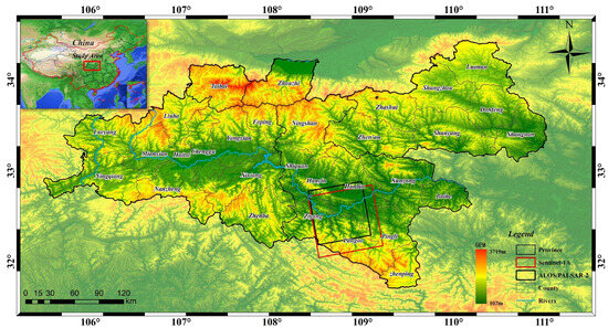
Figure 1.
The Qinling-Daba Mountains and study area.
2.2. Data
As short-wave and long-wave SAR data sources, Sentinel−1A and ALOS/PALSAR−2 have stable satellite flight and excellent performance in obtaining deformation time-series data. They represent the most commonly used radar-satellite data. Therefore, these two mainstream data types were chosen for comparison and analysis of their adaptability to use in landslide monitoring.
In 2014, the ESA launched the environmental observation satellite Sentinel−1A and implemented a policy of free and open use. This satellite is equipped with a C−band (5.6 cm) sensor and uses a new terrain-observation method with progression scans (TOPS) imaging technology [36]. Its short revisit period (12 days), wide coverage, rich collection of archived and open-access data, and sensitivity to surface deformation have made it an important data source for monitoring of deformations such as landslides and earthquakes. However, it still has some disadvantages, such as its low resolution and weak penetration [37,38]. ALOS−2 is a land-observing satellite equipped with SAR sensors that was launched by Japan’s JAXA in 2014. It has three types of imaging: strip, spotlight, and wide-mode. The radar sensor PALSAR (Phased Array type L−band Synthetic Aperture Radar) has a wavelength in the L−band that has better penetrating ability than other short-band sensors [36], and its performance is significantly better than that of ALOS−1. The radar images have high spatial resolution, and richer information can be obtained in mountainous areas [39,40], making this sensor suitable for resource investigation, geohazard monitoring and mapping, etc.
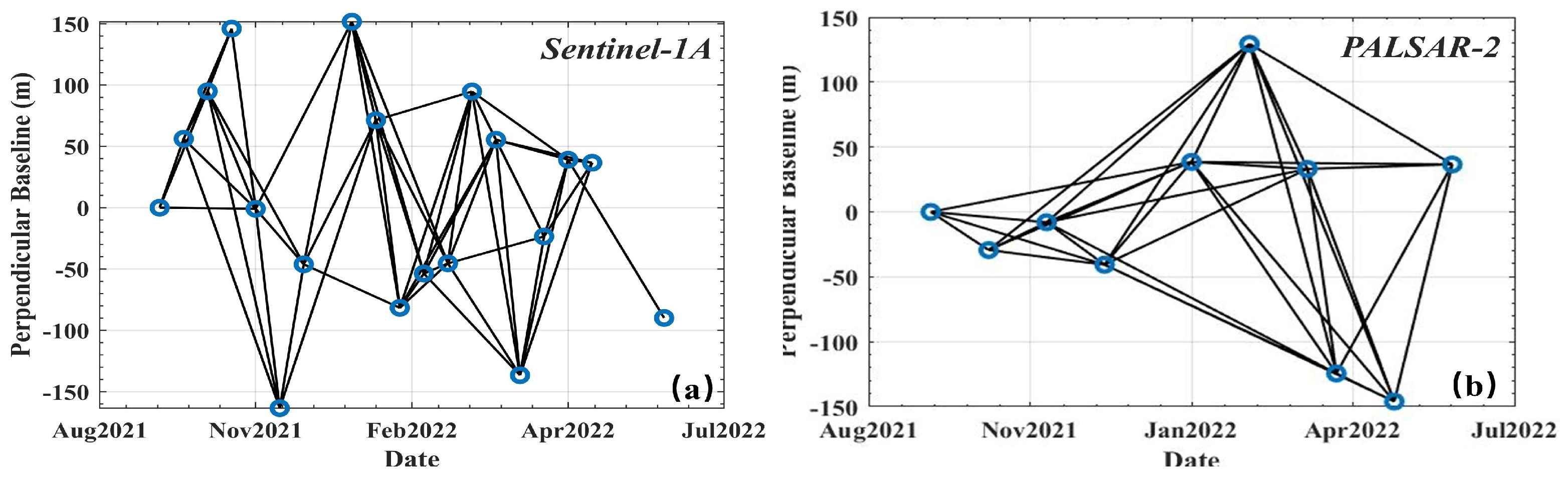
In this paper, the coverage areas of Sentinel−1A and ALOS/PALSAR−2 are clipped (Figure 1) to compare the potential of the two data sources to be adapted for use in landslide detection. The main parameters of the two satellite sensors and the details of the images used in this experiment are shown in Table 1 and Table 2. For distributed backscattering points, the longer the baseline, the lower the coherence. Therefore, it is particularly important to set the appropriate baseline threshold. The Sentinel−1A data have poor penetration and a short revisit period, while the ALOS/PALSAR−2 data are the opposite. To combine these data characteristics and ensure that sufficient interference pairs can be obtained, we set the temporal and spatial baselines of the Sentinel−1A to 48 days and ±150 and the temporal and spatial baselines of ALOS/PALSAR−2 are set to 140 days and ±150. Finally, 55 and 33 interference pairs were generated, respectively (Figure 2).

Table 1.
The parameters of Sentinel−1A and ALOS/PALSAR−2 sensors.
Table 2.
Basic description of the SAR data used herein.
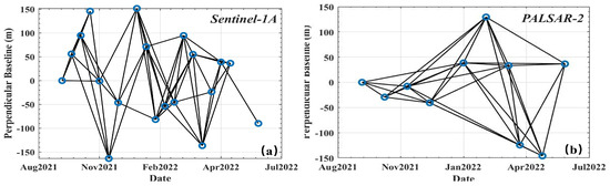
Figure 2.
Temporal and spatial baseline diagrams. (a) Sentinel−1A, (b) PALSAR−2. The blue circle represents the temporal position and spatial relative position of the image.
3. Methods
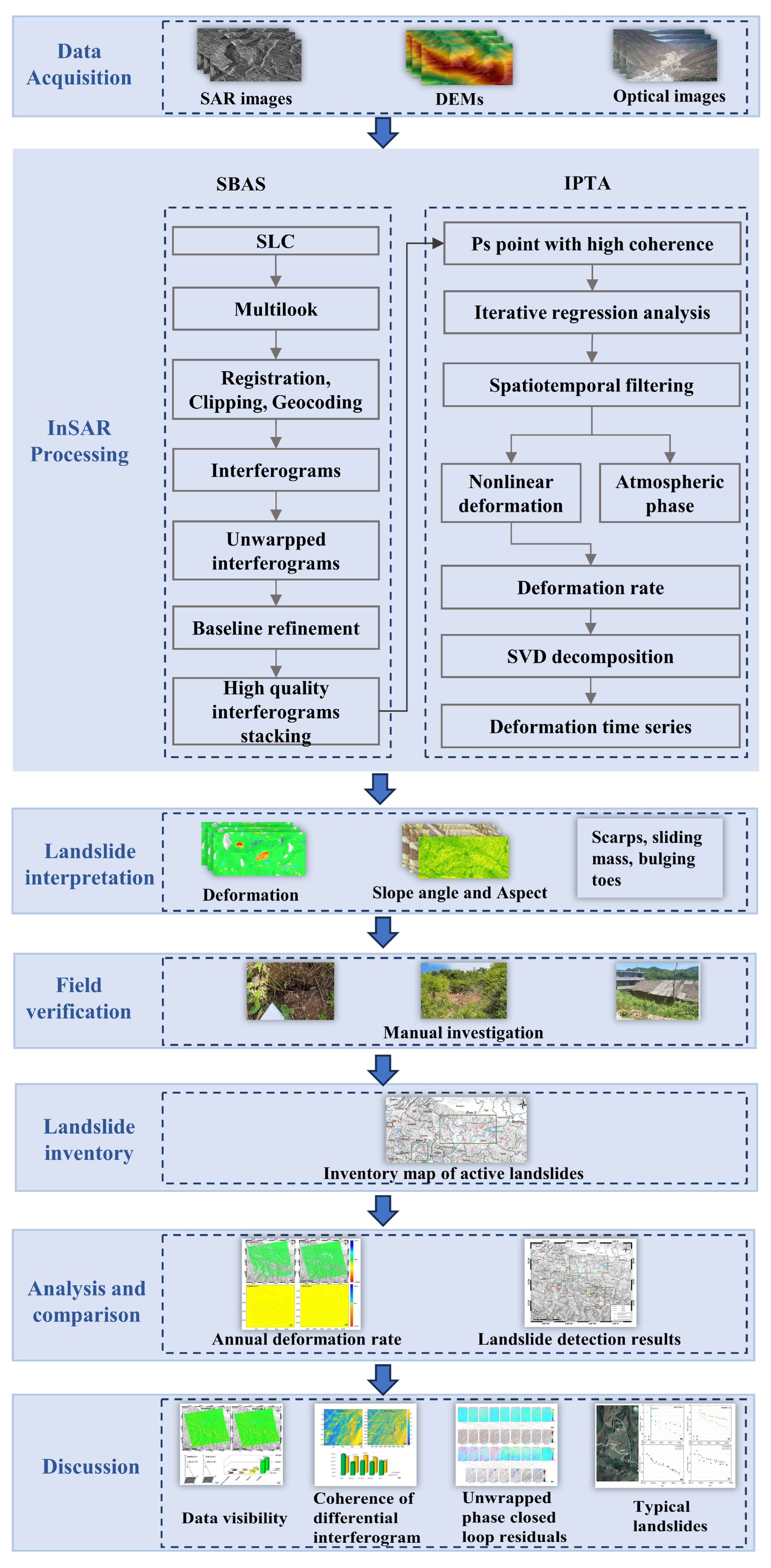
SBAS−InSAR [41] and PS−InSAR [42] have become the most commonly used technologies for obtaining deformation time-series data and have achieved very good results in the monitoring of many landslides. Therefore, this paper combines SBAS−InSAR and IPTA [43] technology developed based on PS−InSAR and leverages the advantages of the free combination of interference pairs in SBAS and the iterative characteristics of IPTA to obtain continuous, high-precision deformation data. Then, the results are superimposed on DEM and optical images for landslide detection. In this paper, SRTM DEM with a resolution of 30 m is used as DEM data and Google Earth images with an approximate resolution of 0.5 m are used for optical data. The DEM data are used to determine the slope of the terrain; usually, areas with a slope of less than 10° are considered free of landslides. During the InSAR monitoring period, only some areas of slopes will undergo obvious deformation. It is thus difficult to fully characterize the entire landslide only from the InSAR deformation results. Hence, it is necessary to utilize the auxiliary optical images for better detection [44,45]. Based on the high-precision landslide-identification/monitoring system, this paper uses Sentinel−1A and ALOS/PALSAR−2 as data sources to detect landslides and compares the differences between the two data types in terms of deformation rate and recognition. Further, this investigation explores the reasons for the differences between the two data sources by calculating the visibility, the coherence of the interference pairs, the quality of unwrapped images, and the rate and time-series results for single landslide points. Finally, the overall adaptability of the two data types and suggestions for future landslide-detection methods are summarized. The specific technical process of landslide detection and analysis is shown in Figure 3.
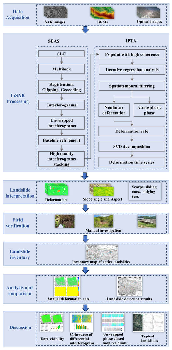
Figure 3.
Flowchart for the detection of potential landslides in the Qinling-Daba Mountains.
3.1. SBAS−IPTA
SBAS is a differential interferometry method proposed by Berardino [46] that can efficiently obtain continuous deformation data. It first divides all SAR images into short baseline subsets according to temporal and spatial baselines and then performs interferometry on a single subset. The minimum cost flow unwrapping method is used to perform phase unwrapping, and the observation equation is established with high-coherence points. Finally, the singular value decomposition (SVD) [47] method is used to obtain the minimum norm solution of the velocity vector. The integral can obtain the deformation over each time period. It uses multiple master images to reduce the amount of SAR data required and can effectively weaken the influence of decoherence and topographic changes by controlling the temporal and spatial baselines [48].
The IPTA processing module designed by Werner in Gamma software (https://www.gamma-rs.ch/, accessed on 10 October 2023) can independently set up multiple master images or a single master image and reduce the error interference via regression analysis and multiple iterations to obtain surface deformation [43]. The basic idea is to select a target point with stable backscattering characteristics and obtain the linear deformation, DEM difference, and residual of the target point via one-dimensional or two-dimensional regression analysis. After the DEM error is corrected, the atmospheric delay in the residual is separated from the nonlinear deformation by time–space domain filtering, so that the deformation time-series data of each target point can be obtained. This technique gradually weakens the interference of decoherence noise, atmospheric delay, and DEM error in the results through multiple iterations [43,49]. Unlike SBAS, IPTA only performs interference processing and time-series analysis on permanent scatterer targets with high-coherence points and cannot obtain the complete range and shape of landslides. Therefore, when SBAS and IPTA technologies are combined, they can learn from each other and obtain more accurate results for continuous deformation. Both of these methods are relatively mature at present, and their specific theories will not be described in this paper.
The specific processing flow of SBAS−IPTA is as follows:
- Select the master image and resample the slave image into the master image space; the master image will try to select the image with less vegetation coverage and the date in the middle.
- According to the imaging quality and quantity of different images, set an appropriate threshold temporal and spatial baselines for differential interference; combine external DEM data to remove the terrain phase of the interferometric phase.
- Use the adaptive filtering method to filter the interference image; the filtering window is usually 32 or 64.
- Use the minimum cost flow (MCF) method for phase unwrapping [50].
- Select high-quality interferometry pairs and perform baseline refinement, re-interferometry, filtering, unwrapping, etc.
- Select permanent scatterer points (PS) with high coherence and obtain a set of differential interference points [51];
- Select a stable reference point (usually buildings) for iterative regression analysis; decompose the deformation phase, elevation correction phase, and residual phase; and iterate until there is no obvious phase jump in the residual phase.
- Separate the atmospheric error phase from the residual phase by using the spatial-temporal domain filtering method.
- Establish an observation equation using the acquired high-coherence points and use singular-value decomposition (SVD) to obtain the deformation rate and time-series results [47].
3.2. Hot-Spot Analysis
Generally, the most reliable deformation-area data in the monitoring results obtained by SBAS−IPTA do not appear as single deformation points. Instead, there are obvious clusters of low or high values. In contrast, errors are usually distributed discretely and randomly across the results [52]. Hotspot analysis is usually used to judge whether spatial values have clustering properties. Therefore, this paper uses hotspot analysis to identify the effective deformation and error areas in the deformation rate. It is important to determine the appropriate distance for spatial analysis. In this paper, the spatial incremental auto-correlation analysis is used to determine the optimal analysis distance [53]. The whole process is based on the Global Moran’s statistic, which calculates the z-score of the feature at different distances and finally uses the z-value peak as the distance threshold parameter of the spatial analysis. The equation is as follows:
where n is the total number of elements when performing spatial clustering, is the average value of all elements, is the spatial weight of the element, and is the sum of all spatial weights. The formula is as follows:
From the results of Global Moran’s I index, the z-value is used to determine the degree of spatial auto-correlation, which is calculated as follows:
where the calculation of E[I] and Var[I] is as follows:
After the optimal distance threshold is obtained, the statistical model can be used to see whether the monitoring feature points within a certain distance have significant spatial clustering:
where n is the total number of elements, is the total number of elements within the distance threshold, is the deformation value, and is the average value of the elements. The Getis–Ord statistics for each element are represented by their z-value and p-value. The p-value is the significance level in the hypothesis test [54]. The z-value indicates the statistical significance of the clustering at the 90% (p value 0.10), 95% (p value 0.05), and 99% (p value 0.01) confidence levels, and the corresponding values are ±1.65, ±1.96, and ±2.58, respectively. In this experiment, the element points (99% confidence level) are set to be reliable deformation points with spatial-clustering properties.
3.3. Visibility Analysis
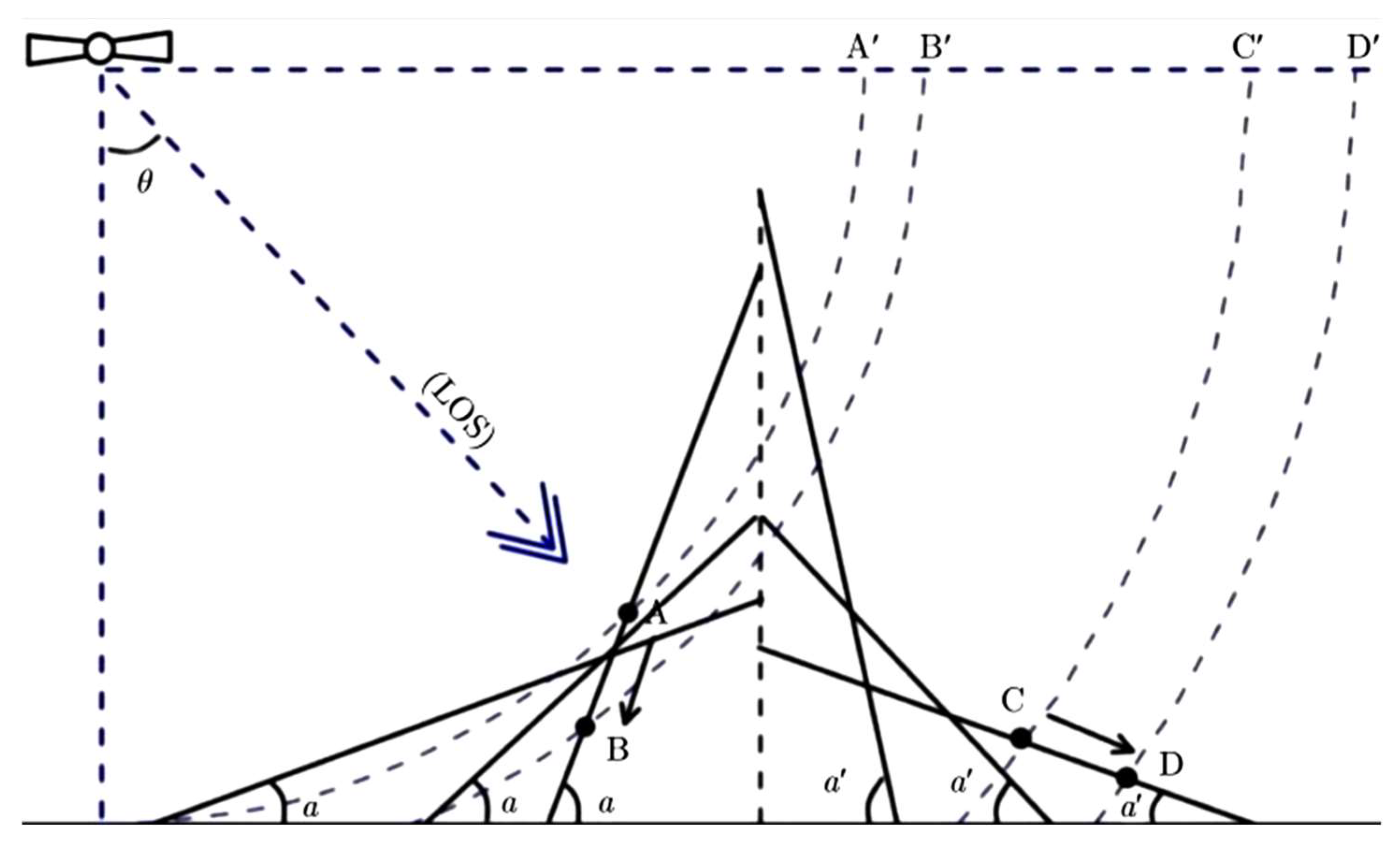
As the SAR satellite sensor produces side-view images, layover, foreshortening, and shadows become more likely to occur when the ground surface has large fluctuations [55]. Layover refers to the echo signals of the top and the bottom of the mountain being reversed; foreshortening refers to the phenomenon in which the backscattered signals from a slope are recorded as one single point, resulting in the aliasing of observation values; and shadows refer to the situation in which there are no observations due to the inability of the radar sensor to monitor the steep back slope [56,57]. Assuming that the incident angle of the satellite sensor is and that is the surface slope, the geometric distortion of the deformation observations corresponding to different incident angles and slopes is shown in Figure 4 and Table 3. It can be seen that when the local surface slope and the satellite incident angle are in a certain geometric relationship, the satellite will not detect the surface deformation. This error will result in missing detection of the landslide, so this situation is an important indicator in data evaluation. In this paper, we classify the fully monitored and foreshortened area as the visible area and layover and shadow area as the invisible area.
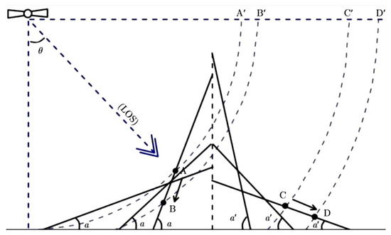
Figure 4.
Schematic diagram of the geometric relationship between satellite incidence angle and observations of slope deformation.
Table 3.
Categories of geometric relationship between satellite incidence angle and observations of slope deformation.
3.4. Coherence of Differential Interferogram Analysis
For a series of radar echoes, if there is similarity between their phase and amplitude, in the radar interference image, this similarity is manifested as interference fringes. Coherence is an index by which to measure the similarity between radar echoes, and the coherence coefficient is a measure of coherence. The coherence between two radar echo signals is γ and can be defined as follows [58]:
Based on this definition, the coherence of each pixel in the interferogram can be calculated. Coherence can usually be used as a measure of the effect of short-wavelength band errors on measurement accuracy; the higher the coherence, the smaller the standard deviation of the interferometric phase and the lower the dispersion of the interferometric phase for the same number of views. When the coherence is lower and the standard deviation of the interferometric phase is larger, the uncertainty of the interferometric phase is greater. Therefore, coherence is an important metric for InSAR data, and higher coherence often means more reliable phase information. During repeated orbit observations, interferometric phase decoherence can be caused by changes in the antenna phase center during satellite flights and changes in the dielectric coefficient of surface objects [59]. Considering the coherence performance of the data, the multi-look factors of 10:2 and 4:3 are used to reduce the decoherence noise of Sentinel−1A and ALOS/PALSAR−2, respectively. In this paper, the average coherence of all interference pairs of two kinds of data is used to evaluate their accuracy.
3.5. Phase Closure Loop Residual
The interferometric phase will introduce new phase errors in the process of difference, unwrapping, etc., resulting in a non-zero phase closure of interferogram triplets. These phase un-closed areas usually appear in the jump of the unwrapping phase [60]. These residuals constitute an important index by which to judge the quality of unwrapped interferometric phases [61]. Assuming that the original phases of three SAR images are , , and , the differential phases of their mutual interference are , , and , and the corresponding unwrapped phases are , , and . Then, the phase closure loop residual can be expressed as [62]:
Due to the influence of residuals such as DEM error, orbit error, and atmospheric error in data processing, there will be phase triangle closed residuals [62]. Therefore, these residuals are an important index by which to judge the quality of the unwrapped image. The RMSE (root mean square error) of the residual error of the unwrapped phase closed loop can reflect how much phase unwrapped error is included in the closed loop [51] so that the quality of the relevant interferogram can be deduced.
4. Results
4.1. Comparison of Annual Deformation Rate
During data processing, it was found that the image quality of the Sentinel−1A data from 28 September 2021, 10 October 2021, and 7 June 2022, was very unsatisfactory. In order to ensure the quality of overall performance, these three images were removed, and the remaining 34 interference pairs were used for subsequent processing. Thus, the deformation data from 22 October 2021, to 2 May 2022 were obtained from Sentinel−1A. After ALOS/PALSAR−2 was optimized, the remaining 25 interference pairs are subjected to subsequent processing. One of these images, the image from 4 June 2022, has a large difference from the phase center of the others and was thus eliminated. The final deformation data were obtained from 25 September 2021 to 7 May 2022. The monitoring accuracies of ALOS/PALSAR−2 and Sentinel−1A are 26.8 m and 9.65 m, respectively.
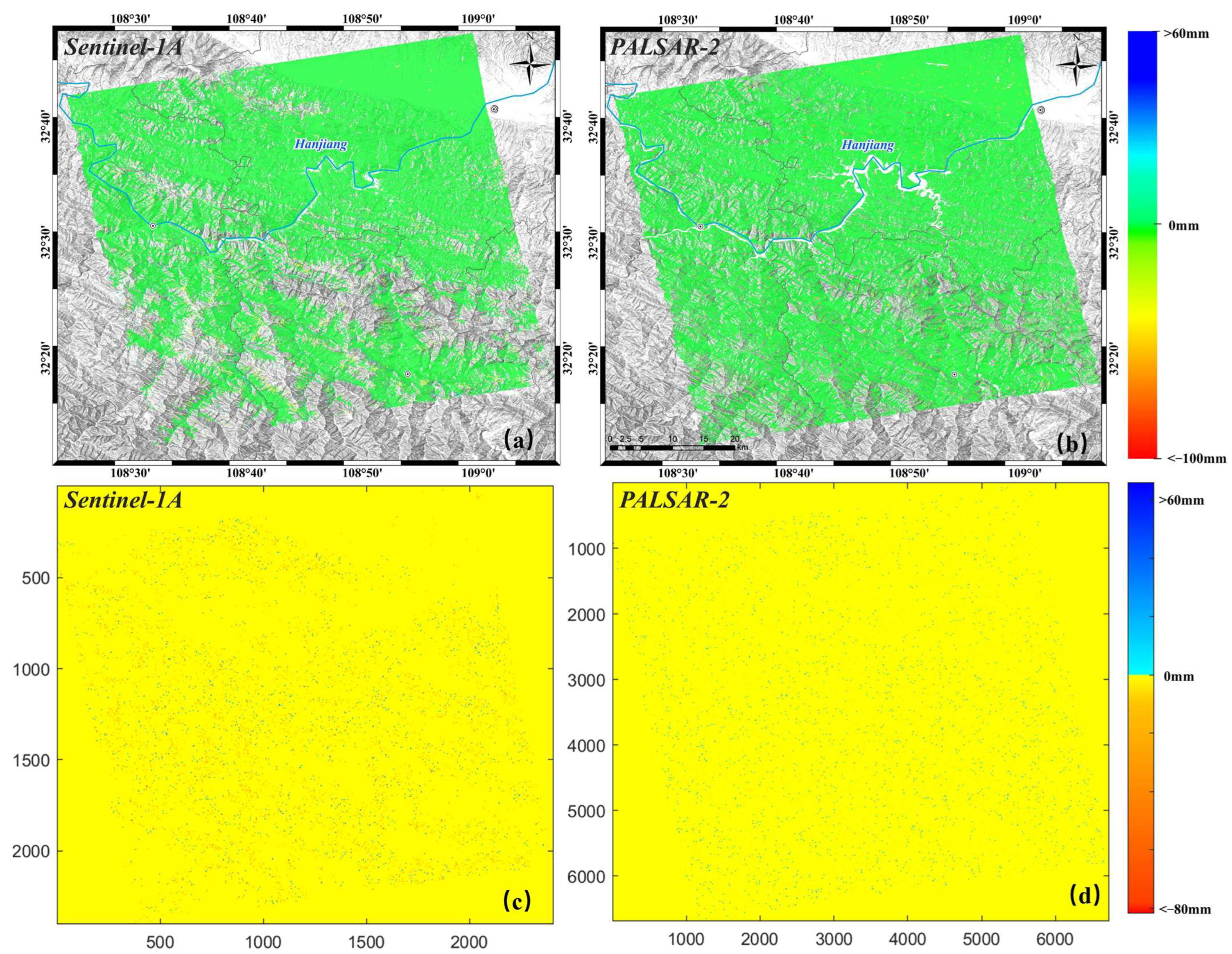
When a region is deformed, most of the deformation-rate pixels should be unstable, with obvious clustering properties [53,63]. These are considered to be real deformation regions, and the error is usually expressed as discrete deformation points. Figure 5a,b show the original deformation-rate results obtained by IPTA−SBAS. Although the atmospheric error, DEM error, and orbital error were removed during data processing, there are still residual and newly introduced error phases. The final result contains some discrete error points, which usually greatly affect the speed and accuracy of subsequent landslide interpretation [63]. The number of discrete error points in the deformation-rate results is also an important indicator of the monitoring quality of SAR data. This experiment uses hotspot-analysis technology to identify obvious cold spots, hotspots, and discrete unstable points in the annual average rate results. The discrete error of Sentinel−1A accounts for 5% of the total error, and the error point is located in the high-vegetation-coverage area. Reliable detection results from built-up areas were validated with almost no discrete error points (Figure 5c). However, most of the slopes in this area are less than 10° and are unlikely to experience landslides. The error ratio of ALOS/PALSAR−2 is 3%; its discrete error points are relatively few and evenly distributed, and the error points are not strongly correlated with terrain changes (Figure 5d). Therefore, the reliability of ALOS/PALSAR−2 is still higher than that of Sentinel−1A in terms of the overall deformation rate.
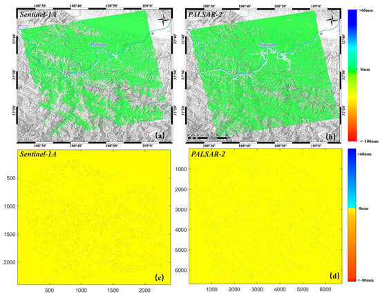
Figure 5.
Original annual line-of-sight (LOS) deformation-rate results. (a,b) represent the annual LOS deformation rates obtained from Sentinel−1A and ALOS/PALSAR−2 data, respectively. A positive value (blue) indicates that the deformation direction detected by the satellite is close to the satellite flight direction, while a negative value (red) indicates that the detected direction of deformation is away from the satellite; (c,d) are the discrete error points in the Sentinel−1A and ALOS/PALSAR−2 velocity diagrams, respectively.
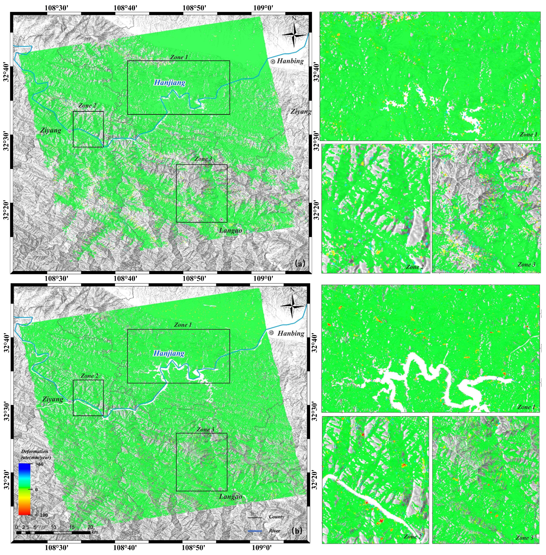
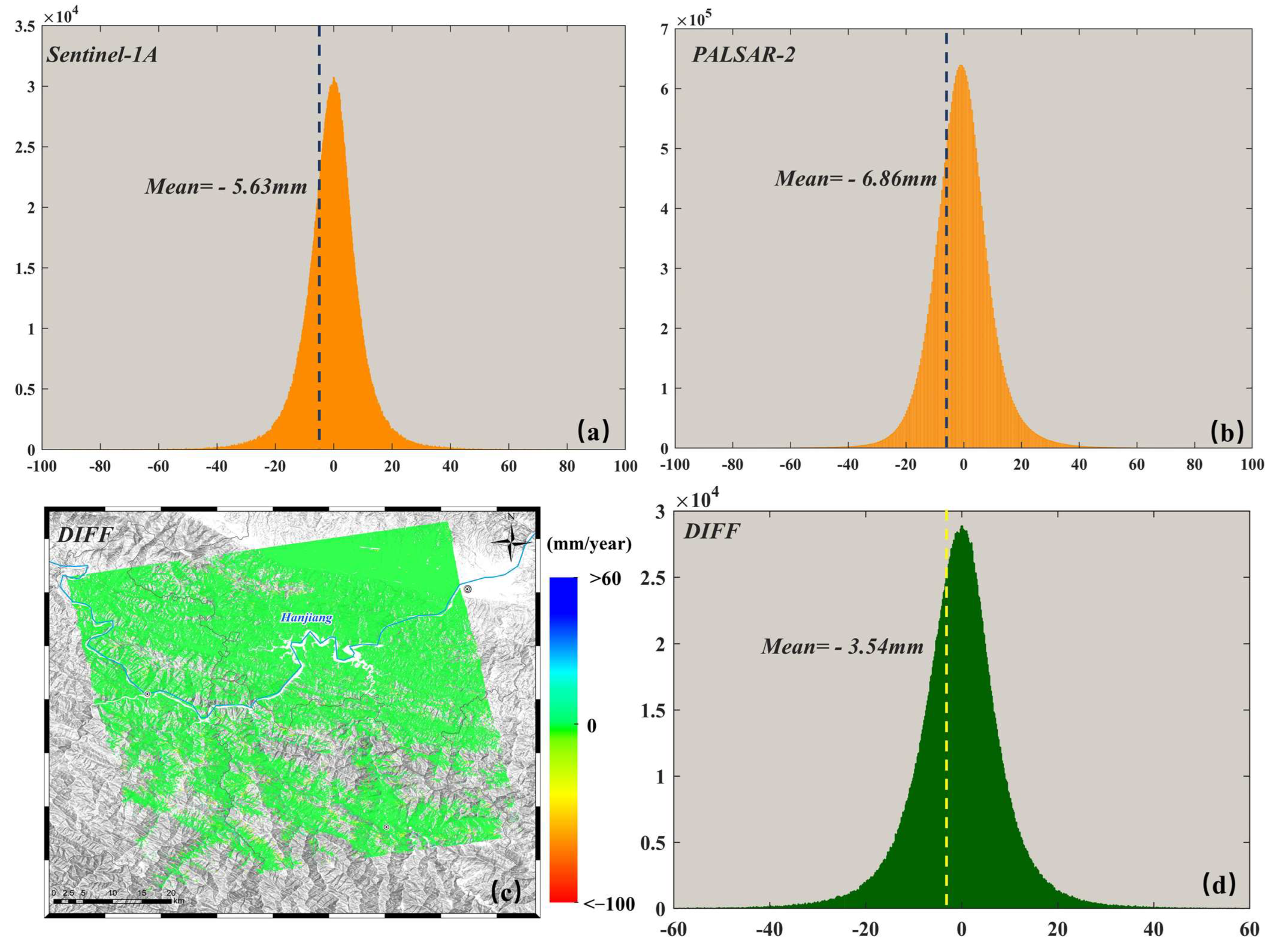
After discrete error points are removed, the final average annual deformation rate is obtained. As shown in Figure 6a,b, the effective monitoring areas of ALOS/PALSAR−2 and Sentinel−1A are 88.4% and 72.58%, respectively. The superior penetration of ALOS/PALSAR−2 makes it theoretically better suited to monitoring potential geohazards. The average annual deformation rates of both data types are close to a normal distribution, and the mean values of Sentinel−1A and ALOS/PALSAR−2 are −5.63 mm/year and −6.26 mm/year, respectively, which indicates that the study area is relatively stable. The difference between the annual average deformation rates of the two is calculated. It is found that points with large differences are mostly distributed in areas with relatively lush vegetation (Figure 7c), and the overall distribution still follows a normal distribution, with an average value of −3.54 mm (Figure 7d). Most of the differences are within ±30 mm, and the data consistency is relatively poor.
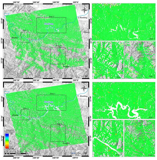
Figure 6.
Diagram of annual LOS deformation rate. (a,b) show results from Sentinel−1A and ALOS/PALSAR−2, respectively. The right side contains the enlarged diagrams of the corresponding zones (Zone 1, Zone and Zone 3).
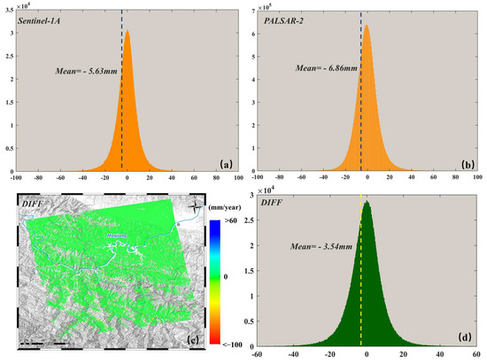
Figure 7.
Diagram of deformation-rate statistics. (a,b) represent the deformation-rate statistics of Sentinel−1A and ALOS/PALSAR−2 data in the LOS direction, respectively; (c) represents the deformation-rate difference between Sentinel−1A and ALOS/PALSAR−2, and (d) is the corresponding statistical graph.
In order to analyze the difference in deformation rate between the Sentinel−1A and ALOS/PALSAR−2 data in more detail, three areas where the deformation is concentrated (Zone 1, Zone 2, and Zone 3 in Figure 6) are investigated more closely. In Zone 1, which has low vegetation coverage, although Sentinel−1A is able to recognize most of the deformed areas detected by ALOS/PALSAR−2, it found deformation-rate values and landslide-activity ranges that were generally smaller than those detected by the latter. In this case, the rate of missed judgments in subsequent interpretations would increase. In Zone 2, which has medium vegetation coverage, Sentinel−1A missed six large deformation areas that ALOS/PALSAR−2 did not. In Zone 3, which has extremely high vegetation coverage, not only are the deformation rates of the two data sources quite different, but the effective monitoring area of Sentinel−1A is also greatly reduced. Sentinel−1A and ALOS/PALSAR−2 missed eleven and five concentrated deformations, respectively. In general, ALOS/PALSAR−2 has vast advantages over Sentinel−1A in detection of the deformation rate.
4.2. Comparison of Landslide Detection Results
In this paper, the deformation-rate results obtained by InSAR technology are superimposed on the three-dimensional Google images, and the three-dimensional optical image is used to assess the disaster-producing conditions and deformation signs of the deformed area. Usually, a landslide will result in local changes in optics, and there will be ground fissures, small collapses, and bare areas. The vegetation index is significantly reduced. If the optical signs conform to the characteristics of the landslide and there are certain indicators of risk, the area is preliminarily judged as a potential landslide, more than 80% of the which are verified in the field. Finally, a total of 88 landslides were identified in the study area (Figure 8), and 66 of them were investigated in the field; others that have not been verified also show obvious deformation traces in the optical time-series images. It is clear IPTA−SBAS is able to detect landslides in the Qinling–Daba Mountains. Through analysis, we found that landslides in this area mostly occurred on both sides of the river. First, the river is a densely populated area, which indicates the influence of engineering [64]; second, long-term erosion by the river will also reduce the stability of the slope [65,66].
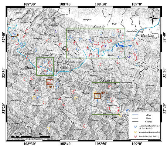
Figure 8.
Inventory map of detected landslides. HP 1, HP 2 and HP 3 are Hujiayuan landslide, Lianfengcun landslide and Sanxingwan landslide, respectively; In this figure, Zone 1, Zone 2 and Zone 3 correspond to those in Figure 6.
Landslides in the Qinling-Daba Mountains are mainly shallow, small and medium-sized, with clear seasonality [33]. The superior penetration and high spatial resolution of ALOS/PALSAR−2 enabled that system to identify 80 landslides in this area (Figure 8). Accounting for 90.9% of the total number of detected landslides, it shows excellent detection performance. However, Sentinel−1A detected only 38 landslides in this area, accounting for 43.2% of the total number. Furthermore, 50 landslides were detected only by ALOS/PALSAR−2; most of these are small, seasonal, and located near rivers. Additionally, eight landslides were detected only by Sentinel−1A, most of which are distributed in the alpine and canyon areas with dense vegetation and steep slopes. Generally, ALOS/PALSAR−2 has absolute detection advantages in areas of dense vegetation [67,68], but it still missed eight landslides in our experiment.
4.3. Comparison and Verification of Typical Landslides
In order to illustrate the accuracy of the recognition results and compare the results of the two systems, three landslides were selected: one that was detected by both data sources (Hujiayuan landslide), one that was detected only by ALOS/PALSAR−2 (Lianfengcun landslide), and one that was detected only by Sentinel−1A (Sanxingwan landslide). The locations of the landslides are marked in Figure 8. The deformation along the LOS direction was changed to the vertical direction for better comparison of monitoring results.
4.3.1. Hujiayuan Landslide
The Hujiayuan landslide is located in Miaoxi Village, Huangu Town, Ziyang County; the slope is 26°, and the elevation is 112 m. The average annual precipitation is 1066.2 mm, mostly concentrated from mid- and late June to early October. This landslide is a thrust-type landslide, which can be detected by both data sources.
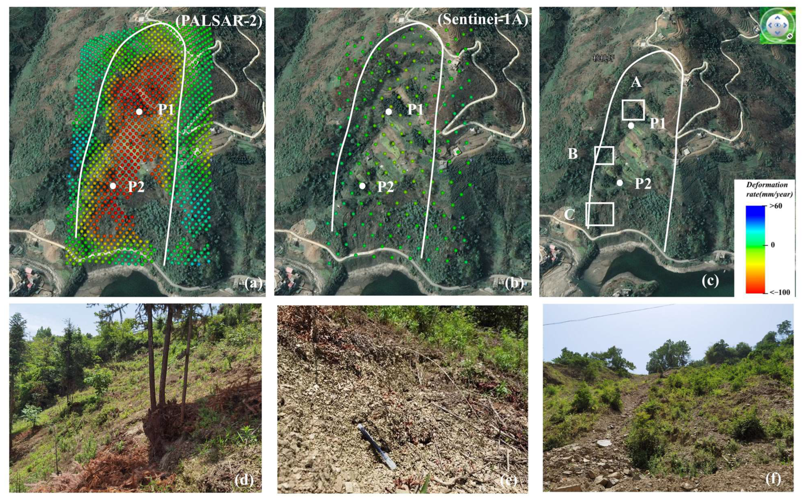
A field survey shows that the landslide is covered with a large number of scattered gravel soil blocks. Point P1 is the back of the landslide (Figure 9d), where the soil is exposed, and obvious traces of decline can be observed. Small collapses can be seen everywhere on the slope body (Figure 9e), and there are many cracks in the side walls of the houses and the cement road (Figure 9f), which is consistent with the results from deformation monitoring. The deformation rates found from the two data types across the time coverage are different, as shown in Figure 9a,b: the annual deformation-rate range found by ALOS/PALSAR−2 is −124 mm~19 mm/year, while that found by Sentinel−1A is −94.5 mm~13 mm/year. The deformation ranges detected by Sentinel−1A and ALOS/PALSAR−2 are nearly the same, but the latter can clearly detect more deformation details due to its superior resolution.
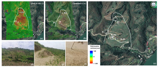
Figure 9.
Hujiayuan landslide. (a,b) show annual deformation-rate results from ALOS/PALSAR−2 and Sentinel−1A, respectively. (c) is the optical image on Google Earth; (d–f) are the field-survey pictures showing the areas in white boxes A, B and C in (c), respectively. The P1 and P2 points marked on the figure are the points for time series deformation analysis in chapter 5.4.1.
4.3.2. Lianfeng Landslide
The Lianfeng landslide is located in Lianfeng Village, Donghe Town, Ziyang County; the slope is about 42°, and the elevation is 198 m. A field survey found that a 3~5 m-high scarp was formed on the posterior border (Figure 10d), and staggered scarps and cracks were seen on the flank (Figure 10e). There are many tension cracks on the slope, and the collapse of the toe is obvious (Figure 10f).

Figure 10.
Lianfeng landslide. (a,b) show annual deformation-rate results from ALOS/PALSAR−2 and Sentinel−1A, respectively. (c) is the optical image on Google Earth; (d–f) are the field-survey pictures showing the areas in white boxes A, B and C in (c), respectively. The P1 and P2 points marked on the figure are the points for time series deformation analysis in chapter 5.4.2.
The field-survey results verified the validity of monitoring landslides using ALOS/PALSAR−2. The deformation of this landslide is obvious on ALOS/PALSAR−2, with an average annual deformation rate of 15 mm~79.8 mm/year; however, the results of Sentinel−1A show that this area is relatively stable, with an annual deformation rate of −13 mm~10 mm/year. The vegetation coverage here is thick, which is why even though the deformation is obvious, the Sentinel−1A data still failed to detect it.
4.3.3. Sanxingwan Landslide
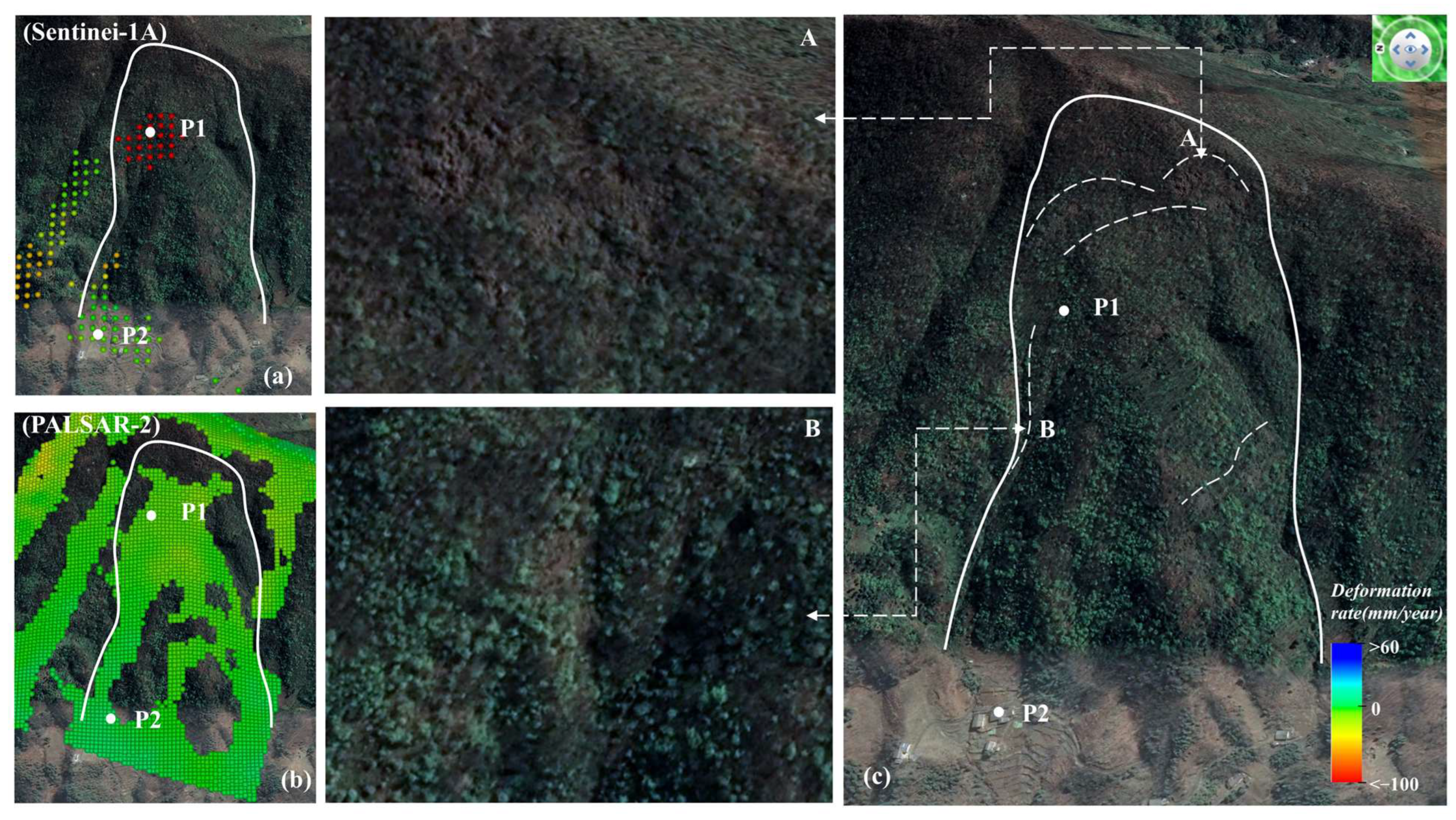
The Sanxingwan landslide is located in Sanxingwan Village, Minzhu Town, Langao County, and the elevation is 296 m. It is a large landslide, and the vegetation coverage is moderate, with small, sparse shrubs growing. This landslide was detected only by Sentinel−1A. The landslide is difficult to reach and there are no field verification data; however, validation can still be carried out via optical-image interpretation. Four large tensive cracks can be clearly seen in the optical image. Additionally, the flank of the slope body is relatively deep and the crown on the slope body is obviously observed (Figure 11c). Although Sentinel−1A is mostly decoherent in this area, a concentrated deformation area was detected on the left back of the slope (Figure 11a). The coherence of ALOS/PALSAR−2 is relatively good in this area, but the monitoring results show that there is no obvious deformation (Figure 11b), which indicates a missing detection in this area.
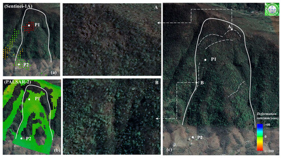
Figure 11.
Sanxingwan landslide. (a,b) show annual deformation rate results of ALOS/PALSAR−2 and Sentinel−1A, respectively. (c) is the optical image on Google Earth. The P1 and P2 points marked on the figure are the points for time series deformation analysis in chapter 5.4.3.
4.4. Overall Adaptability Analysis
In order to more clearly compare the detection capabilities of the two data-gathering systems, we summarized their indicators and detection results, as shown in Table 4 and Figure 12. In general, although Sentinel−1A has a short revisit cycle and can obtain more data, the proportions of data and interference pairs available in data processing are 5.79% and 13.94% lower, respectively, than the proportions available from PALSAR−2, (Table 4). The discrete error point in the deformation rate is 2% higher than that of PALSAR−2, and the effective monitoring area of the deformation rate is 15.82% lower. In terms of accuracy in detecting the deformation rate, PALSAR−2 is 2.78 times more accurate than Sentinel−1A. In summary, Sentinel−1A is far less well-suited than PALSAR−2 to detecting landslides in complex and dangerous areas. Therefore, its total detection rate is 47.7% lower than that of PALSAR−2. Because of the low detection rate, we combined the characteristics of Qinling–Daba Mountains landslides and the characteristics of two data sources to analyze our results.
Table 4.
Indicators of Sentinel−1A and PALSAR−2 data.
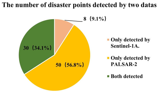
Figure 12.
The number of disaster points detected by two data-collection systems.
5. Discussion
In order to further explore the difference between the two data types in detecting landslides, the following section presents a detailed analysis of the four aspects of visibility, coherence, unwrapped phase closed-loop residuals, and deformation time-series data for typical landslides.
5.1. Data Visibility Analysis
According to the geometric relationships and categories mentioned in Section 3.3, we calculated the visual area of the image and combined it with radar incident angle and DEM data. The incident angles of the ascending Sentinel−1A and the ALOS/PALSAR−2 ascending satellite used in this paper are 37.76° and 36.18°, respectively, so the difference is small. The proportion of visible area of Sentinel−1A is 88.50%, and that of ALOS/PALSAR−2 is 87.55% (Figure 13). The visibility of Sentinel−1A is slightly higher than that of ALOS/PALSAR−2, but the proportions of visible and geometrically distorted areas are almost the same. Therefore, the difference in the detection results is not likely to have been caused by geometric distortion.
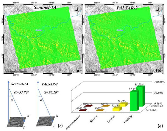
Figure 13.
Schematic diagram of visible and geometric distortion areas; (a,b) are schematic diagrams of the visual and geometric distortion areas of Sentinel−1A and ALOS/PALSAR−2, respectively; (c) shows the incident angle of Sentinel−1A and ALOS/PALSAR−2; (d) is a statistical diagram of Sentinel−1A and ALOS/PALSAR−2 visibility, layover, shadow, and layover-shadow areas. Here, the ribbon settings of (a,b) are consistent with (d).
5.2. Analysis and of Coherence of Differential Interferogram
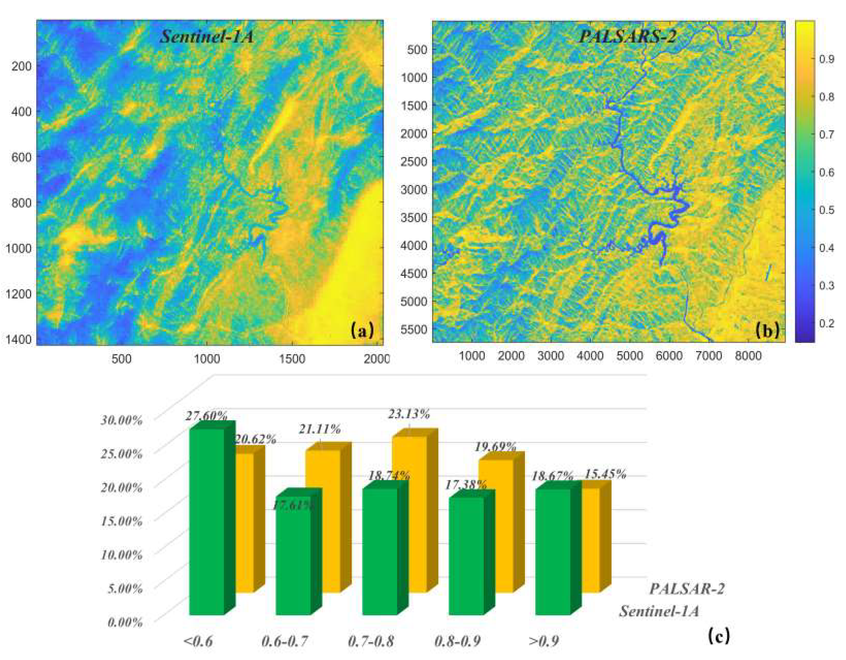
As defined and described in Section 3.4, the average coherence coefficient of the high-quality interferogram that yields the annual average deformation rate and time series is calculated, and the results are shown in Figure 14. Due to Sentinel−1A’s advantage in time sampling of, the proportion of values with coherence greater than 0.9 is 3.22% higher than that of ALOS/PALSAR−2. However, the overall coherence is lower than that of ALOS/PALSAR−2, and the proportion of regions with coherence greater than 0.6 is 6.98% lower than that of ALOS/PALSAR−2. In some areas with more artificial construction and less vegetation, Sentinel−1A shows extremely strong coherence, and ALOS/PALSAR−2 still has some sporadic low-coherence areas inside the high-coherence areas. The coherence of Sentinel−1A is strongly correlated with the type of surface scatterers, while the variation in the coherence of ALOS/PALSAR−2 across different surface scatterers is relatively small. The decoherence of ALOS/PALSAR−2 is mainly caused by its long temporal baseline. In conclusion, ALOS/PALSAR−2 has a coherence advantage over Sentinel−1A in areas with dense vegetation. This difference in coherence leads to a lower effective detection area in the Sentinel−1A deformation-rate results, so the final number of detected landslides will be lower than the number detected by PALSAR−2 (especially in areas with high vegetation coverage).
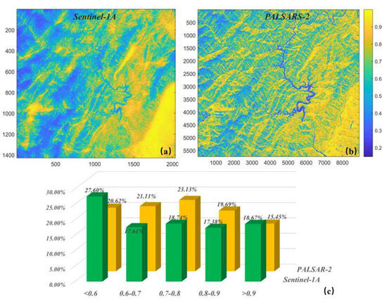
Figure 14.
Evaluation of coherence coefficients. (a,b) represent the average coherence coefficients of Sentinel−1A and PALSAR−2, respectively. The values of coherence coefficients from small to large (0 to 1) are represented by shading from blue to yellow, respectively. (c) is the statistics of the coherence coefficient of two data sources.
5.3. Analysis of Unwrapped Phase Closed-Loop Residuals
Based on research and experience [69], a closed loop is considered a problem loop when the RMSE (as explained in Section 3.5) is greater than 1.5 rad. If all the closed loops related to a certain interferogram have problems, it is considered that the interferogram may contain more phase unwrapping errors [62]. As shown in Table 5, in this experiment, 55 interference pairs generated by Sentinel−1A data constituted a total of 64 closed loops, of which one scene datum (20220607) could not form a closed loop with the other data due to the large space-time baseline. Among the closed loops, there are 20 closed loops whose RMSEs are less than 1.5 rad and 44 closed loops whose RMSEs are greater than 1.5 rad, and the problematic loops account for 68.7% of the total. Thus, 21 problematic interference pairs were identified and eliminated in subsequent processing. ALOS/PALSAR−2 formed 52 closed loops, 17 of which had an RMSE greater than 1.5 rad, accounting for 32.7% of the total, and eight interference pairs were included in the problematic closed loop. Sentinel−1A has a 36% higher rate of problematic loops compared with ALOS/PALSAR−2.
Table 5.
Proportion of problem loops among all unwrapped phase closed loops.
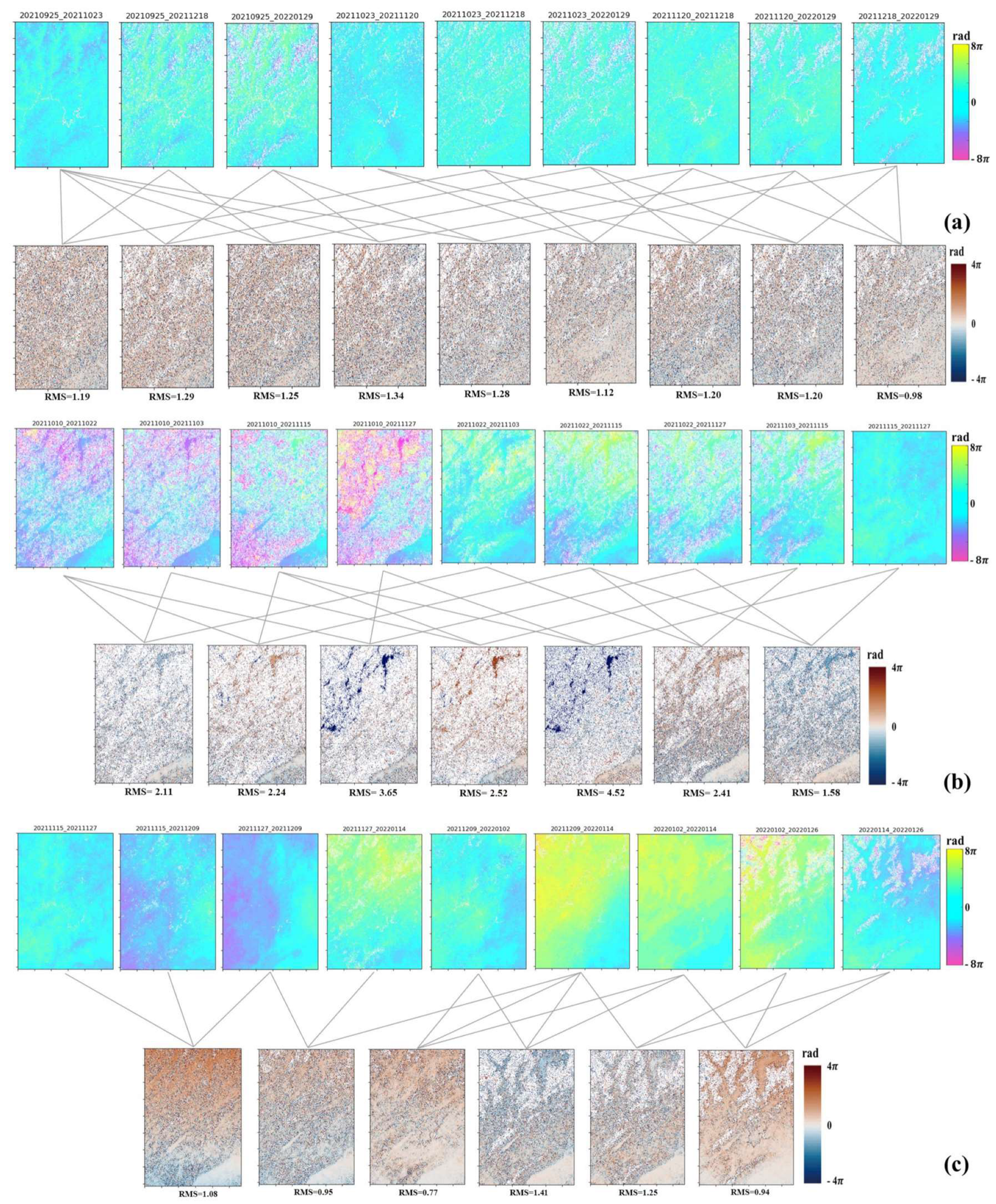
For further analysis, samples of unwrapped images and closed-loop residuals of the two data sources were selected, as shown in Figure 15. Even if the temporal baseline is short, the image quality of Sentinel−1A in mountainous areas will still be extremely poor and the RMSE of all closed loops will exceed the limit (Figure 15b). It is clear that large closed-loop residuals are mostly concentrated in areas with high vegetation. However, when the vegetation coverage is low and the surface is more bare in winter, its overall RMSE is small and the interference quality is better than that of ALOS/PALSAR−2 images taken at the same time (Figure 15a,c). In addition, the Sentinel−1A data also showed better interference quality for areas containing more buildings. ALOS/PALSAR−2 data are less affected by vegetation or seasonal changes and can still maintain relatively good interference quality for a long time (Figure 15a).
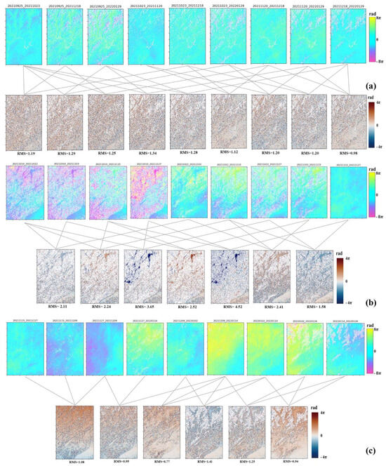
Figure 15.
The unwrapping and closed-loop residuals diagram; (a) the unwrapping images and the closed-loop residuals from ALOS/PALSAR−2 from 25 September 2021 to 29 January 2022; (b) the unwrapping images and the closed-loop residuals from Sentinel−1A from 10 October 2021 to 27 November 2021; (c) the unwrapping images and the closed-loop residuals from Sentinel−1A from 27 November 2021 to 26 January 2022.
From the RMSE of the phase closed loop of the interference pair, even if the same time coverage is selected, Sentinel−1A is prone to obtaining continuous low-quality interference pairs in summer and thus should be completely eliminated in the subsequent processing, resulting in the direct loss of data in some continuous time series. This problem can lead to the phenomenon in which the deformed regions detected by ALOS/PALSAR−2 are stable in the Sentinel−1A results and the overall agreement between the two in terms of the deformation rate is also poor. In addition, with the increase in vegetation coverage, the periodic and seasonal characteristics of landslides in the Qinling–Daba Mountain Area are becoming increasingly prominent [2,3]. The lack of summer data will directly lead to failure to detect many sudden landslides. Un this experiment, the low-vegetation area with excellent Sentinel−1A performance is in the city, where it is uncommon for landslides to occur. In short, Sentinel−1A has poor performance because of its poor detection ability in high-vegetation areas and because of the characteristics of seasonal landslides in the Qinling–Daba Mountains.
5.4. Analysis of Typical Landslides
In order to further discuss why the detection results of the first three typical landslide points are inconsistent or why some landslides were not even detected, the deformation time-series data results are extracted for each of them separately.
5.4.1. Hujiayuan Landslide
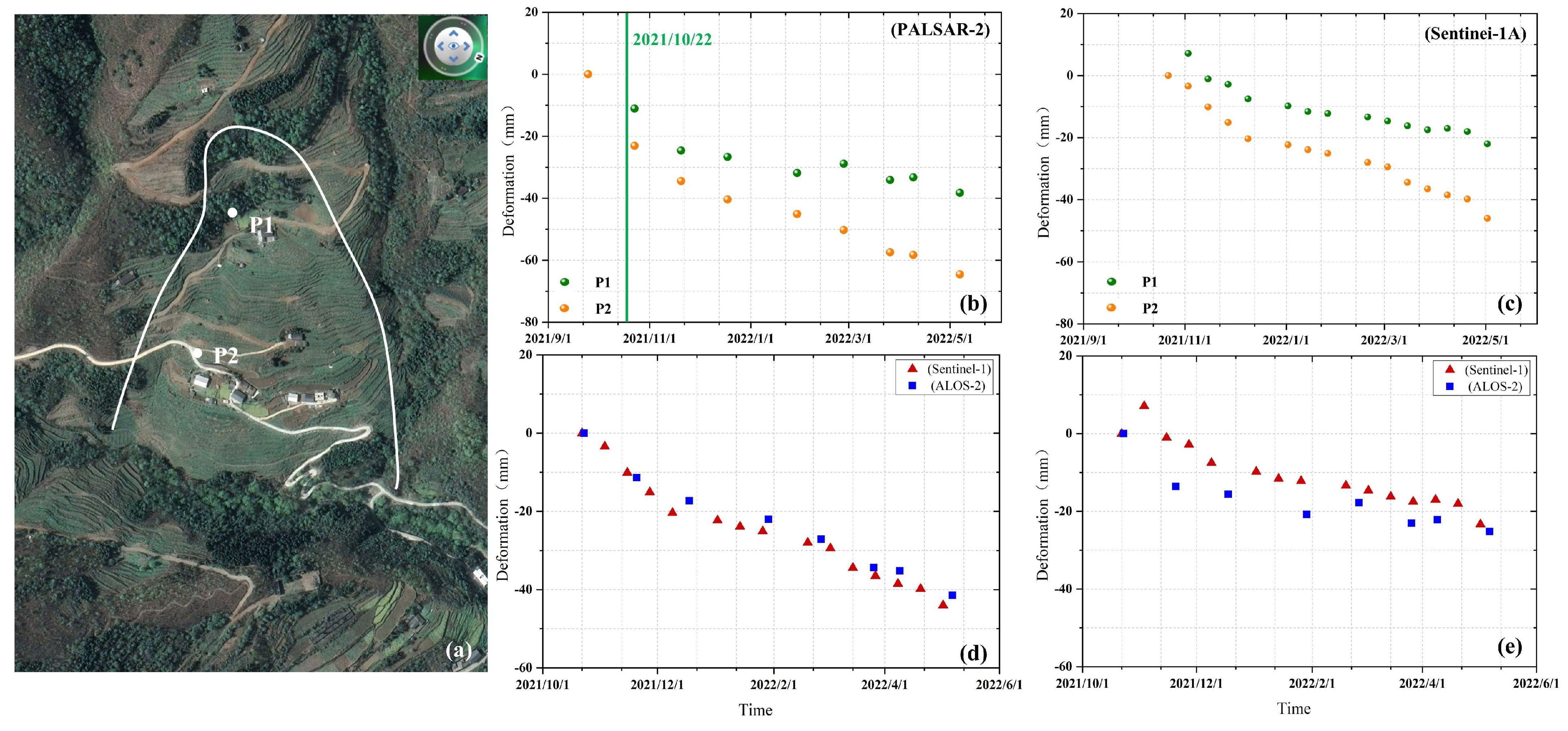
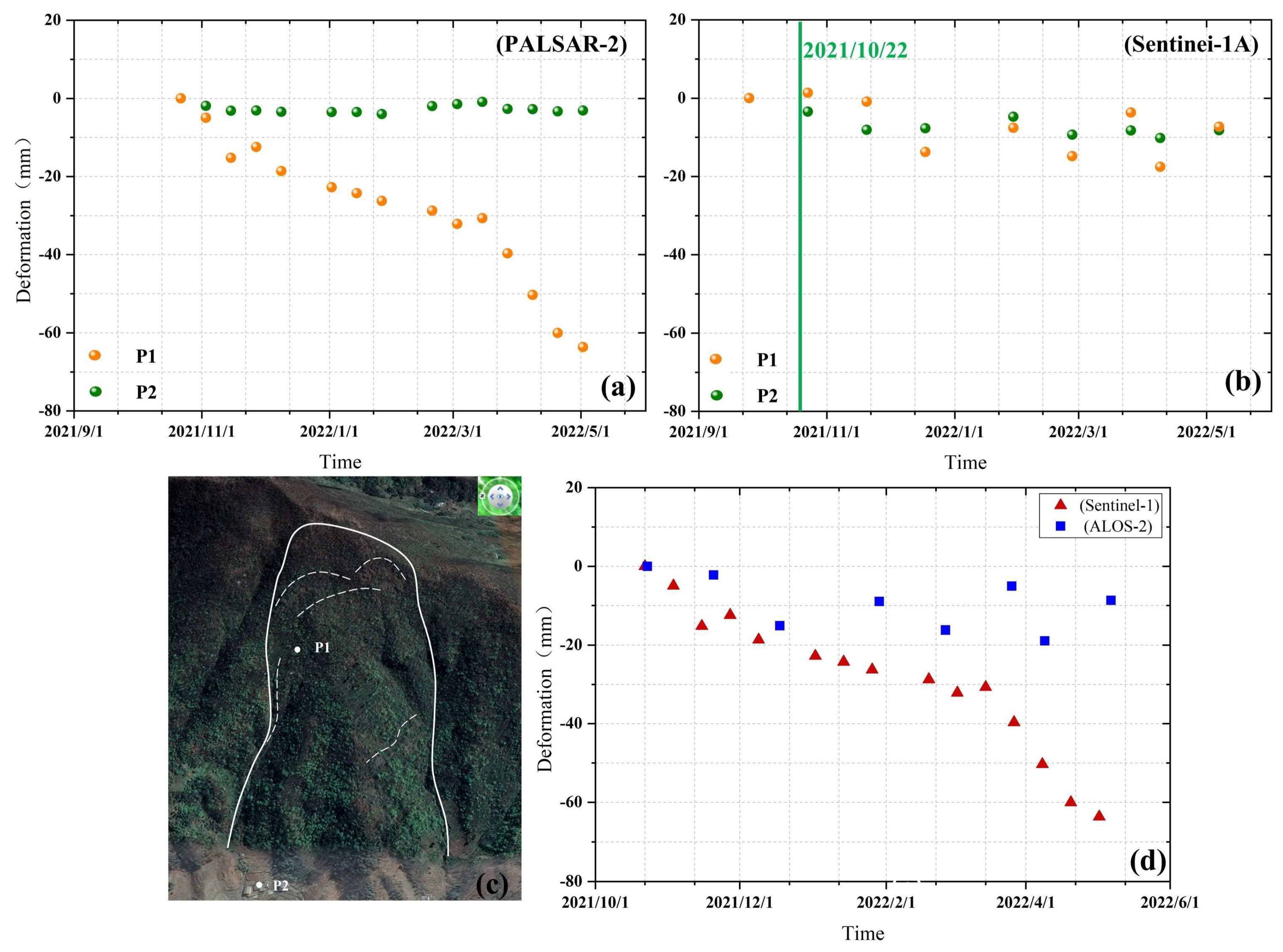
Two time series on the trailing edge and leading edge of the Hujiayuanzi slope are extracted and shown as points P1 and P2 in Figure 16a. The cumulative deformation of point P1 detected by ALOS/PALSAR−2 is −64.54 mm, and that of Sentinel−1A is −44.01 mm, with a difference of 20.53 mm. Meanwhile, the deformation of point P2 detected by ALOS/PALSAR−2 is −36.25 mm, and that of Sentinel−1A is −23.35 mm, with a difference of 12.9 mm. In order to make a more intuitive comparison, the consistency analysis of the time series trend was performed after the time difference was removed from the cumulative deformation of the two data. Figure 16d shows the cumulative time-series results after the time difference was removed at point P1. High consistency can be observed in the monitoring results, and the trend in the deformation of point P1 is close to linear. Figure 16e shows the time-series results of point P2 after the time difference was removed. High consistency is also observed here. The trend in the deformation of the landslide is relatively steep before January 2021 but relatively slower after that. It is clear that in areas with relatively low vegetation coverage, the deformation trends detected by the two data sources are relatively consistent. The time-series results verified that the deformation rate detected by Sentinel−1A is generally lower than that detected by ALOS/PALSAR−2 because of the unavailability of summer monitoring data.
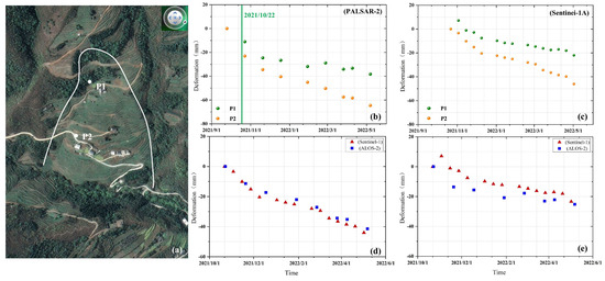
Figure 16.
InSAR time-series results for the Hujiayuan landslide; (a) is the optical image of the landslide, and the positions of PI and P2 points are marked on the image; (b,c) are the time-series results from ALOS/PALSAR−2 and Sentinel−1A at P1 and P2, respectively; (d,e) are comparisons of time series between P1 and P2 after the time difference was removed.
5.4.2. Lianfeng Landslide
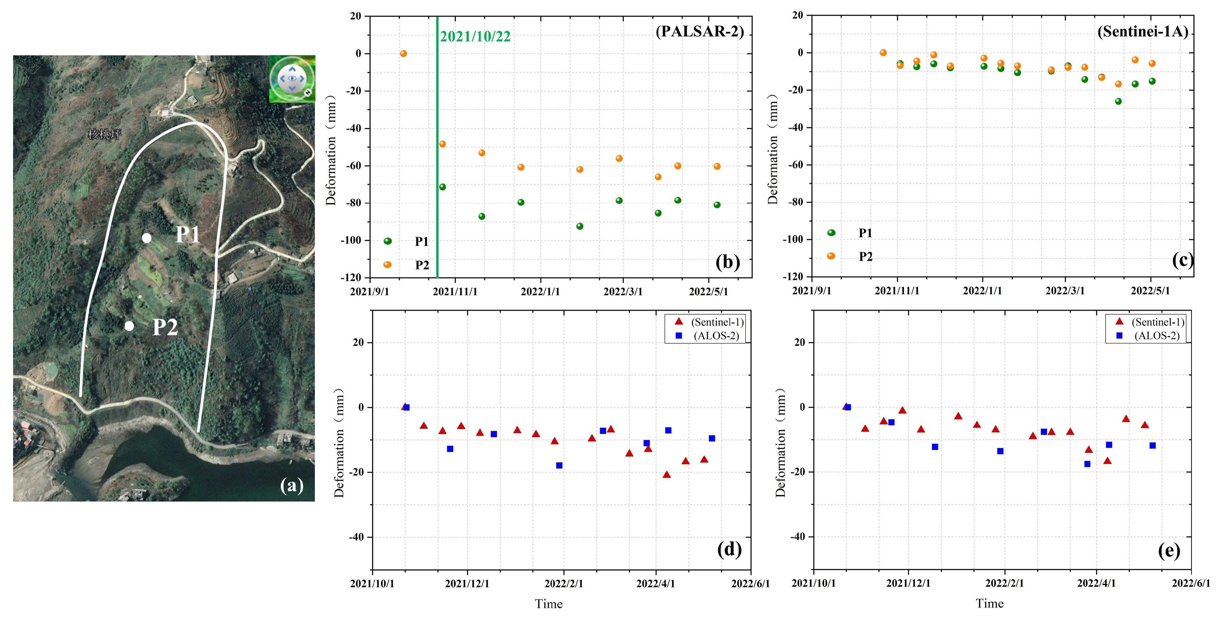
After the time series of the upper part (P1 point) and lower part (P2 point) of the Lianfeng landslide was extracted (Figure 17a), the ALOS/PALSAR−2 time-series results of P1 and P2 showed severe deformation during the period 26 September~22 October 2021. During this period, the cumulative deformation of P1 reached −71.39 mm, and the sequential deformation has been fluctuating since then. The cumulative amount of deformation reached −80.93 mm on 2 May 2022 (Figure 17). P2 shows similar trends to P1. After the time difference between the time-series results of the two data sources was removed, the two were in good agreement, indicating that the deformation of the landslide was concentrated before 22 October and Sentinel−1A missed monitoring due to the low coherence of summer data. The summer rainfall in the Qinling-Daba Mountains is concentrated, and excessive rainfall will directly lead to large displacement or failure of the slope, causing sudden seasonal landslides [70]. The time-series results further confirm the landslide characteristics of the Qinling-Daba Mountains. The reason for non-detection of landslides by Sentinel−1A is also clarified.

Figure 17.
InSAR time-series results of Lianfeng landslide, (a) is the optical image of the landslide, and the positions of PI and P2 points are marked on the image; (b,c) are the time-series results of ALOS/PALSAR−2 and Sentinel−1A at P1 and P2, respectively; (d,e) are comparison of time series between P1 and P2 after removing the time difference.
5.4.3. Sanxingwan Landslide
The time series of P1 on the back and P2 on the toe of the Sanxingwan landslide (Figure 18c) were extracted for further analysis. As shown in Figure 18a,b, P2 on the leading edge remained stable during monitoring. At P1 on the back of the slope, the Sentinel−1A data showed continuous deformation (Figure 18a), while the deformation time-series data of ALOS/PALSAR−2 oscillated back and forth without any obvious pattern (Figure 18b). Figure 18d was obtained by removing the time difference between the two time series at P1. It can be seen that the cumulative deformation of the two has some consistency before December 18, 2021, but after that time, ALOS/PALSAR−2 shows irregular oscillations, indicating that the results are distorted by errors. The first reason is that radar satellites are more susceptible to atmospheric delay in mountainous areas with steep terrains [71,72] and that L−band sensors will be affected by the ionosphere six times more than X-band ones [70] (atmospheric error is divided into tropospheric error and ionospheric error). Secondly, the spatio-temporal filtering method adopted in this paper requires a large number of original SAR images (usually no fewer than 15 scenes) to be superimposed and calculated when the atmospheric delay phase is separated and removed. The effective data volume of ALOS/PALSAR−2 is only nine scenes, so the ability to remove atmospheric errors will be greatly reduced. Thirdly, ALOS/PALSAR−2 data are not as sensitive to small deformations as Sentinel−1A data are. With the combination of these sensors, a few potential landslides are missed, but the system can still carry out more than 90% of the required monitoring.
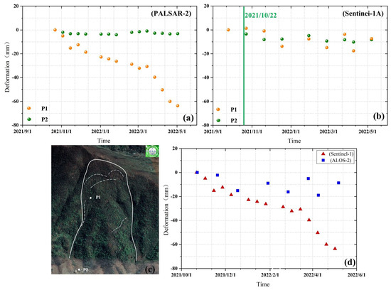
Figure 18.
InSAR time-series results for the Sanxingwan landslide, (a,b) are the time-series results from ALOS/PALSAR−2 and Sentinel−1A at P1 and P2, respectively; (c) is the optical image of the landslide, and the positions of PI and P2 points are marked on the image; (d) is the time series of P1 after the time difference was removed.
5.5. Limitations of the Experiment
Although this experiment included extensive quantitative and qualitative analysis of Sentinel−1A and ALOS/PALSAR−2 data and analyzed their potential for adaptation to in landslide detection in detail, the following deficiencies remain:
- Due to the different revisiting times of the two data sources (three days apart), it is impossible to maintain strict consistency in the date selection of the two data sources, which will lead to a degree of deviation in the final result.
- Many errors will be introduced in data processing, such as registration errors, DEM errors, baseline errors, and unwrapping errors. These errors will ultimately affect the accuracy of the results.
- When selecting the unwrapping reference point, although the selection has been restricted to a certain region as far as was possible, the inconsistent pixel size makes it impossible to maintain the complete unity of the unwrapping reference point. This constraint is also an important factor in the generation of image results.
- This paper uses only IPTA−SBAS technology to compare the adaptability of the two data sources, and it is impossible to determine whether the results are consistent with those obtained using other methods, which will be a focus of future research.
- The research area selected in this paper is very typical of the region, but the coverage is small, and it may not fully represent the complex geographic area. More data will be used for analysis and comparison in the future.
6. Conclusions
In this paper, deformation was extracted using two data sources, Sentinel−1A and ALOS/PALSAR−2, based on the combination of IPTA and SBAS technology. Landslides were further interpreted by identifying deformation and integrating optical and geological factors, and 88 active landslides were observed in the region. Based on the hotspot analysis, there are many discrete error points in the Sentinel−1A rate results (2% more than in the results from ALOS/PALSAR−2), and there are also many missed detections in the concentrated deformation area. The deformation-rate consistency is poor, and the final landslide recognition rate of Sentinel−1A is also 47.7% lower than that of ALOS/PALSAR−2. A comparative analysis of the visibility, coherence, closed-loop residuals, and time series of individual landslides from the two data types shows that the main reason for their differences is that the quality of Sentinel−1A’s summer data is extremely low, resulting in missed detection of many landslides. ALOS/PALSAR−2 is less affected by surface scatterers and time decoherence and is more likely to detect landslides in summer. This advantage makes it highly suitable for landslide detection in the Qinling–Daba Mountains, where seasonality is a significant factor, and this system can meet more than 90% of the monitoring needs.
The time consistency of the two data sources is guaranteed to the greatest extent when the original data are selected, which leads to a smaller amount of Sentinel−1A data being included in the experiment. However, if this factor is not considered in the detection process, Sentinel−1A has the advantages of sufficient free data sources, which prolong its monitoring time. It could thus obtain better results than those seen in this experiment. However, for those areas with sudden deformation in summer and continuous oscillation of deformation trends, serious loss of coherence in dense vegetation and excessive deformation ranges mean that detecting landslides using Sentinel−1A data remains a difficult task. Therefore, when large-scale landslide detection is carried out, the time coverage of Sentinel−1A data should be extended as far as possible, including at least the data from before and after summer (best if these data are available for more than one year). For the key areas with high vegetation coverage and obvious seasonality, it is necessary to use ALOS/PALSAR−2 data for monitoring, and the amount of ALOS/PALSAR−2 data should be greater than 15 scenes to obtain the best effect (so as to better offset the impact of atmospheric errors).
In this paper, a large number of accuracy indicators are used to evaluate the detection capabilities of Sentinel−1A and ALOS/PALSAR−2 in the Qinling–Daba Mountains. These systems are compared in detail for the first time, and the drivers of differences in these systems’ data are also discussed. A more intuitive analysis verifies the feasibility of using two data sources for landslide detection and the necessity of using multi-source data detection in densely vegetation-covered areas. It is believed that this study can provide good suggestions for the selection of data sources for landslide detection in the Qinling–Daba Mountains and similar complex, dangerous mountainous areas with high vegetation coverage and large numbers of shallow landslides. The study also provides important scientific support for the selection of InSAR monitoring accuracy-evaluation methods. Although the experiment was as rigorous as possible, there are still some shortcomings in the data processing, such as inconsistent parameters, the use of a single data-processing method, and the small coverage. For future research, more data-processing methods, such as Stack−InSAR and PS−InSAR technology, should be used to fully verify the applicability of the data. More data sources should also be mined and compared. Of particular interest are the L−band L−SAR data just launched by China, as this system has completed testing and obtained excellent results. Its time resolution is 4 days, and it is believed that it can obtain better time-series monitoring results than ALOS/PALSAR−2.
Author Contributions
Conceptualization, S.Y. and J.Z.; Methodology, S.Y.; Validation, J.Z.; Formal analysis, C.C.; Investigation, S.Y.; Resources, C.C.; Data curation, W.Z.; Writing—original draft, S.Y.; Writing—review & editing, Z.L.; Visualization, Z.L.; Supervision, L.F.; Project administration, W.Z. All authors have read and agreed to the published version of the manuscript.
Funding
This research received no external funding.
Institutional Review Board Statement
Not applicable.
Informed Consent Statement
Not applicable.
Data Availability Statement
The ALOS/PALSAR-2 data used in this study were provided by JAXA, Japan, https://auig2.jaxa.jp/ips/home (accessed on 21 May 2023); The Sentinel-1A images were provided by the European Space Agency (ESA) freely through the Sentinels Scientific Data Hub, https://search.asf.alaska.edu (accessed on 15 July 2023); The one arc-second SRTM DEM was freely downloaded from the website https://e4ftl01.cr.usgs.gov/MEASURES/SRTMGL1.003/2000.02.11/ (accessed on 15 July 2023).
Conflicts of Interest
The authors declare no conflict of interest.
References
- Fei, Q.; Zhao, F.; Dang, Y. Correlation analysis between geological hazards and impact factors in Qinling-Daba Mountains of Southern Shaanxi. South North Water Transf. Water Sci. Technol. 2015, 13, 557–562. [Google Scholar]
- Meng, Q.; Zhang, G. Geologic framework and tectonic evolution of the Qinling Orogen, Central China. Tectonophysics 2000, 323, 183–196. [Google Scholar] [CrossRef]
- Lan, X.; Li, W.; Tang, J.; Shakoor, A.; Zhao, F.; Fan, J. Spatio-temporal variation of climate of different flanks and elevations of the Qinling-Daba Mountains in China during 1969–2018. Sci. Rep. 2022, 12, 6952. [Google Scholar] [CrossRef]
- Graham, L. Synthetic interferometer radar for topographic mapping. Proc. IEEE 1974, 62, 763–768. [Google Scholar] [CrossRef]
- Zhao, C.; Zhang, Q.; Yin, Y.; Lu, Z.; Yang, C.; Zhu, W.; Li, B. Pre-, co-, and post- rockslide analysis with ALOS/PALSAR imagery: A case study of the Jiweishan rockslide, China. Nat. Hazards Earth Syst. Sci. 2013, 13, 2851–2861. [Google Scholar] [CrossRef]
- Raspini, F.; Ciampalini, A.; Conte, S.; Lombardi, L.; Nocentini, M.; Gigli, G.; Ferretti, A.; Casagli, N. Exploitation of amplitude and phase of satellite SAR images for landslide mapping: The case of Montescaglioso (South Italy). Remote Sens. 2015, 7, 14576–14596. [Google Scholar] [CrossRef]
- Zhao, C.; Zhong, L.; Qin, Z.; Fuente, J. Large-area landslide detection and monitoring with ALOS/PALSAR imagery data over Northern California and Southern Oregon, USA. Remote Sens. Environ. 2012, 124, 348–359. [Google Scholar] [CrossRef]
- Bovenga, F.; Nutricato, R.; Refice, A.; Wasowski, J. Application of multi-temporal differential interferometry to slope instability detection in urban/peri-urban areas. Eng. Geol. 2006, 88, 218–239. [Google Scholar] [CrossRef]
- Hao, J.; Wu, T.; Wu, X.; Hu, G.; Zou, D.; Zhu, X.; Zhao, L.; Li, R.; Xie, C.; Ni, J.; et al. Investigation of a small landslide in the Qinghai-Tibet Plateau by InSAR and absolute deformation model. Remote Sens. 2019, 11, 2126. [Google Scholar] [CrossRef]
- Zhu, W.; Zhang, Q.; Ding, X.; Zhao, C.; Yang, C.; Qu, F.; Qu, W. Landslide monitoring by combining of CR−InSAR and GPS techniques. Adv. Space Res. 2014, 53, 430–439. [Google Scholar] [CrossRef]
- Zhang, X.; Chen, L.; Zhou, C. Deformation Monitoring and Trend Analysis of Reservoir Bank Landslides by Combining Time-Series InSAR and Hurst Index. Remote Sens 2023, 15, 619. [Google Scholar] [CrossRef]
- Mishra, V.; Jain, K. Satellite based assessment of artificial reservoir induced landslides in data scarce environment: A case study of Baglihar reservoir in India. J. Appl. Geophys. 2022, 205, 104754. [Google Scholar] [CrossRef]
- Li, Y.; Jiao, Q.; Hu, X.; Li, Z.; Li, B.; Zhang, J.; Jiang, W.; Luo, Y.; Li, Q.; Ba, R. Detecting the slope movement after the 2018 Baige Landslides based on ground-based and space-borne radar observations. Int. J. Appl. Earth Obs. Geoinf. 2020, 84, 101949. [Google Scholar] [CrossRef]
- Zhou, C.; Cao, Y.; Hu, X.; Yin, K.; Wang, Y.; Catani, F. Enhanced dynamic landslide hazard mapping using MT−InSAR method in the Three Gorges Reservoir Area. Landslides 2022, 19, 1585–1597. [Google Scholar] [CrossRef]
- Yang, H.; Wei, F.; Ma, Z.; Guo, H.; Su, P.; Zhang, S. Rainfall threshold for landslide activity in Dazhou, southwest China. Landslides 2020, 17, 61–77. [Google Scholar] [CrossRef]
- Yang, X.; Jiang, Y.; Zhu, J.; Ding, B.; Zhang, W. Deformation characteristics and failure mechanism of the Moli landslide in Guoye Town, Zhouqu County. Landslides 2023, 20, 789–800. [Google Scholar] [CrossRef]
- Wang, Y.; Zhao, B.; Li, J. Mechanism of the catastrophic June 2017 landslide at Xinmo village, Songping river, Sichuan province, China. Landslides 2018, 15, 333–345. [Google Scholar] [CrossRef]
- Guo, C.; Zhang, Y.; Li, X.; Ren, S.; Yang, Z.; Wu, R.; Jin, J. Reactivation of giant Jiangdingya ancient landslide in Zhouqu county, Gansu province, China. Landslides 2020, 17, 179–190. [Google Scholar] [CrossRef]
- Peng, J.; Wang, G.; Wang, Q.; Zhang, F. Shear wave velocity imaging of landslide debris deposited on an erodible bed and possible movement mechanism for a loess landslide in Jingyang, Xi’an, China. Landslides 2017, 14, 1503–1512. [Google Scholar] [CrossRef]
- Liu, W.; Zhang, Y.; Meng, X.; Wang, A.; Li, Y.; Su, X.; Ma, K.; Li, H.; Chen, G. Forecast volume of potential landslides in alpine-canyon terrain using time-series InSAR technology: A case study in the Bailong River basin, China. Landslides 2023, 1–17. [Google Scholar] [CrossRef]
- Zhang, Y.; Meng, X.; Chen, G.; Qiao, L.; Zeng, R.; Chang, J. Detection of geohazards in the Bailong River Basin using synthetic aperture radar interferometry. Landslides 2016, 13, 1273–1284. [Google Scholar] [CrossRef]
- Ma, S.; Qiu, H.; Hu, S.; Yang, D.; Liu, Z. Characteristics and geomorphology change detection analysis of the Jiangdingya landslide on 12 July 2018, China. Landslides 2021, 18, 383–396. [Google Scholar] [CrossRef]
- Su, X.; Zhang, Y.; Jia, J.; Liang, Y.; Li, Y. InSAR−Based Monitoring and Identification of Potential Landslides in Lueyang County, the Southern Qinling Mountains, China. J. Mt. Sci. 2021, 39, 59–70. [Google Scholar] [CrossRef]
- Wang, W.; Motagh, M.; Mirzaee, S.; Li, T.; Zhou, C.; Tang, H.; Roessner, S. The 21 July 2020 Shaziba landslide in China: Results from multi-source satellite remote sensing. Remote Sens. Environ. 2023, 295, 113669. [Google Scholar] [CrossRef]
- Deng, J.; Dai, K.; Liang, R.; Chen, L.; Wen, N.; Zheng, G.; Xu, H. Interferometric Synthetic Aperture Radar Applicability Analysis for Potential Landslide Identification in Steep Mountainous Areas with C/L Band Data. Remote Sens 2023, 15, 4538. [Google Scholar] [CrossRef]
- Wang, Z.; Xu, J.; Shi, X.; Wang, J.; Zhang, W.; Zhang, B. Landslide inventory in the downstream of the Niulanjiang River with ALOS PALSAR and Sentinel−1 datasets. Remote Sens 2022, 14, 2873. [Google Scholar] [CrossRef]
- Cao, C.; Zhu, K.; Song, T.; Bai, J.; Zhang, W.; Chen, J.; Song, S. Comparative study on potential landslide identification with ALOS−2 and sentinel−1A data in heavy forest reach, upstream of the Jinsha River. Remote Sens 2022, 14, 1962. [Google Scholar] [CrossRef]
- Darwish, N.; Kaiser, M.; Koch, M.; Gaber, A. Assessing the accuracy of ALOS/PALSAR−2 and sentinel−1 radar images in estimating the land subsidence of coastal areas: A case study in Alexandria city, Egypt. Remote Sens 2021, 13, 1838. [Google Scholar] [CrossRef]
- Hou, K.; Qian, H.; Zhang, Y.; Zhang, Q. Influence of tectonic uplift of the Qinling Mountains on the paleoclimatic environment of surrounding areas: Insights from loess–paleosol sequences, Weihe Basin, Central China. Catena 2020, 187, 104336. [Google Scholar] [CrossRef]
- Zhao, L. Relationship between geological hazards distribution and slope factors in Qin-Ba Mountain area. IOP Conf. Ser. Earth Environ. Sci. 2020, 598, 012041. [Google Scholar] [CrossRef]
- Zhao, S.; Wang, J.; Du, J.; Du, J.; Gao, L.; Zhen, G.; Hu, X.; Cheng, X. Causes of geological disasters in Qinling-Bashan area and their forecast and warning. Meteorol. Sci. Technol. 2010, 38, 263–269. [Google Scholar]
- Guo, J.; Han, W.; Li, X. Analysis for control function of the fault framework and its active characteristics for the geological hazards in the Western Qinling. Geol. Surv. Res. 2009, 32, 241–248. [Google Scholar]
- Han, J.; Wu, S.; Li, D.; Tan, C.; Zhang, Y.; Sun, W.; Qiao, Z. Distribution regularities and contributing factor of geological hazards in Qinling-Daba mountains. Geol. Sci. Technol. Inf. 2007, 26, 101–108. [Google Scholar]
- Ning, K.; Li, Y.; He, Q.; Han, J.; Liu, H.; Li, W.; Zhang, L.; Li, A. The spatial and temporal distribution and trend of geological disaster in Shaanxi Province from 2000 to 2016. Chin. J. Geol. Hazard Control 2018, 29, 93–101. [Google Scholar]
- Cheng, Z.; Chen, X.; Zhang, Y.; Jin, L. Spatio-temporal evolution characteristics of precipitation in the north and south of Qin-Ba Mountain area in recent 43 years. Arab. J. Geosci. 2020, 13, 848. [Google Scholar] [CrossRef]
- Funning, G.; Garcia, A. A systematic study of earthquake detectability using Sentinel−1 interferometric wide-swath data. Geophys. J. Int. 2019, 216, 332–349. [Google Scholar] [CrossRef]
- Liu, X.; Zhao, C.; Zhang, Q.; Lu, Z.; Li, Z.; Yang, C.; Zhu, W.; Jing, L.; Chen, L.; Liu, C. Integration of Sentinel−1 and ALOS/PALSAR−2 SAR datasets for mapping active landslides along the Jinsha River Corridor, China. Eng. Geol. 2021, 284, 106033. [Google Scholar] [CrossRef]
- Lu, Z.; Dzurisin, D.; Jung, H.; Zhang, J.; Zhang, Y. Radar image and data fusion for natural hazards characterization. Int. J. Image Data Fusion 2010, 1, 217–242. [Google Scholar] [CrossRef]
- Rosenqvist, A.; Shimada, M.; Ito, N.; Watanabe, M. ALOS PALSAR: A pathfinder mission for global-scale monitoring of the environment. IEEE Trans. Geosci. Remote Sens. 2007, 45, 3307–3316. [Google Scholar] [CrossRef]
- Liu, J.; Hu, J.; Bürgmann, R.; Li, Z.; Sun, Q.; Ma, Z. A strain-model based InSAR time series method and its application to the geysers geothermal field, California. J. Geophys. Res. Solid Earth JGR 2021, 126, e2021JB021939. [Google Scholar] [CrossRef]
- Berardino, P.; Fornaro, G.; Lanari, R.; Sansosti, E. A new algorithm for surface deformation monitoring based on small baseline differential SAR interferograms. IEEE Trans. Geosci. Remote Sens. 2002, 40, 2375–2383. [Google Scholar] [CrossRef]
- Ferretti, A.; Prati, C.; Rocca, F. Permanent scatterers in SAR interferometry. IEEE Trans. Geosci. Remote Sens. 2001, 39, 8–20. [Google Scholar] [CrossRef]
- Werner, C.; Wegmuller, U.; Strozzi, T.; Wiesmann, A. Interferometric Point Target Analysis for Deformation Mapping. In Proceedings of the 2003 IEEE International Geoscience and Remote Sensing Symposium, Toulouse, France, 21–25 July 2003. [Google Scholar] [CrossRef]
- Wang, Z.; Guo, D.; Zhen, X.; Wang, J.; Zhao, Y.; Dong, L. Remote sensing interpretation on June 28,2010 Guanling landslide, Guizhou Province, China. Earth Sci. Front. 2011, 18, 310–316. [Google Scholar]
- Wang, Z. Remote sensing for landslide survey, monitoring and evaluation. Remote Sens. Land Resour. 2007, 19, 10–15. [Google Scholar]
- Berardino, P.; Costantini, M.; Franceschetti, G.; Iodice, A.; Pietranera, L.; Rizzo, V. Use of differential SAR interferometry in monitoring and modeling large slope instability at Maratea (Basilicata, Italy). Eng. Geol. 2003, 68, 31–51. [Google Scholar] [CrossRef]
- Pepe, A.; Lanari, R. On the extension of the minimum cost flow algorithm for phase unwrapping of multi-temporal differential SAR interferograms. IEEE Trans. Geosci. Remote Sens. 2006, 44, 2374–2383. [Google Scholar] [CrossRef]
- Liu, P.; Li, Z.; Hoey, T.; Kincal, C.; Zhang, J.; Zeng, Q.; Muller, J. Using advanced InSAR time series techniques to monitor landslide movements in Badong of the three gorges region, China. Int. J. Appl. Earth Obs. Geoinf. 2013, 21, 253–264. [Google Scholar] [CrossRef]
- Hooper, A.; Segall, P.; Zebker, H. Persistent scatterer InSAR for crustal deformation analysis, with application to Volcán Alcedo, Galápagos. J. Geophys. Res. B 2007, 112, 1–19. [Google Scholar] [CrossRef]
- Costantini, M. A novel phase unwrapping method based on network programming. IEEE Trans. Geosci. Remote Sens. 1998, 36, 813–821. [Google Scholar] [CrossRef]
- Kimura, H.; Todo, M. Baseline Estimation using Ground Points for Interferometric SAR. IGARSS’97. In Proceedings of the 1997 IEEE International Geoscience and Remote Sensing Symposium Proceedings, Singapore, 3–8 August 1997. [Google Scholar] [CrossRef]
- Getis, A.; Ord, J. The analysis of spatial association by use of distance statistics. Geogr. Anal. 1992, 24, 189–206. [Google Scholar] [CrossRef]
- Getis, A. Local spatial statistics: An overview. Spat. Anal. Model. A GIS Environ. 1996, 261–277. [Google Scholar]
- Peeters, A.; Zude, M.; Käthner, J.; Ünlü, M.; Kanber, R.; Hetzroni, A.; Gebbers, R.; Ben-Gal, A. Getis–Ord’s hot- and cold-spot statistics as a basis for multivariate spatial clustering of orchard tree data. Comput. Electron. Agric. 2015, 111, 140–150. [Google Scholar] [CrossRef]
- Cigna, F.; Bateson, L.; Jordan, C.; Dashwood, C. Simulating SAR geometric distortions and predicting persistent scatterer densities for ERS−1/2 and ENVISAT c-band SAR and InSAR applications: Nationwide feasibility assessment to monitor the landmass of Great Britain with SAR imagery. Remote Sens. Environ. 2014, 152, 441–466. [Google Scholar] [CrossRef]
- Colesanti, C.; Wasowski, J. Investigating landslides with space-borne synthetic aperture radar (SAR) interferometry. Eng. Geol. 2006, 88, 173–199. [Google Scholar] [CrossRef]
- Dai, K.; Li, Z.; Tomás, R.; Liu, G.; Yu, B.; Wang, X.; Cheng, H.; Chen, J.; Stockamp, J. Monitoring activity at the Daguangbao Mega-landslide (China) using Sentinel−1 TOPS time series interferometry. Remote Sens. Environ. 2016, 186, 501–513. [Google Scholar] [CrossRef]
- Hanssen, R. Radar Interferometry: Data Interpretation and Error Analysis; Springer: Berlin/Heidelberg, Germany, 2001; Volume 2. [Google Scholar]
- Yan, Y.; Doin, M.; Lopez-Quiroz, P.; Tupin, F.; Fruneau, B.; Pinel, V.; Trouve, E. Mexico City subsidence measured by InSAR time series: Joint analysis using PS and SBAS approaches. IEEE J. Sel. Top. Appl. Earth Obs. Remote Sens. 2012, 5, 1312–1326. [Google Scholar] [CrossRef]
- Biggs, J.; Wright, T.; Lu, Z.; Parsons, B. Multi-interferogram method for measuring interseismic deformation: Denali Fault, Alaska. Geophys. J. Int. 2007, 170, 1165–1179. [Google Scholar] [CrossRef]
- Zan, F.; Zonno, M.; López-Dekker, P. Phase inconsistencies and multiple scattering in SAR interferometry. IEEE Trans. Geosci. Remote Sens. 2015, 53, 6608–6616. [Google Scholar] [CrossRef]
- López-Quiroz, P.; Doin, M.; Tupin, F.; Briole, P.; Nicolas, J. Time series analysis of Mexico city subsidence constrained by radar interferometry. J. Appl. Geophys. 2009, 69, 1–15. [Google Scholar] [CrossRef]
- Zhang, J.; Zhu, W.; Cheng, Y.; Li, Z. Landslide detection in the Linzhi–Ya’an Section along the Sichuan-Tibet Railway based on InSAR and hot spot analysis methods. Remote Sens. 2021, 13, 3566. [Google Scholar] [CrossRef]
- Díaz, S.; Cadena, E.; Adame, S.; Dávila, N. Landslides in Mexico: Their occurrence and social impact since 1935. Landslides 2020, 17, 379–394. [Google Scholar] [CrossRef]
- Lyu, L.; Xu, M.; Wang, Z.; Qi, L.; Li, X. Impact of densely distributed debris flow dams on river morphology of the Grand Canyon of the Nu River (upper Salween River) at the east margin of the Tibetan Plateau. Landslides 2021, 18, 979–991. [Google Scholar] [CrossRef]
- Yao, J.; Lan, H.; Li, L.; Cao, Y.; Wu, Y.; Zhang, Y.; Zhou, C. Characteristics of a rapid landsliding area along Jinsha River revealed by multi-temporal remote sensing and its risks to Sichuan-Tibet Railway. Landslides 2022, 19, 703–718. [Google Scholar] [CrossRef]
- Wang, Y.; Liu, D.; Dong, J.; Zhang, L.; Guo, J.; Liao, M.; Gong, J. On the applicability of satellite SAR interferometry to landslide hazards detection in hilly areas: A case study of Shuicheng, Guizhou in Southwest China. Landslides 2021, 18, 2609–2619. [Google Scholar] [CrossRef]
- Chen, L.; Zhao, C.; Li, B.; He, K.; Ren, C.; Liu, X.; Liu, D. Deformation monitoring and failure mode research of mining-induced Jianshanying Landslide in karst mountain area, China with ALOS/PALSAR−2 images. Landslides 2021, 18, 2739–2750. [Google Scholar] [CrossRef]
- Zhang, Y.; Heresh, F.; Falk, A. Small baseline InSAR time series analysis: Unwrapping error correction and noise reduction. Comput. Geosci. 2019, 133, 104331. [Google Scholar]
- Fan, W.; Wei, Y.; Deng, L. Failure modes and mechanisms of shallow debris landslides using an artificial rainfall model experiment on Qin-Ba Mountain. Int. J. Geomech. 2018, 18, 04017157. [Google Scholar] [CrossRef]
- Doin, M.; Lasserre, C.; Peltzer, G.; Cavalié, O.; Doubre, C. Corrections of stratified tropospheric delays in SAR interferometry: Validation with global atmospheric models. J. Appl. Geophys. 2009, 69, 35–50. [Google Scholar] [CrossRef]
- Li, Z.; Zhu, W.; Yu, C.; Zhang, Q.; Zheng, C.; Liu, Z.; Zhang, X.; Chen, B.; Du, J.; Song, C.; et al. Interferometric synthetic aperture radar for deformation mapping: Opportunities, challenges and the outlook. Acta Geod. Et Cartogr. Sin. 2022, 51, 1485–1519. [Google Scholar]


Disclaimer/Publisher’s Note: The statements, opinions and data contained in all publications are solely those of the individual author(s) and contributor(s) and not of MDPI and/or the editor(s). MDPI and/or the editor(s) disclaim responsibility for any injury to people or property resulting from any ideas, methods, instructions or products referred to in the content. |
© 2023 by the authors. Licensee MDPI, Basel, Switzerland. This article is an open access article distributed under the terms and conditions of the Creative Commons Attribution (CC BY) license (https://creativecommons.org/licenses/by/4.0/).