Experimental–Numerical Analysis on the Cable Vibration Behavior of a Long-Span Rail-Cum-Road Cable-Stayed Bridge under the Action of High-Speed Trains

Abstract

Rail-cum-road cable-stayed bridges are widely used to span rivers, bays, and valleys. It is vital to understand the vibration behavior of the cables, which are the crucial load-bearing components of a cable-stayed bridge, as it is the leading cause of cable fatigue. First, a numerical model of cable vibration under double-end excitation was derived by neglecting the bending stiffness and was verified through a cable’s multi-segment bar finite element model, and a numerical solution program was compiled based on MATLAB R2022a software. Then, a finite element model (FEM) was established according to the design documents of a long-span rail-cum-road cable-stayed bridge. Finally, the dynamic response of the cable under the train loads was analyzed based on the FEM and numerical model. The study shows that the numerical model can accurately simulate the cable with a relative error of less than 1% for its first four frequencies compared with the FEM; the maximum displacement amplitude appears at the longest cable near the middle of the main span; the vibration frequency of the cable is approximate to the cable end excitation frequency within a 1% discrepancy; and the vibration amplitude at the center of the cable is approximately twice that of the excitation amplitude at the end of the cable.

1. Introduction

A cable-stayed bridge is a combined structural system of cables, girders, towers, and foundations with excellent spanning capacity [1]. It is one of the main bridge types for long-span bridges [2]. In recent years, with the rapid construction of highway and railway networks around the world, critical projects of the highway and railway routes across rivers, bays, and valleys are often collinear [3]. Thus, a rail-cum-road cable-stayed bridge is increasingly adopted in these cases as it is economical, environmentally friendly, and resource-conserving without having to construct two bridges separately. However, compared with traditional highway or railway cable-stayed bridges, the service condition of the rail-cum-road cable-stayed bridge is more complex as it is under the combined action of trains, vehicles, winds, temperatures, etc. [4]. Hence, its cables, which are the crucial load-bearing components, are usually thicker [5]. A rail-cum-road bridge has a more complex main girder with two layers of decks, and a steel truss main girder with an inverted trapezoidal cross section is widely used to reduce its weight [6].

Many studies have been conducted on the vibration behavior, FE modeling, and fatigue problem of long-span bridges in recent years. Ge et al. [7] conducted a case study on the vortex-induced vibration of a long-span suspension bridge. Their results show that the vortex-induced vibrations will cause bending or torsional single-model vibrations of the main girder. Li et al. [8] developed an analytical model for the dynamics of wind–vehicle–bridge systems in the time domain with wind, rail vehicles, and bridges modeled as a coupled vibration system. A numerical model of a cable-stayed bridge validated this model. Nassiraei et al. [9] investigated the effect of joint geometry and collar plate size on the structural behavior of the strengthened X-joints subjected to compression based on 138 verified FE models. An accurate fundamental frequency value is a proper indicator for axial load estimation in steel beams, bridge cables, and hangers. Chen et al. [10] derived the frequency functions and mode shape functions for the vibrating cables with various types of boundary conditions, and they pointed out that the sinusoidal components dominantly contribute to the mode shape functions. Bonopera et al. [11] investigated the effect of prestressing on the beam dynamics. They concluded that the fundamental frequency is practically unaffected by prestressing in thin-walled steel girder bridges with tendons in contact with the cross-section or draped with a deviator.

The fatigue behavior of stay cables has been receiving increasing attention as it may markedly decrease the service life of the bridge. Research on the vibration of bridges [12,13,14] is also helpful because it is one of the primary excitations for cable vibration, which is the main reason for cable fatigue. To better assess the fatigue life of the cable, a more intensive study on its dynamic response properties is needed. At present, many studies have investigated cables’ dynamic responses in highway cable-stayed bridges and the design and construction monitoring of rail-cum-road cable-stayed bridges [15,16,17,18]. However, there is little research on the cables’ dynamic responses and the vibration performance of rail-cum-road cable-stayed bridges under complex loads during their service period [19,20,21,22]. In this paper, the cable was separated from the whole bridge structure and the excitations were the variations in its boundary conditions where the cable anchors to the bridge, caused by the vibration of the bridge.

Based on the discussion above, this paper focuses on the cables’ dynamic response behavior in a long-span rail-cum-road cable-stayed bridge under the train loads. First, in Section 2, a numerical model of cable vibration under double-end excitation was derived by neglecting the bending stiffness, and a numerical solution program was compiled based on MATLAB R2022a software. This numerical model was then verified using an FEM formed by multi-segment link180 elements in ANSYS 19.0 software. Moreover, in Section 3, an FEM was established according to the design documents of a long-span rail-cum-road cable-stayed bridge. Finally, in Section 4 and Section 5, the dynamic response of the cable under the train load was analyzed using the FEM and numerical model.

2. Analysis of Cable Vibration under Double-End Excitation

In this section, first, the partial differential equations (PDEs) of cable vibration under double-end excitation were derived based on some basic assumptions and a force analysis of the cable’s microsegment. Then, the PDEs were numerically solved using the well-known Galerkin method. Finally, the derived numerical model was validated with an FEM using the ANSYS 19.0 software.

2.1. Theoretical Model

Taking the completion state of a cable-stayed bridge as the initial state, the cable is under the action of both initial tension stress and gravity. Figure 1 shows the calculation diagram of the cable. To simplify the expression of the cable’s vibration formulation, we transformed the x-y-z coordinate system to the u-v-w coordinate system, in which v_s denotes the initial sag, u represents the axial displacement, v means the in-plane lateral displacement, and w denotes out-plane vertical displacement.

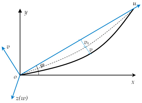
Figure 1. Calculation diagram of the cable.

The conversion formulations of the two coordinate systems are given in Equation (1).

$$\{\begin{array}{c}u=ysin\phi +xcos\phi \\ v=ycos\phi -xsin\phi \\ w=z\end{array}$$

(1)

To derive the vibration equations of the cable, four basic assumptions are given [23]:

• The bending and torsional stiffness of the cable are ignored;
• The density of the cable remains constant along the u-axis;
• The stress of the cable is always within the elastic limit;
• The initial curve of the sagged cable is approximated as a parabola.

The first assumption is made under the consideration that the length of the cable is much larger than its diameter, and its slenderness ratio is usually less than 0.001 for the long-span cable-stayed bridge. The third assumption holds for the long-span bridge because the cable material is high-strength structural steel with an ultimate tensile strength of over 1570 megapascals. The cables’ stresses during service are usually within one-third of the ultimate tensile strength. It should be noticed that the boundary conditions of the cable are the pure force boundary conditions, which means the cable is under the control of the force on its two ends. Based on these assumptions above, the force analysis of the cable’s microsegment can be conducted in the u-v-w coordinate system, as shown in Figure 2.

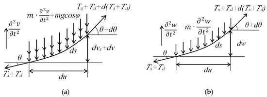
Figure 2. Force analysis of cable’s microsegment: (a) in-plane diagram; (b) out-plane diagram.

The partial differential equations can be derived based on D’Alembert’s principle [24], as shown in Equation (2).

$$\{\begin{array}{c}\frac{\partial }{\partial s}\left[\left(T_s+T_d\right)·\frac{\partial \left(v_s+v\right)}{\partial s}\right]=m·\frac{{\partial }^{2}v}{\partial t^2}+c_v·\frac{\partial v}{\partial t}+mgcos\phi +f_v\left(u,t\right)\\ \frac{\partial }{\partial s}\left[\left(T_s+T_d\right)·\frac{\partial w}{\partial s}\right]=m·\frac{{\partial }^{2}w}{\partial t^2}+c_w·\frac{\partial w}{\partial t}+f_w\left(u,t\right) \end{array}$$

(2)

where T_s is the initial tension; T_d is the tension caused by the cable vibration; v_s is the initial sag; c_v and c_w are the in-plane and out-plane damping coefficients; f_v(u, t) and f_w(u, t) are the in-plane and out-plane exciting forces; and m is the linear density of the cable.

Assuming that the initial arc length of the microsegment is ds₀, and it becomes ds during the cable vibration, then the two arc lengths can be expressed as Equations (3) and (4), respectively, by ignoring the axial deformation:

$$d{s}_0^2=d{u}^2+d{v}_s^2$$

(3)

$$d{s}^2=d{u}^2+{\left(d{v}_s+dv\right)}^2+d{w}^2$$

(4)

Then, the dynamic strain of the cable can be deduced as Equation (5).

$$\begin{gathered} \mathsf{\epsilon }=\frac{ds-d{s}_0}{d{s}_0}=\frac{\sqrt{d{u}^2+{\left(d{v}_s+dv\right)}^2+d{w}^2}-d{s}_0}{d{s}_0} \\ =\frac{\sqrt{d{s}_0^2+2dvd{v}_s+d{v}^2+d{w}^2}-d{s}_0}{d{s}_0} \\ \approx \frac{dv}{d{s}_0}\frac{d{v}_s}{d{s}_0}+\frac{1}{2}\left[{\left(\frac{dv}{d{s}_0}\right)}^2+{\left(\frac{dw}{d{s}_0}\right)}^2\right] \end{gathered}$$

(5)

The dynamic tension T_d can be decomposed into two components: the dynamic tension T_v resulting from cable vibration-induced deformation and the dynamic tension T_m arising from changes in the boundary conditions of the cable. During cable vibration, a relationship exists between the force acting on each micro-segment of the cable and its horizontal component force, as in Equation (6).

$$\frac{T}{T_v}=\frac{ds}{du}$$

(6)

where T = EAε is the axial force of the cable.

Then, the dynamic tension T_v can be derived as Equation (7).

$$T_v\frac{ds}{du}{\left(\frac{d{s}_0}{du}\right)}^2=EA\left\{\frac{dv}{du}\frac{d{v}_s}{du}+\frac{1}{2}\left[{\left(\frac{dv}{du}\right)}^2+{\left(\frac{dw}{du}\right)}^2\right]\right\}$$

(7)

The approximate average dynamic tension can be obtained by integrating Equation (7) along the u-axis for the entire cable.

$$T_v=\frac{EA}{l_v}\left\{{{\displaystyle \int }}_0^l\left[\frac{dv}{du}\frac{d{v}_s}{du}+\frac{1}{2}\left({\left(\frac{dv}{du}\right)}^2+{\left(\frac{dw}{du}\right)}^2\right)\right]du\right\}$$

(8)

where l_v is the in-plane virtual length.

$$l_v={{\displaystyle \int }}_0^l\frac{ds}{du}{\left(\frac{d{s}_0}{du}\right)}^{2}du={{\displaystyle \int }}_0^l\sqrt{1+\frac{d^{2}v}{d{u}^2}}·\left(1+\frac{d^2{v}_s}{d{u}^2}\right)du$$

(9)

The out-plane dynamic tension T_w can be derived analogically, and it should be noted that there is no out-plane sag.

$$T_w=\frac{EA}{l_w}\left\{{{\displaystyle \int }}_0^l\frac{1}{2}\left({\left(\frac{dv}{du}\right)}^2+{\left(\frac{dw}{du}\right)}^2\right)du\right\}$$

(10)

where l_w is the out-plane virtual length.

$$l_w={{\displaystyle \int }}_0^l\frac{ds}{du}du={{\displaystyle \int }}_0^l\sqrt{1+\frac{d^{2}v}{d{u}^2}}du$$

(11)

The dynamic tension caused by the variation of the boundary condition is deduced using Equation (12).

$$\begin{gathered} T_m=\frac{EA}{l}\left(\sqrt{{\left(l+\Delta U\right)}^2+\Delta V^2+\Delta W^2}-l\right) \\ \approx \frac{EA}{l}\Delta U\left(t\right)+EA\frac{\Delta U^2\left(t\right)}{2l^2}+EA\frac{\Delta V^2\left(t\right)}{2l^2}+EA\frac{\Delta W^2\left(t\right)}{2l^2} \end{gathered}$$

(12)

The variation of the boundary condition is the relative displacement of the cable’s two ends, which is relatively small compared to the length of the cable, so the high-order terms in Equation (12) can be ignored to simplify the equation as Equation (13).

$$T_m=\frac{EA}{l}\Delta U\left(t\right)$$

(13)

Assuming the force excitation of the cable caused by the end vibration is a linear triangular distribution along the axis of the cable, the force in-plane and out-plane excitation can be deduced as Equations (14) and (15).

$$f_v\left(u,t\right)=m\left(\frac{x}{l}{\ddot{V}}_j+\left(1-\frac{x}{l}\right)\ddot{V_i}\right)$$

(14)

$$f_w\left(w,t\right)=m\left(\frac{x}{l}{\ddot{W}}_j+\left(1-\frac{x}{l}\right)\ddot{W_i}\right)$$

(15)

Substituting Equation (3) to Equation (15) into Equation (2), the partial differential equations of the cable’s in-plane and out-plane can be rewritten as:

$$\begin{array}{c}\left\{T_s+\frac{EA}{l}\Delta U\left(t\right)+\frac{EA}{l_v}\left\{{{\displaystyle \int }}_0^l\left[\frac{dv}{du}\frac{d{v}_s}{du}+\frac{1}{2}\left({\left(\frac{dv}{du}\right)}^2+{\left(\frac{dw}{du}\right)}^2\right)\right]du\right\} \right\}\frac{d^{2}v}{d{u}^2}+\\ \left\{\frac{EA}{l_v}\left\{{{\displaystyle \int }}_0^l\left[\frac{dv}{du}\frac{d{v}_s}{du}+\frac{1}{2}\left({\left(\frac{dv}{du}\right)}^2+{\left(\frac{dw}{du}\right)}^2\right)\right]du\right\}\right\}\frac{d^2{v}_s}{d{u}^2}=m\ddot{v}+c_v\dot{v}+mgcos\phi +m\left(\frac{x}{l}{\ddot{V}}_j+\left(1-\frac{x}{l}\right)\ddot{V_i}\right)\end{array}$$

(16)

$$\left\{T_s+\frac{EA}{l}\Delta U\left(t\right)+\frac{EA}{l_w}\left\{{{\displaystyle \int }}_0^l\frac{1}{2}\left({\left(\frac{dv}{du}\right)}^2+{\left(\frac{dw}{du}\right)}^2\right)du\right\} \right\}\frac{d^{2}w}{d{u}^2}=m\ddot{w}+c_w\dot{w}+m\left(\frac{x}{l}{\ddot{W}}_j+\left(1-\frac{x}{l}\right)\ddot{W_i}\right)$$

(17)

The Galerkin method [25] is adopted to solve the partial differential equations, considering that the vibration of the cable is the superposition of the first m-order sinusoidal modes.

$$v\left(u,t\right)={\displaystyle \sum }_{k=1}^m{V}_k\left(t\right)·\sin \left(\frac{k\pi u}{l}\right)$$

(18)

$$w\left(u,t\right)={\displaystyle \sum }_{k=1}^m{W}_k\left(t\right)·\sin \left(\frac{k\pi u}{l}\right)$$

(19)

Ignoring the variation in the damping ratio for the cable, the nth order in-plane and out-plane vibration equations of the cable can be derived:

$${\ddot{V}}_n+2\xi {\omega }_{vn}{\dot{V}}_n+{\omega }_{vn}^2{V}_n+{\alpha }_1{V}_n+{\alpha }_2{V}_n^2+{\alpha }_3{V}_n^3+{\alpha }_4{W}_n^2+{\alpha }_5{V}_n{W}_n^2+A={\alpha }_6$$

(20)

$${\ddot{W}}_n+2\xi {\omega }_{wn}{\dot{W}}_n+{\omega }_{wn}^2{W}_n+{\beta }_1{W}_n+{\beta }_2{W}_n^2+{\beta }_3{W}_n{V}_n^2+B={\beta }_4$$

(21)

2.2. Model Verification

The longest cable of a rail-cum-road cable-stayed bridge, whose length, inclination angle, elastic modulus, linear density, initial tension, and cross-sectional area are 295.995 m, 25 degrees, 2 × 10¹¹ pascals, 153.55 kg per meter, 9438 kilonewtons, 0.01828 square meters, respectively, was taken as the prototype. The cable was simulated using 60 link180 elements in ANSYS software. The link180 element is a three-dimensional uniaxial bar element with a tension-only capacity, which is useful for modeling the cable’s properties. A form-finding analysis [26] was first executed to obtain the initial shape of the cable under the action of initial tension and gravity, as shown in Figure 3. The form-finding analysis should be performed first because the gravity of the cable will generate an initial sag, which is considered for accurate simulation purposes. Then, the first four modal frequencies of the cable, which are compared with the numerical model results in Table 1, can be obtained by conducting a linear perturbation modal analysis with prestress [27]. The linear perturbation method is commonly used to solve a linear problem with a preloaded status. After conducting a linear perturbation analysis, the tangent stiffness matrix of the preloaded structure can be gained, which will be used for the subsequent modal analysis.

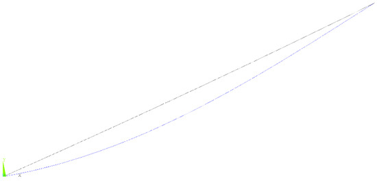
Figure 3. FEM of the cable.

Table 1. Comparison of the first four modal frequencies.

Order	FEM Results (Hz)		Numerical Model Results (Hz)		Errors
	In-Plane	Out-Plane	In-Plane	Out-Plane	In-Plane	Out-Plane
1	0.43098	0.41902	0.43081	0.41879	0.0%	0.1%
2	0.83822	0.83831	0.83759	0.83759	0.1%	0.1%
3	1.25859	1.25818	1.25683	1.25638	0.1%	0.1%
4	1.67887	1.67892	1.67518	1.67518	0.2%	0.2%

The comparison results of the first four modal frequencies of the cable demonstrate a high level of agreement between the finite element model and the numerical model, thus confirming the accuracy and validity of the numerical model. Only the first four modal frequencies are compared because the cable’s n-th frequency is approximately n times the fundamental frequency, so comparing the higher frequencies is redundant.

3. Numerical Simulation of the Rail-Cum-Road Cable-Stayed Bridge

The Huanggang Yangtze River bridge was used as the prototype bridge. This is a cable-stayed bridge with a steel truss girder and two pylons and has a semi-floating system. The main girder consists of double bridge decks, four-lane highways with a design speed of 100 km per hour for the upper layer, and two-track high-speed railways with a 200 km per hour design speed for the sublayer. The bridge’s total length is 1218.5 m, and the main span is 567 m; the span configuration is shown in Figure 4. The main bridge is supported by two sliding bearings at each of the side piers, auxiliary piers, and pylons, with the upstream side bearing restraining the vertical displacement degrees of freedom, the downstream side bearing restraining the vertical and transverse displacement degrees of freedom, and four longitudinal viscous dampers installed at each pylon.

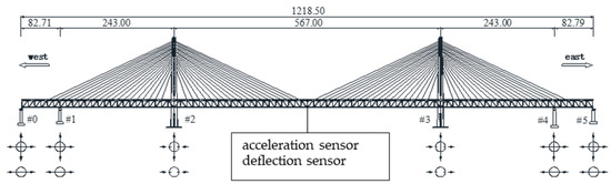
Figure 4. Front elevation of the bridge (units: meters).

A long-span rail-cum-road cable-stayed bridge is subjected to the combined action of wind, trains, vehicles, and environmental temperatures during its operation period [28], and the long-term mechanical properties of the steel truss girders, cables, and pylons are worthy of attention during the service period under these loads. To accurately simulate the dynamic and static mechanical behavior of the bridge, a fine finite element model was established based on the ANSYS software [29], as shown in Figure 5, in which the steel trusses, the longitudinal and transverse ribs of the orthotropic anisotropic deck, were simulated using BEAM188 elements, the deck slabs were simulated using SHELL181 elements, the cables were simulated using LINK180 elements, and the concrete pylons were simulated using SOLID65 elements. These elements are recommended by the users’ guide documentation of ANSYS software to simulate slender to moderately stubby/thick beam structures, thin to moderately thick shell structures, sagging cables, and solids with or without reinforcing bars, respectively. There are 41,268 nodes and 125,508 elements, of which 25,994 are beam elements, 11,902 are shell elements, 152 are link elements, and 87,460 are solid elements. The size for beam and shell elements is within the range of 1.7 to 7.4 m, while for solid elements, they fall within the range of 1.2 to 4.2 m, as listed in Table 2, and the force and displacement convergence criteria are adopted and controlled by the default settings of the solver.

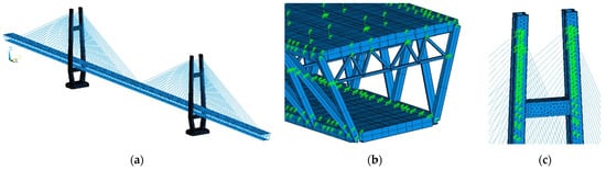
Figure 5. FEM of the bridge: (a) the whole bridge; (b) the steel truss beam; and (c) the pylon.

Table 2. Element summaries.

Element Type	Amounts	Element Size (Meters)
BEAM188	25,994	1.7~7.4
SHELL181	11,902	1.7~7.4
LINK180	152	/
SOLID65	87,460	1.2~4.2

The material of the steel truss girder was a high-strength structural steel with a yield strength of 390 Mpa. The connections among the deck slabs simulated by shell elements and the longitudinal and transverse ribs simulated by beam elements were processed by coupling their degrees of freedom. The initial strain method was adopted to add initial tension to the cables, and the degrees of freedom of the two end nodes of the cable simulated by the link element were coupled to its vicinal nodes of the solid elements and beam elements. The nonlinear geometrical effects were considered by turning on the large deflection effects during the analysis period.

Four fluid viscous dampers were installed between the main girder and crossbeam of the pylons to decrease the longitudinal vibration of the girder caused by earthquakes, winds, vehicles, and trains.

The fluid viscous damper is a kind of velocity-dependent damper, and the damping force is only related to the relative velocity between its two end nodes, so it did not provide additional stiffness to the whole structure. The damping force, velocity exponent, and damping coefficient of the damper adopted were 3000 kilonewtons, 0.25, and 3998 kilonewton seconds per meter, respectively.

The COMBIN37 element in the ANSYS software can simulate the fluid viscous damper, a unidirectional element with nonlinear capacity, as shown in Figure 6. The element is defined by two pairs of nodes: active nodes I and J, which determine the element’s position, and optional control nodes K and J, which are used to control the nonlinear behavior of the element. The two pairs of nodes can have inconsistent degrees of freedom. Each has only one degree of freedom: a translation in a nodal coordinate direction, rotation about a nodal coordinate axis, pressure, or temperature.

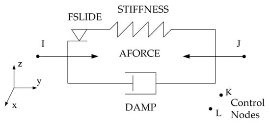
Figure 6. COMBIN37 geometry.

To simulate the behavior of the fluid viscous damper, the key options of the COMBIN37 element should be set as follows:

• The first key option, KEYOPT(1), should be set as 2 to allow the control parameter to be the relative velocity of the two control nodes, K and L;
• Both the fourth key option KEYOPT(4) and the fifth key option KEYOPT(5) should be set as 1 to allow the element to always be activated;
• The sixth key option, KEYOPT(6), should be set as 2 to correct the damping parameter.

The rest of the key options are set as defaults, and the damping parameter of the element is corrected as Equation (22).

$$D=C_0+C_1{\left|P\right|}^{C_2}+C_3{\left|P\right|}^{C_4}$$

(22)

where C₀ is the initial damping coefficient set by the second real constant, C₁ to C₄ are the ninth to twelfth real constants, and P is the control parameter set by the second key option. By setting the real constants C₀, C₃, and C₄ as zero and letting the control nodes K and J be coincident with the active nodes I and J, the damping force of the element can be corrected to Equation (23).

$$F=\left(C_0+C_1{\left|P\right|}^{C_2}+C_3{\left|P\right|}^{C_4}\right)·\left|v\right|·\mathrm{sgn}\left(v\right)=C_1{\left|v\right|}^{1+C_2}\mathrm{sgn}\left(v\right)$$

(23)

where v is the relative velocity of the active nodes I and J, and sgn is the sign function.

Equation (23) is similar to the mechanics model of the standard velocity-dependent damper shown in Equation (24).

$$F=C{\left|v\right|}^n\mathrm{sgn}(v)$$

(24)

where C is the damping coefficient and n is the velocity index.

It can be seen from Equations (23) and (24) that the ninth real constant, C₁, should be set as the damping coefficient, and the tenth real constant, C₂, should be set as the velocity index minus one.

4. The Dynamic Behavior of the Cable under the Action of the Train

To simplify the analysis and save computing resources, the moving loads method [30] that simplifies the train to several concentration forces applied on the bridge was adopted to simulate the train driving through the bridge. The train prototype was the CRH3 electric multiple unit (EMU), consisting of eight carriages [31]. An empty EMU weighs 380 tons, and an EMU has a seating capacity of 601 people. Assuming that the average weight per person is 80 kg (People’s Republic of China Ministry of Railways 2001), each carriage’s weight is G = 53,510 kg. Because one carriage is supported by eight wheels, the load model of the carriage is divided into eight point loads, so the vertical excitation force generated by a wheel is F = G/8 × 9.8 N/kg = 65,549.75 N [32]. The moving loads of two EMUs with 16 carriages are grouped as 16 × 8 × F. The train load is shown in Figure 7.

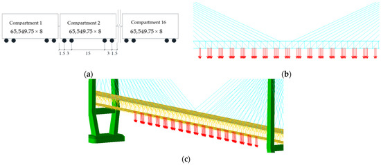
Figure 7. The moving load applied on the bridge: (a) the train model; (b) the local moving load diagram; and (c) the whole moving load diagram.

The bridge was equipped with a structural health monitoring (SHM) system, which was detailed in reference [28], and the data recorded by the displacement sensors and acceleration sensors installed at the midspan of the main span near the downstream side could be used to verify the accuracy of the FEM. The comparison of the deflection and acceleration temporal curves between the monitoring data and simulated data is shown in Figure 8 and Table 3. It could be found that the deflection data from the FEM simulation was coincident with that from the SHM system, and neither of them showed obvious vibration characteristics. For the acceleration result, the simulated data were much smaller than the monitoring data at the beginning and end stages, but there was little difference after the train drove to the main span. This may have been caused by ignoring the wind influence during the simulation. The analysis above indicates that the FEM is accurate enough to simulate the real bridge, and the moving loads method is meaningful in this research.

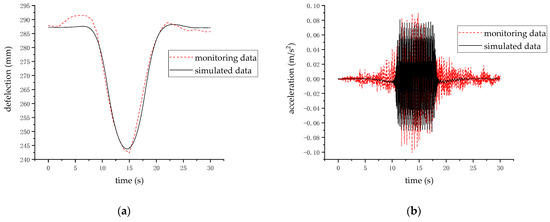
Figure 8. Comparison between the monitoring and simulated data: (a) deflections; (b) accelerations.

Table 3. Comparison between the monitoring data and simulated data.

Types	Monitoring Data		Simulated Data		Errors
	Maximum	Minimum	Maximum	Minimum	Maximum	Minimum
Deflection (mm)	291.52	242.33	288.21	243.76	1.1%	0.6%
Acceleration (mm/s2)	0.090	−0.101	0.081	−0.072	10.0%	28.6%

Considering the symmetry of the bridge, only the load case where the train drives from the west side to the east side on the downstream tracks was analyzed. The spatial distribution of the extreme value of the displacements and accelerations at the connection of the beam and cables for each of the 38 cables on the upstream and downstream sides near the west side is given in Figure 9. The amplitude of the displacements under the moving loads was taken as the difference between the initial deflection and the minimum value of the deflection temporal curves.

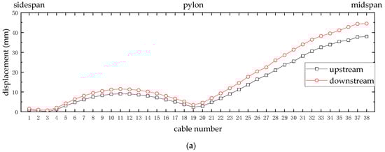
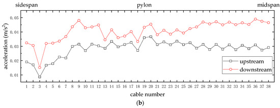
Figure 9. The spatial distribution of the extreme value: (a) displacements; (b) accelerations.

It could be found that the deflection and acceleration amplitudes near the train driving side were larger than those away from it, but the trends of both curves were similar. The maximum value of displacement amplitude occurred at the longest cable near the middle of the main span (No. 38). The cable at the side span of the bridge was relatively less affected by the train load, mainly because the side span was shorter than the main span. Thus, the bridge deflection was smaller under the train load, and this phenomenon could also be verified by the data from the bridge’s SHM system, which were analyzed by Ding et al. [28]. The acceleration amplitude from the bridge bank to the middle of the side span showed a trend of gradual increase. In contrast, the change from the middle of the side span to the middle of the main span was not significant, mainly because the train had not yet wholly entered the bridge at the beginning; the amplitude of the vibration generated by the train gradually increased along with the train entering the bridge and tended to be stable after the train had fully entered the bridge.

The amplitude of displacement and acceleration was higher at the connection between the cable and the main girder near the side where the train load was located. This was primarily because the train loads were eccentric, causing them to act on the main girder unevenly. Consequently, the structures near the train side were subjected to higher forces, resulting in more significant vibrations.

5. Vibration Analysis of the Cable under Double-End Excitation

The partial differential equations derived for the cable vibration under the double-end excitation were numerically solved using MATLAB software. The displacement and acceleration time history of the cable endpoint extracted from the moving load analysis by the finite element were input into the MATLAB solution program as the cable end excitation, and all orders vibration of the cable could be obtained. The vibration of any cable point could be derived by adding the cable’s first six-order vibration, which was accurate enough. It is important to note that higher-order vibrations only contributed to an insignificant extent, within 1%. Therefore, their impact can be considered negligible when evaluating the overall performance.

The comparison of the displacement time history between the input end excitation and the vibration of the midpoint of the No. 38 cable, considering the first order, the first three order, and first six order vibrations of the cable, is shown in Figure 10. It can be seen that the input displacement excitation at the end of the cable was amplified by a factor of nearly two and would cause irregular vibrations of the cable simultaneously. The frequency of the forced vibration of the cable was close to the excitation frequency, so it is necessary to keep the frequency of the dynamic excitation generated by the passing train away from the fundamental frequency of the cable to avoid resonance.

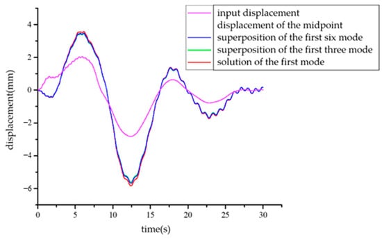
Figure 10. The displacement time history of the end excitation and midpoint of the cable.

6. Conclusions

An accurate FEM with a relative error of about 1% for deflection and 29% for acceleration compared with the data from the SHM system in modeling a train passing case of a rail-cum-road cable-stayed bridge was established based on the ANSYS software to analyze the vibration behavior of the bridge and the cable. To comprehend the vibration behavior of the cable under the double-end excitations, the partial differential equations were derived by neglecting the bending stiffness and numerically solved using MATLAB software [33]. The moving loads method was adopted to simulate the train, and the cable vibration under the action of train loads was analyzed in detail. Some conclusions can be summarized, as follows:

• The cable will generate parametric vibration under the end axial displacement excitation and forced vibration under the end vertical displacement excitation. The numerical vibration model established through simplifying the two forms of excitation agreed well with the multi-segment rod finite element model analysis results by less than 1% relative errors for its first four frequencies. In practical applications, the numerical model is more straightforward to use than the finite element model and can quickly calculate the vibration response of any position of the cable for the symmetrical bridge structures;
• Under the action of the high-speed train, the displacement and acceleration amplitude of the cable near the train load side were larger; the maximum displacement amplitude appeared on the longest cable near the middle of the main span, and the acceleration amplitude of the cable in the main span was almost the same; and the cables on the side spans of the bridge were relatively less affected by the train load;
• While high-speed trains pass over the bridge with a velocity of over 200 km per hour, the excitation generated on the cable end will make the cable vibrate, and the cable vibration frequency will be close to the dynamic frequency excited by the train wheel. Therefore, it is necessary to avoid the train passing over the bridge at certain velocities to avoid cable resonance.
• As the PDEs of the cable vibration were derived with four assumptions, the numerical model in this paper can be only used for slender cables on which the bending and torsional stiffness can be ignored. Further work will be conducted on the fatigue assessment of the cable based on its vibration character studies in this paper.

References

- Liu, Z.; Guo, T.; Yu, X.; Huang, X.; Correia, J. Corrosion fatigue and electrochemical behaviour of steel wires used in bridge cables. Fatigue Fract. Eng. Mater. Struct. 2021, 44, 63–73. [Google Scholar] [CrossRef]
- Zhang, Z.; Guo, T.; Liu, Z.; Wang, S. Test and Analysis of Postfire Fatigue Performance of Steel Wires and Cables. J. Bridge Eng. 2022, 27, 04022096. [Google Scholar] [CrossRef]
- Li, Y.Q.; Zhao, H.W.; Yue, Z.X.; Li, Y.W.; Zhang, Y.; Zhao, D.C. Real-Time Intelligent Prediction Method of Cable’s Fundamental Frequency for Intelligent Maintenance of Cable-Stayed Bridges. Sustainability 2023, 15, 4086. [Google Scholar] [CrossRef]
- Zhao, H.; Ding, Y.; Li, A.; Chen, B.; Zhang, X. State-monitoring for abnormal vibration of bridge cables focusing on non-stationary responses: From knowledge in phenomena to digital indicators. Measurement 2022, 205, 112148. [Google Scholar] [CrossRef]
- Fang, Z.; Ding, Y.; Wei, X.; Li, A.; Geng, F. Fatigue failure and optimization of double-sided weld in orthotropic steel bridge decks. Eng. Fail. Anal. 2020, 116, 104750. [Google Scholar] [CrossRef]
- Gao, Z. Major Steel Bridges for High Speed Railway in China. In Bridge Maintenance, Safety, Management and Life-Cycle Optimization—Proceedings of the 5th International Conference on Bridge Maintenance, Safety and Management; Advanced Technology for Large Structural Systems (ATLSS) Engineering Research Center: Philadelphia, PA, USA, 2010. [Google Scholar]
- Ge, Y.; Zhao, L.; Cao, J. Case study of vortex-induced vibration and mitigation mechanism for a long-span suspension bridge. J. Wind. Eng. Ind. Aerodyn. 2022, 220, 104866. [Google Scholar] [CrossRef]
- Li, Y.; Qiang, S.; Liao, H.; Xu, Y. Dynamics of wind–rail vehicle–bridge systems. J. Wind. Eng. Ind. Aerodyn. 2005, 93, 483–507. [Google Scholar] [CrossRef]
- Nassiraei, H.; Zhu, L.; Gu, C. Static capacity of collar plate reinforced tubular X-connections subjected to compressive loading: Study of geometrical effects and parametric formulation. Ships Offshore Struct. 2021, 16, 54–69. [Google Scholar] [CrossRef]
- Chen, C.-C.; Wu, W.-H.; Chen, S.-Y.; Lai, G. A novel tension estimation approach for elastic cables by elimination of complex boundary condition effects employing mode shape functions. Eng. Struct. 2018, 166, 152–166. [Google Scholar] [CrossRef]
- Bonopera, M.; Chang, K.-C.; Tullini, N. Vibration of prestressed beams: Experimental and finite-element analysis of post–tensioned thin-walled box-girders. J. Constr. Steel Res. 2023, 205, 107854. [Google Scholar] [CrossRef]
- Yao, Y.; Xu, B.; Wang, Y. Research on the Train-Bridge Coupled Vibration and Dynamic Performance of Steel Box Hybrid Girder Cable-Stayed Railway Bridge. Teh. Vjesn.—Tech. Gaz. 2020, 27, 656–664. [Google Scholar] [CrossRef]
- Wu, J.; Cai, C.; Li, X.; Liu, D. Dynamic analysis of train and bridge in crosswinds based on a coupled wind-train-track-bridge model. Adv. Struct. Eng. 2023, 26, 904–919. [Google Scholar] [CrossRef]
- Le, L.X.; Siringoringo, D.M.; Katsuchi, H.; Fujino, Y. Stay cable tension estimation of cable-stayed bridge under limited information on cable properties using artificial neural networks. Struct. Control. Health Monit. 2022, 29, e3015. [Google Scholar] [CrossRef]
- Wang, S.; Luo, J.; Zhu, S.; Han, Z.; Zhao, G. Random dynamic analysis on a high-speed train moving over a long-span cable-stayed bridge. Int. J. Rail Transp. 2022, 10, 331–351. [Google Scholar] [CrossRef]
- Wu, Y.; Zhou, J.; Zhang, J.; Wen, Q.; Li, X. Train-Bridge Dynamic Behaviour of Long-Span Asymmetrical-Stiffness Cable-Stayed Bridge. Shock. Vib. 2021, 2021, 1–15. [Google Scholar] [CrossRef]
- Kim, S.; Lee, S.-H.; Kim, S. Pointwise multiclass vibration classification for cable-supported bridges using a signal-segmentation deep network. Eng. Struct. 2023, 279, 115599. [Google Scholar] [CrossRef]
- Górski, P.; Tatara, M.; Stankiewicz, B. Vibration serviceability of all-GFRP cable-stayed footbridge under various service excitations. Measurement 2021, 183, 109822. [Google Scholar] [CrossRef]
- Liu, D.; Li, X.; Mei, F.; Xin, L.; Zhou, Z. Effect of vertical vortex-induced vibration of bridge on railway vehicle’s running performance. Veh. Syst. Dyn. 2023, 61, 1432–1447. [Google Scholar] [CrossRef]
- Gong, W.; Zhu, Z.; Liu, Y.; Ruitao, L.; Yongjiu, T.; Lizhong, J. Running safety assessment of a train traversing a three-tower cable-stayed bridge under spatially varying ground motion. Railw. Eng. Sci. 2020, 28, 184–198. [Google Scholar] [CrossRef]
- Zeng, Y.; Yu, H.; Tan, Y.; Tan, H.; Zheng, H. Dynamic Characteristics of a Double-Pylon Cable-Stayed Bridge with Steel Truss Girder and Single-Cable Plane. Adv. Civ. Eng. 2021, 2021, 1–15. [Google Scholar] [CrossRef]
- Gong, W.; Zhu, Z.; Wang, K.; Yang, W.; Bai, Y.; Ren, J. A real-time co-simulation solution for train–track–bridge interaction. J. Vib. Control. 2021, 27, 1606–1616. [Google Scholar] [CrossRef]
- Wang, T.; Shen, R. Research on Characteristics of Cable-beam Vibration of Railway Cable-stayed Bridge under Train Load. J. Archit. Civ. Eng. 2015, 32, 92–101. (In Chinese) [Google Scholar]
- Slate, F. The Essential Meaning of d’Alembert’s Principle. Science 1908, 28, 154–157. [Google Scholar] [CrossRef] [PubMed][Green Version]
- Douglas, J.J.; Dupont, T. Galerkin Methods for Parabolic Equations. SIAM J. Numer. Anal. 1970, 7, 575–626. [Google Scholar] [CrossRef]
- Zhao, Z.; Yu, D.; Zhang, T.; Zhang, N.; Liu, H.; Liang, B.; Xian, L. Efficient form-finding algorithm for freeform grid structures based on inverse hanging method. J. Build. Eng. 2022, 46, 103746. [Google Scholar] [CrossRef]
- Liu, Y.; Guo, K.; Wang, C.; Gao, H. Wrinkling and ratcheting of a thin film on cyclically deforming plastic substrate: Mechanical instability of the solid-electrolyte interphase in Li–ion batteries. J. Mech. Phys. Solids 2019, 123, 103–118. [Google Scholar] [CrossRef]
- Zhao, H.; Ding, Y.; Meng, L.; Qin, Z.; Yang, F.; Li, A. Bayesian Multiple Linear Regression and New Modeling Paradigm for Structural Deflection Robust to Data Time Lag and Abnormal Signal. IEEE Sens. J. 2023, 23, 19635–19647. [Google Scholar] [CrossRef]
- ANSYS Mechanical, Release 2019: User’s Guide. Help System, User’s Guides, ANSYS, Inc. 2019. Available online: https://ansyshelp.ansys.com/ (accessed on 4 October 2022).
- Koh, C.; Chiew, G.; Lim, C. A numerical method for moving load on continuum. J. Sound Vib. 2007, 300, 126–138. [Google Scholar] [CrossRef]
- Sun, Z.; Zhang, Y.; Guo, D.; Yang, G.; Liu, Y. Research on Running Stability of CRH3 High Speed Trains Passing by Each Other. Eng. Appl. Comput. Fluid Mech. 2014, 8, 140–157. [Google Scholar] [CrossRef]
- Zhao, H.W.; Ding, Y.L.; An, Y.H.; Li, A.Q. Transverse Dynamic Mechanical Behavior of Hangers in the Rigid Tied-Arch Bridge under Train Loads. J. Perform. Constr. Facil. -ASCE 2017, 31, 04016072. [Google Scholar] [CrossRef]
- MathWorks Math. Graphics. Programming. 2022. Available online: https://www.mathworks.com/products/matlab.html (accessed on 19 September 2022).
Disclaimer/Publisher’s Note: The statements, opinions and data contained in all publications are solely those of the individual author(s) and contributor(s) and not of MDPI and/or the editor(s). MDPI and/or the editor(s) disclaim responsibility for any injury to people or property resulting from any ideas, methods, instructions or products referred to in the content. |
© 2023 by the authors. Licensee MDPI, Basel, Switzerland. This article is an open access article distributed under the terms and conditions of the Creative Commons Attribution (CC BY) license (https://creativecommons.org/licenses/by/4.0/).