Ultraviolet Erythemal Irradiance (UVER) under Different Sky Conditions in Burgos, Spain: Multilinear Regression and Artificial Neural Network Models

Abstract

Different strategies for modeling Global Horizontal UltraViolet Erythemal irradiance ($\mathrm{G}\mathrm{H}\mathrm{U}\mathrm{V}\mathrm{E}$) based on meteorological parameters measured in Burgos (Spain) have been developed. The experimental campaign ran from September 2020 to June 2022. The selection of relevant variables for modeling was based on Pearson’s correlation coefficient. Multilinear Regression Model $\left(\mathrm{M}\mathrm{L}\mathrm{R}\right)$ and artificial neural network $\left(\mathrm{A}\mathrm{N}\mathrm{N}\right)$ techniques were employed to model $\mathrm{G}\mathrm{H}\mathrm{U}\mathrm{V}\mathrm{E}$ under different sky conditions (all skies, overcast, intermediate, and clear skies), classified according to the $\mathrm{C}\mathrm{I}\mathrm{E}$ standard on a 10 min basis. $\mathrm{A}\mathrm{N}\mathrm{N}$ models of $\mathrm{G}\mathrm{H}\mathrm{U}\mathrm{V}\mathrm{E}$ outperform those based on MLR according to the traditional statistical indices used in this study (${\mathrm{R}}^2$, $\mathrm{M}\mathrm{B}\mathrm{E}$, and $\mathrm{n}\mathrm{R}\mathrm{M}\mathrm{S}\mathrm{E}$). Moreover, the work proposes a simple all-sky $\mathrm{A}\mathrm{N}\mathrm{N}$ model of $\mathrm{G}\mathrm{H}\mathrm{U}\mathrm{V}\mathrm{E}$ based on usually recorded variables at ground meteorological stations.

1. Introduction

Ultraviolet radiation $\left(\mathrm{U}\mathrm{V}\right)$ represents a small fraction of total solar radiation (5–7%) [1]. It is a highly energetic component of the solar spectrum that must be monitored as it can be detrimental to life on Earth [2], becoming the main risk factor for human health among photo-biological factors [3]. The UV region of the solar spectrum spans wavelengths between 100 and 400 nm, and it is divided into three components, i.e., $\mathrm{U}\mathrm{V}\mathrm{A}$, $\mathrm{U}\mathrm{V}\mathrm{B},$ and $\mathrm{U}\mathrm{V}\mathrm{C}$. Although $\mathrm{U}\mathrm{V}\mathrm{C}$ radiation (100–280 nm) is entirely absorbed by atmospheric oxygen and ozone, a fraction of $\mathrm{U}\mathrm{V}\mathrm{B}$ (280–315 nm) and $\mathrm{U}\mathrm{V}\mathrm{A}$ (315–400 nm) reaches the Earth’s surface as ozone partially absorbs these wavelengths [4]. Surface $\mathrm{U}\mathrm{V}$ is also influenced by geographical parameters like altitude over the sea level and latitude [5].

$\mathrm{U}\mathrm{V}$ radiation exerts significant effects on biological and photochemical processes [6], showing both beneficial and detrimental impacts. It has beneficial effects on humans, animals, plants, and the biosphere: while moderate doses of $\mathrm{U}\mathrm{V}$ radiation enhance vitamin D synthesis, promote mental health, and reduce blood pressure [3,7,8], excessive exposure to $\mathrm{U}\mathrm{V}$ radiation can cause cataracts, premature aging of the skin and skin cancer [1,9,10,11]. It also has negative effects on organisms, marine and terrestrial ecosystems, and certain building materials (paints and plastics) [12,13]. Ideally, there should be a balance in $\mathrm{U}\mathrm{V}$ radiation exposure to reduce the adverse effects associated with too few or too high exposures [8].

The impacts of $\mathrm{U}\mathrm{V}$ radiation on the skin have been commonly assessed using $\mathrm{U}\mathrm{V}$ erythemal irradiance ($\mathrm{U}\mathrm{V}\mathrm{E}\mathrm{R}$). In accordance with the $\mathrm{I}\mathrm{S}\mathrm{O}/\mathrm{C}\mathrm{I}\mathrm{E}17166:2019\left(\mathrm{E}\right)$ standard [14], $\mathrm{U}\mathrm{V}\mathrm{E}\mathrm{R}$ is determined by applying a spectral weighting function known as the erythema spectral weighting function. This function quantifies the effectiveness of radiation at each wavelength $\left(\mathsf{\lambda }\right)$ to cause minimal erythema. The $\mathrm{U}\mathrm{V}\mathrm{E}\mathrm{R}$ value is obtained by weighting the spectral irradiance of the $\mathrm{U}\mathrm{V}$ radiation at each wavelength using the corresponding erythema effectiveness factor and then summing up these weighted values for all wavelengths present in the source spectrum, as specified in the standard.

Due to the lack of $\mathrm{U}\mathrm{V}$ and $\mathrm{U}\mathrm{V}\mathrm{E}\mathrm{R}$ sensors in many ground-based weather stations [15], these variables are often estimated from other radiometric or meteorological parameters. The effect of cloudiness on $\mathrm{U}\mathrm{V}\mathrm{E}\mathrm{R}$ has been analyzed for all-sky conditions. In overcast conditions and skies with low clouds, $\mathrm{U}\mathrm{V}\mathrm{E}\mathrm{R}$ decreases as cloudiness increases [16]. Cloud optical thickness and $\mathrm{U}\mathrm{V}\mathrm{E}\mathrm{R}$ radiation have an exponential dependence, with higher attenuation occurring in low clouds [17]. Therefore, the solar zenith angle (${\mathsf{\theta }}_z$) is one of the most influential parameters in the variation of $\mathrm{U}\mathrm{V}\mathrm{E}\mathrm{R}$ [18]. As ${\mathsf{\theta }}_z$ increases, there is a corresponding decrease in $\mathrm{U}\mathrm{V}\mathrm{E}\mathrm{R}$ [16,19]. Notably, a reduction of up to 40% is observed when the zenith angle increases from $20°$ to $50°$ [19].

The relationship between $\mathrm{U}\mathrm{V}\mathrm{E}\mathrm{R}$, relative optical air mass, and atmospheric clearness has been analyzed, concluding that atmosphere transmissivity to $\mathrm{U}\mathrm{V}\mathrm{E}\mathrm{R}$ exhibits higher sensitivity to changes in atmospheric clearness compared to variations in the total ozone column $\left(\mathrm{T}\mathrm{O}\mathrm{C}\right)$ [20].

Previous research has assessed the effect of ozone on $\mathrm{U}\mathrm{V}\mathrm{E}\mathrm{R}$, revealing that higher ozone levels lead to a decrease in $\mathrm{U}\mathrm{V}\mathrm{E}\mathrm{R}$ due to the ozone absorption band within the $\mathrm{U}\mathrm{V}$ range [18,21]. The dependence of $\mathrm{U}\mathrm{V}\mathrm{E}\mathrm{R}$ on ozone is influenced by the variation of the zenith angle [13]. The influence of $\mathrm{T}\mathrm{O}\mathrm{C}$ on $\mathrm{U}\mathrm{V}\mathrm{E}\mathrm{R}$ is considerably smaller under overcast skies than under clear skies [22].

Different mathematical models have been developed to model $\mathrm{U}\mathrm{V}\mathrm{E}\mathrm{R}$ as a function of different meteorological variables. Empirical and radiative transfer models have been used to correlate UV radiation, solar broadband radiation, and atmospheric parameters (cloudiness, $\mathrm{T}\mathrm{O}\mathrm{C}$, aerosols) [12,18,19,23,24,25,26]. Linear regressions ($\mathrm{L}\mathrm{R}$) have analyzed the effect of some geometric and atmospheric parameters on the ratio between global horizontal $\mathrm{U}\mathrm{V}$ erythemal irradiance ($\mathrm{G}\mathrm{H}\mathrm{U}\mathrm{V}\mathrm{E}$) and global horizontal irradiance ($\mathrm{G}\mathrm{H}\mathrm{I}$). The aerosol load, $\mathrm{T}\mathrm{O}\mathrm{C},$ and precipitable water exhibit a linear relationship with respect to $\mathrm{G}\mathrm{H}\mathrm{U}\mathrm{V}\mathrm{E}/\mathrm{G}\mathrm{H}\mathrm{I}$ while ${\mathsf{\theta }}_{\mathrm{z}}$ and clearness index,${\mathrm{k}}_{\mathrm{t}}$, defined as the ratio of $\mathrm{G}\mathrm{H}\mathrm{I}$ over the corresponding extraterrestrial irradiance, exhibit exponential and polynomial behaviors, respectively [27]. Additionally, $\mathrm{L}\mathrm{R}$ was employed to analyze the $\mathrm{G}\mathrm{H}\mathrm{U}\mathrm{V}\mathrm{E}/\mathrm{G}\mathrm{H}\mathrm{I}$ ratio at various altitudes, revealing a strong correlation between these variables. The determination coefficient (${\mathrm{R}}^2$) exhibits an increasing trend with higher altitudes [12].

In recent years, the use of machine learning ($\mathrm{M}\mathrm{L}$) algorithms for modeling climatic and meteorological data has become widespread [28]. These algorithms allow us to solve complex problems with higher performance than classical modeling [29]. Among the $\mathrm{M}\mathrm{L}$ techniques, Artificial Neural Networks ($\mathrm{A}\mathrm{N}\mathrm{N}$) are particularly noteworthy as they act as “black boxes” that establish mathematical relationships between the inputs and the output data without prior knowledge of the specific relationship (linear or nonlinear) existing between them [30]. Numerous researchers have used $\mathrm{A}\mathrm{N}\mathrm{N}\mathrm{s}$ to calculate $\mathrm{U}\mathrm{V}\mathrm{E}\mathrm{R}$, using $\mathrm{G}\mathrm{H}\mathrm{I}$ as main input [31,32,33,34,35,36] regardless of the characteristics of the other variables used. Table 1 shows an overview of the variables used in different studies to estimate $\mathrm{U}\mathrm{V}\mathrm{E}\mathrm{R}$ and the ratio $\mathrm{U}\mathrm{V}\mathrm{E}\mathrm{R}/\mathrm{G}\mathrm{H}\mathrm{I}$ from $\mathrm{A}\mathrm{N}\mathrm{N}$, $\mathrm{L}\mathrm{R},$ and multilinear regressions ($\mathrm{M}\mathrm{L}\mathrm{R}$). Notably, $\mathrm{G}\mathrm{H}\mathrm{I}$ and $\mathrm{T}\mathrm{O}\mathrm{C}$ [31,34,35,36] have been used as the most used inputs in conjunction with other variables in all cases.

Table 1. Studies to estimate $\mathrm{U}\mathrm{V}\mathrm{E}\mathrm{R}$ ratio around the world.

Ref.	Location	Model	Meteorological Variables	Models	Data Granularity
[37]	Spain	$\mathrm{U}\mathrm{V}\mathrm{E}\mathrm{R}$	$\mathrm{m},\mathrm{T}\mathrm{O}\mathrm{C}$, $\mathrm{V}\mathrm{I}\mathrm{S},$ latitude, cloudiness	$\mathrm{A}\mathrm{N}\mathrm{N}$	3 h
[31]	Spain	$\mathrm{U}\mathrm{V}\mathrm{E}\mathrm{R}$	$\mathrm{m},\mathrm{T}\mathrm{O}\mathrm{C}$, $\mathrm{k}$, ${\mathrm{k}}_{\mathrm{b}}$, ${\mathrm{k}}_{\mathrm{t}}$	$\mathrm{A}\mathrm{N}\mathrm{N}$	30 min
[38]	Spain	$\mathrm{U}\mathrm{V}\mathrm{E}\mathrm{R}$	$\mathrm{T}\mathrm{O}\mathrm{C}$, cloudiness, $\mathrm{A}\mathrm{O}\mathrm{D}$	$\mathrm{M}\mathrm{L}\mathrm{R}$	1 min
[27]	Thailand	$\mathrm{U}\mathrm{V}\mathrm{E}\mathrm{R}/\mathrm{G}\mathrm{H}\mathrm{I}$	${\mathsf{\theta }}_{\mathrm{z}}$, $\mathrm{A}\mathrm{O}\mathrm{D}$, $\mathrm{T}\mathrm{O}\mathrm{C}$, ${\mathrm{k}}_{\mathrm{t}},$ precipitable water	$\mathrm{L}\mathrm{R}$	10 min
[39]	Korea	$\mathrm{U}\mathrm{V}\mathrm{E}\mathrm{R}/\mathrm{G}\mathrm{H}\mathrm{I}$	$\mathrm{C}\mathrm{C},\mathrm{A}\mathrm{O}\mathrm{D},\mathrm{S}\mathrm{C}\mathrm{D}$	$\mathrm{M}\mathrm{L}\mathrm{R}$	10 min
[40]	Spain	$\mathrm{U}\mathrm{V}\mathrm{E}\mathrm{R}$	$\mathrm{m}$, $\mathrm{T}\mathrm{O}\mathrm{C},$${\mathrm{k}}_{\mathrm{t}}$	$\mathrm{L}\mathrm{R}$	30 min
[34]	Germany	$\mathrm{U}\mathrm{V}\mathrm{E}\mathrm{R}$	$\mathrm{G}\mathrm{H}\mathrm{I},\mathrm{D}\mathrm{H}\mathrm{I},\mathrm{S}\mathrm{D},\mathrm{T}\mathrm{O}\mathrm{C},\mathrm{V}\mathrm{I}\mathrm{S},{\mathsf{\theta }}_{\mathrm{z}}$	$\mathrm{A}\mathrm{N}\mathrm{N}$	daily
[35]	European Sites	$\mathrm{U}\mathrm{V}\mathrm{E}\mathrm{R}$$\mathrm{U}\mathrm{V}\mathrm{E}\mathrm{R}/\mathrm{G}\mathrm{H}\mathrm{I}$	$\mathrm{S}\mathrm{D},\mathrm{G}\mathrm{H}\mathrm{I},\mathrm{D}\mathrm{H}\mathrm{I},{\mathsf{\theta }}_{\mathrm{z}},\mathrm{C}\mathrm{C},\mathrm{T}\mathrm{O}\mathrm{C},$$\mathrm{V}\mathrm{I}\mathrm{S},$ Month, snow weight, Albedo.	$\mathrm{A}\mathrm{N}\mathrm{N}$	30 min
[36]	Serbia	$\mathrm{U}\mathrm{V}\mathrm{E}\mathrm{R}$	$\mathrm{G}\mathrm{H}\mathrm{I}$, cloudiness, $\mathrm{m}$, ${\mathrm{k}}_{\mathrm{t}},\mathrm{T}\mathrm{O}\mathrm{C}$	$\mathrm{A}\mathrm{N}\mathrm{N}$	10 min
[12]	Argentina	$\mathrm{U}\mathrm{V}\mathrm{E}\mathrm{R}/\mathrm{G}\mathrm{H}\mathrm{I}$	${\mathrm{G}\mathrm{H}\mathrm{I},\mathsf{\theta }}_{\mathrm{z}},{\mathrm{k}}_{\mathrm{t}},$ altitude	$\mathrm{L}\mathrm{R}$	1 min

$m:$ relative optical air mass, $\mathrm{T}\mathrm{O}\mathrm{C}$: total ozone column, $\mathrm{V}\mathrm{I}\mathrm{S}$: horizontal visibility, $\mathrm{S}\mathrm{C}\mathrm{D}:$ ozone slant column density, ${\mathsf{\theta }}_z$: solar zenith angle, $\mathrm{A}\mathrm{O}\mathrm{D}$: aerosol optical depth, $\mathrm{C}\mathrm{C}$: cloud cover, $\mathrm{G}\mathrm{H}\mathrm{I}$: global irradiation, $\mathrm{D}\mathrm{H}\mathrm{I}$: diffuse irradiation, $\mathrm{S}\mathrm{D}$: sunshine duration

The main objective of this work is to develop mathematical models using different strategies for $\mathrm{U}\mathrm{V}\mathrm{E}\mathrm{R}$ from meteorological parameters measured in Burgos (Spain) during an extensive experimental campaign run from September 2020 to June 2022. After selecting the variables based on the Pearson correlation coefficient, both $\mathrm{M}\mathrm{L}\mathrm{R}$ and $\mathrm{A}\mathrm{N}\mathrm{N}$ techniques were employed to model $\mathrm{G}\mathrm{H}\mathrm{U}\mathrm{V}\mathrm{E}$ under different sky conditions, including all skies, overcast, intermediate, and clear skies, classified according to $\mathrm{I}\mathrm{S}\mathrm{O}/\mathrm{C}\mathrm{I}\mathrm{E}$ standard sky classification [41]. It is important to highlight that the variables used in the models developed in this study were experimental variables typically recorded in terrestrial facilities that underwent the strictest quality controls. The use of variables from satellite observations or additional databases was discarded due to their different sampling frequency and to guarantee, as far as possible, the applicability of locally obtained models in other emplacements using only ground meteorological data.

The work is structured as follows: in Section 2, the experimental data used for modeling are described and analyzed, along with the criteria ensuring their quality. Section 3 presents the feature selection process based on the Pearson criterion. A complete discussion of the results is shown in Section 4. Finally, Section 5 presents the key findings and main conclusions obtained from this study.

2. Experimental Data and Quality Control

The SWIFT Research Group ground meteorological facility, located on the flat roof of the Higher Polytechnic School of the University of Burgos (42°21′04″ N, 3°41′20″ W, 856 m a.s.l.), and shown in Figure 1, has provided the experimental data used for this study, in a 10 min basis, with an average scanning granularity of 30 s, recorded from September 2020 to June 2022.

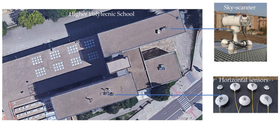
Figure 1. Experimental facility used in this study (Higher Polytechnic School, University of Burgos, Spain).

Various climatic parameters were recorded, including air temperature $\left(\mathrm{T}\right)$, relative humidity $\left(\mathrm{R}\mathrm{H}\right),$ wind speed $\left(\mathrm{W}\mathrm{S}\right),$ and direction. $\mathrm{G}\mathrm{H}\mathrm{I}$ and Diffuse Horizontal Irradiance ($\mathrm{D}\mathrm{H}\mathrm{I}$) were measured with Hulseflux pyranometers (model SR11) and Direct Normal Irradiance ($\mathrm{D}\mathrm{N}\mathrm{I}$) by means of a Hulseflux pyrheliometer (model DR01). A GEONICA-SEMS-3000 sun tracker equipped with a shading disc was employed for the measurement of $\mathrm{D}\mathrm{H}\mathrm{I}$. Additionally, the pyrheliometer was mounted on the sun tracker to measure $\mathrm{D}\mathrm{N}\mathrm{I}$. $\mathrm{G}\mathrm{H}\mathrm{U}\mathrm{V}\mathrm{E}$ values were obtained with a Kipp and Zonnen SUV-E radiometer. Sky luminance and radiance distributions, used to classify the sky condition, were determined with a sky-scanner EKO MS-321LR. The cloud cover $\left(\mathrm{C}\mathrm{C}\right)$ was calculated with a commercial all-sky camera (SONAD201D) that records every 1 s an RGB color image with 1158 × 1172 pixels of resolution. A complete description of the experimental facility and instruments can be found in previous works [42,43].

The collected $\mathrm{G}\mathrm{H}\mathrm{I}$, $\mathrm{G}\mathrm{H}\mathrm{U}\mathrm{V}\mathrm{E},$ $\mathrm{D}\mathrm{H}\mathrm{I}$, and $\mathrm{D}\mathrm{N}\mathrm{I}$ data underwent the quality control procedure recommended by the MESoR project [44]. For the $\mathrm{G}\mathrm{H}\mathrm{U}\mathrm{V}\mathrm{E}$ data, it was determined that $\mathrm{G}\mathrm{H}\mathrm{U}\mathrm{V}\mathrm{E}$ values should not exceed the corresponding extraterrestrial $\mathrm{U}\mathrm{V}\mathrm{E}\mathrm{R}$ on the horizontal plane ($\mathrm{U}\mathrm{V}\mathrm{E}{\mathrm{H}}_0$). The calculation of $\mathrm{U}\mathrm{V}\mathrm{E}{\mathrm{H}}_0$ involved applying a correction factor $\left({\mathrm{f}}_{\mathrm{c}}\right)$, which considered the estimated orbital eccentricity to the $\mathrm{U}\mathrm{V}\mathrm{E}\mathrm{R}$ solar constant ($\mathrm{U}\mathrm{V}{\mathrm{E}}_{\mathrm{s}\mathrm{c}}$) multiplied by the cosine of the solar zenith angle (${\mathsf{\theta }}_z$), as described in Equation (1).

$$\mathrm{U}\mathrm{V}\mathrm{E}{\mathrm{H}}_0={\mathrm{f}}_{\mathrm{c}}\cdot \mathrm{U}\mathrm{V}{\mathrm{E}}_{\mathrm{s}\mathrm{c}}\cdot \cos {\mathsf{\theta }}_{\mathrm{z}}$$

(1)

In the absence of a standardized value, $\mathrm{U}\mathrm{V}{\mathrm{E}}_{\mathrm{s}\mathrm{c}}$ was determined by integrating the product of the extraterrestrial solar spectrum [45] and the erythema spectral weighting function [14] over the wavelength range of 280 to 400 nm. This calculation yielded a value of 14.5 W·m⁻². Data points corresponding to solar elevation angles below $5°$ were excluded from the analysis to mitigate the cosine response issues inherent to the $\mathrm{G}\mathrm{H}\mathrm{I},$ and $\mathrm{G}\mathrm{H}\mathrm{U}\mathrm{V}\mathrm{E}$ measurement instruments.

A summary of the variables used in this study is shown in Table 2. Among these meteorological variables, the following were directly obtained from the experimental measurements: $\mathrm{G}\mathrm{H}\mathrm{I}$, $\mathrm{D}\mathrm{H}\mathrm{I}$, $\mathrm{D}\mathrm{N}\mathrm{I}$, $\mathrm{C}\mathrm{C}$, $\mathrm{R}\mathrm{H}$, $\mathrm{T},$ and $\mathrm{W}\mathrm{S}.$ ${\mathsf{\theta }}_z$, and $\mathsf{\psi }$ were calculated. The remaining variables, including diffuse fraction, $\mathrm{D}$ [46], ${\mathrm{k}}_{\mathrm{t}}$ [47], ${\mathrm{k}\mathrm{\text{'}}}_{\mathrm{d}}$, Perez´s brightness factor ($∆)$ [48], and Perez´s clearness index,$\mathsf{\epsilon }$ [48], were calculated using the equations described in Table 2.

Table 2. Variables measured and calculated in Burgos.

Variables.	Meteorological Variables	Expression
$\mathrm{G}\mathrm{H}\mathrm{I}$	Global Horizontal irradiance	measured
$\mathrm{D}\mathrm{H}\mathrm{I}$	Diffuse Horizontal irradiance	measured
$\mathrm{D}\mathrm{N}\mathrm{I}$	Direct Normal irradiance	measured
$\mathrm{C}\mathrm{C}$	Cloud cover	measured
$\mathrm{R}\mathrm{H}$	Relative Humidity	measured
$\mathrm{T}$	Air temperature	measured
$\mathrm{W}\mathrm{S}$	Wind speed	measured
ψ	Solar azimuth angle	calculated
${\mathsf{\theta }}_{\mathrm{z}}$	Solar zenith angle	calculated
$\mathrm{D}$	Diffuse fraction	$\mathrm{D}=\frac{\mathrm{D}\mathrm{H}\mathrm{I}}{\mathrm{G}\mathrm{H}\mathrm{I}}$
${\mathrm{k}}_{\mathrm{t}}$	Clearness index	${\mathrm{k}}_{\mathrm{t}}=\frac{\mathrm{G}\mathrm{H}\mathrm{I}}{{\mathrm{B}}_{\mathrm{s}\mathrm{c}}{\mathrm{f}}_{\mathrm{c}}\cos {\mathsf{\theta }}_{\mathrm{z}}}$
${\mathrm{k}´}_{\mathrm{d}}$	Diffuse to extraterrestrial irradiance	${\mathrm{k}}_{\mathrm{d}}=\frac{\mathrm{D}\mathrm{H}\mathrm{I}}{{\mathrm{B}}_{\mathrm{s}\mathrm{c}}}$
$∆$	Perez´s brightness factor	$∆=\frac{\mathrm{m}·\mathrm{D}\mathrm{H}\mathrm{I}}{{\mathrm{B}}_{\mathrm{s}\mathrm{c}}·{\mathrm{f}}_{\mathrm{c}}·\mathrm{c}\mathrm{o}\mathrm{s}{\mathsf{\theta }}_{\mathrm{z}}}$
$\mathsf{\epsilon }$	Perez´s clearness index	$\mathsf{\epsilon }=\frac{\frac{\mathrm{D}\mathrm{H}\mathrm{I}+\mathrm{D}\mathrm{N}\mathrm{I}}{\mathrm{D}\mathrm{H}\mathrm{I}}+\mathrm{k}{\left({\mathsf{\theta }}_{\mathrm{z}}\right)}^3}{1+\mathrm{k}{\left({\mathsf{\theta }}_{\mathrm{z}}\right)}^3}$

$B_{sc}$ is the solar constant ($1361.1 \mathrm{W}·{\mathrm{m}}^{-2}$ [49]). ${\mathrm{f}}_{\mathrm{c}}$ is the average value of the orbital eccentricity of the Earth. $k=1.04 (or 5.56·{10}^{-6}$ if ${\theta }_z$ is expressed in degrees).

The skies of the city of Burgos have been classified according to the $\mathrm{I}\mathrm{S}\mathrm{O}/\mathrm{C}\mathrm{I}\mathrm{E}$ standard [41], which considers the angular distribution of luminance in the sky measured by the sky scanner. The sky is classified into 15 different types, where types 1 to 5 are considered overcast skies, types 6 to 10 are categorized as intermediate skies, and sky types 11 to 15 are identified as clear skies. A complete description of the $\mathrm{I}\mathrm{S}\mathrm{O}/\mathrm{C}\mathrm{I}\mathrm{E}$ classification according to 15 types based on sky scanner measurements can be found in previous works [42,43].

Figure 2a illustrates the frequency of occurrence $\left(\mathrm{F}\mathrm{O}\mathrm{C}\right)$ of each $\mathrm{I}\mathrm{S}\mathrm{O}/\mathrm{C}\mathrm{I}\mathrm{E}$ standard sky type during the experimental campaign. Clear skies predominate in Burgos, with the most frequent sky type being classified as 13 (cloudless polluted with a wider solar corona). This sky type exceeds the 20% of all observed skies. When only the three main sky categories are considered, as shown in Figure 2b (overcast, intermediate, and clear), clear skies have the highest $\mathrm{F}\mathrm{O}\mathrm{C}$ (higher than 45%). This fact concurs with findings from previous studies conducted in Burgos [28].

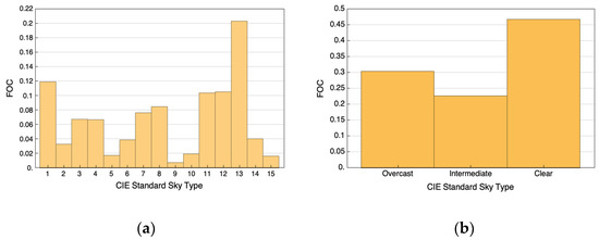
Figure 2. Frequency of occurrence $\left(\mathrm{F}\mathrm{O}\mathrm{C}\right)$ in Burgos (Spain) (a) of each $\mathrm{I}\mathrm{S}\mathrm{O}/\mathrm{C}\mathrm{I}\mathrm{E}$ standard sky type, and (b) for each $\mathrm{I}\mathrm{S}\mathrm{O}/\mathrm{C}\mathrm{I}\mathrm{E}$ sky type group.

The box and whisker plot of Figure 3 shows the distribution of the $\mathrm{G}\mathrm{H}\mathrm{U}\mathrm{V}\mathrm{E}/\mathrm{G}\mathrm{H}\mathrm{I}$ ratio based on 10 min data grouped by UTC hours, calculated from sunrise to sunset, using the complete database of the experimental campaign. The graph presents various statistical measures, including the mean value (gray crosses), the median (white lines inside the box), the interquartile range (the limits of the boxes), and both the maximum and minimum data values (the extreme whiskers), as well as the outlier values (black and gray circles). It can be observed that the hourly mean and median values of $\mathrm{G}\mathrm{H}\mathrm{U}\mathrm{V}\mathrm{E}/\mathrm{G}\mathrm{H}\mathrm{I}$ gradually increased until noon ($\mathrm{12:00} \mathrm{h}$) and then decreased until sunset. Higher dispersion of the values in the central hours of the day ($\mathrm{10:00} \mathrm{h}$ to $\mathrm{14:00} \mathrm{h}$) may be observed, as shown by the interquartile range (around $9 · {10}^{-3}\mathrm{\%}$). The maximum value ($4.2 · {10}^{-2}\%$) is reached at $\mathrm{12:00} \mathrm{h}$ $\mathrm{U}\mathrm{T}\mathrm{C}$.

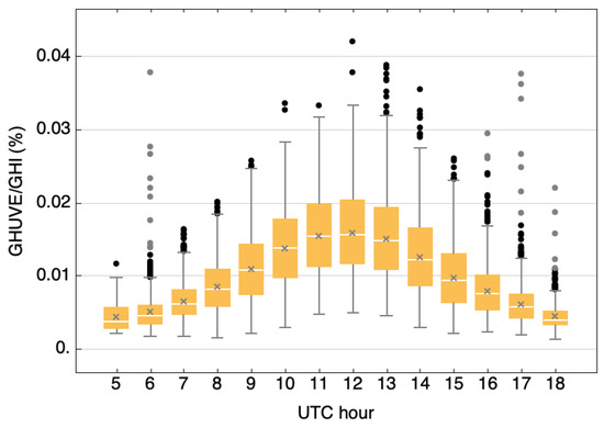
Figure 3. Box and whisker plot of the $\mathrm{G}\mathrm{H}\mathrm{U}\mathrm{V}\mathrm{E}/\mathrm{G}\mathrm{H}\mathrm{I}$ ratio based on 10 min data grouped by UTC hours. Gray crosses indicate the mean, and the white lines inside the box indicate the median. The limits of the boxes define the first, second, and third quartiles, whereas the extreme whiskers show the minimum and the maximum points. Black and gray circles represent outliers.

Figure 4 and Figure 5 show the statistical analysis of the 10 min data of the $\mathrm{G}\mathrm{H}\mathrm{U}\mathrm{V}\mathrm{E}/\mathrm{G}\mathrm{H}\mathrm{I}$ ratio grouped by month and season, respectively. Figure 4 reveals a gradual increase of $\mathrm{G}\mathrm{H}\mathrm{U}\mathrm{V}\mathrm{E}/\mathrm{G}\mathrm{H}\mathrm{I}$ until May, followed by practically constant values until August, and then a decrease for the rest of the year. The interquartile range fluctuated between $3 · {10}^{-3}\%$ and $1.2 · {10}^{-2}\mathrm{\%}$ and the standard deviation ranged between $3 · {10}^{-3}\%$ and $7 · {10}^{-3}\mathrm{\%}$. During the months from May to August, the ratio exhibited the greatest dispersion of the measurement campaign, with interquartile ranges around $1.1 · {10}^{-2}\mathrm{\%}$ and standard deviations around $6 · {10}^{-3}\mathrm{\%}$. The maximum value was recorded in July (4.2 $· {10}^{-2} ·$%), while the minimum was reached in April (1$·{10}^{-3}$%).

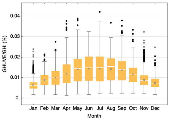
Figure 4. Box and whisker plot of the $\mathrm{G}\mathrm{H}\mathrm{U}\mathrm{V}\mathrm{E}/\mathrm{G}\mathrm{H}\mathrm{I}$ ratio based on 10 min data grouped by months.

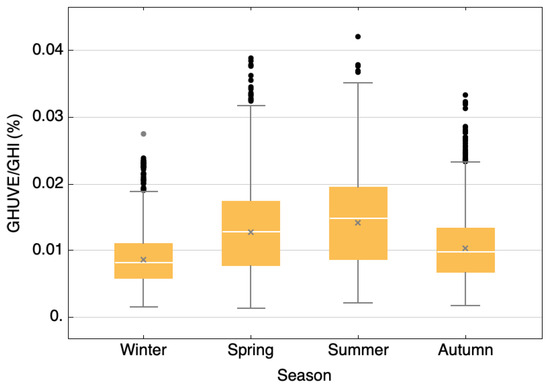
Figure 5. Box and whisker plot of the $\mathrm{G}\mathrm{H}\mathrm{U}\mathrm{V}\mathrm{E}/\mathrm{G}\mathrm{H}\mathrm{I}$ ratio based on 10 min data grouped by seasons.

Figure 5 shows the greatest dispersion of values for the summer months and the highest value of the $\mathrm{G}\mathrm{H}\mathrm{U}\mathrm{V}\mathrm{E}/\mathrm{G}\mathrm{H}\mathrm{I}$ ratio. Conversely, the dispersion of values in winter was relatively smaller. The interquartile ranges were $1.1 · {10}^{-2}\mathrm{\%}$ and 5 · ${10}^{-3}$% with standard deviations of $6 · {10}^{-3}\mathrm{\%}$ and 4 ∙${10}^{-3}$%, respectively.

Upon analyzing the $\mathrm{G}\mathrm{H}\mathrm{U}\mathrm{V}\mathrm{E}/\mathrm{G}\mathrm{H}\mathrm{I}$ ratio based on the 15 $\mathrm{I}\mathrm{S}\mathrm{O}/\mathrm{C}\mathrm{I}\mathrm{E}$ sky types (Figure 6), it is evident that sky type 15 exhibits the highest ratio value and the lowest data dispersion. Conversely, sky type 12 demonstrates the lowest ratio value, with an average level of data dispersion. Notably, both sky types belong to the category of clear skies.

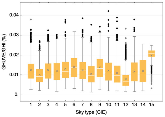
Figure 6. Box and whisker plot of the $\mathrm{G}\mathrm{H}\mathrm{U}\mathrm{V}\mathrm{E}/\mathrm{G}\mathrm{H}\mathrm{I}$ standard sky type (1 to 15).

Figure 7 shows that the variation between the mean $(1.1 · {10}^{-2}-1.2 · {10}^{-2}\mathrm{\%})$ and the dispersion (interquartile range: $8 · {10}^{-3}-9 · {10}^{-3}\mathrm{\%},$ standard deviation: $5 · {10}^{-3}-6 · {10}^{-3}\mathrm{\%})$ of the three main $\mathrm{I}\mathrm{S}\mathrm{O}/\mathrm{C}\mathrm{I}\mathrm{E}$ sky types is very similar.

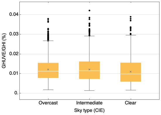
Figure 7. Box and whisker plot of the $\mathrm{G}\mathrm{H}\mathrm{U}\mathrm{V}\mathrm{E}/\mathrm{G}\mathrm{H}\mathrm{I}$ ratio based on 10 min data grouped by sky type group (overcast, intermediate, clear).

3. Methodology

3.1. Feature Selection

Feature selection $\left(\mathrm{F}\mathrm{S}\right)$ identifies the features that are related within a dataset, and it allows the elimination of irrelevant or unimportant features that contribute little or nothing to the definition of the target variable, providing more accurate models. This technique increases the performance of the developed model, improving its accuracy and reducing its complexity and overfitting, as well as its execution time.

In this study, to determine the most relevant meteorological variables for the estimation of $\mathrm{U}\mathrm{V}\mathrm{E}\mathrm{R}$, a selection of variables was performed based on the Pearson correlation coefficient $\left(\mathrm{r}\right),$ and the following rules: if $\mathrm{G}\mathrm{H}\mathrm{U}\mathrm{V}\mathrm{E}$ and one selected variable have a very weak relationship, the Pearson coefficient is 0; the relationship is very strong when r is close to 1 (direct correlation) or −1 (inverse correlation). To facilitate the assessment of correlation strength, the Thumb rule [50] established five r intervals for the correlation: direct $\left(1\ge \left|\mathrm{r}\left(\mathrm{G}\mathrm{H}\mathrm{U}\mathrm{V}\mathrm{E},\mathrm{v}\mathrm{a}\mathrm{r}\mathrm{i}\mathrm{a}\mathrm{b}\mathrm{l}\mathrm{e}\right)\right|\ge 0.9\right)$, strong $\left(0.9>\left|\mathrm{r}\left(\mathrm{G}\mathrm{H}\mathrm{U}\mathrm{V}\mathrm{E},\mathrm{v}\mathrm{a}\mathrm{r}\mathrm{i}\mathrm{a}\mathrm{b}\mathrm{l}\mathrm{e}\right)\right|\ge 0.7\right)$, moderate $\left(0.7>\left|\mathrm{r}\left(\mathrm{G}\mathrm{H}\mathrm{U}\mathrm{V}\mathrm{E},\mathrm{v}\mathrm{a}\mathrm{r}\mathrm{i}\mathrm{a}\mathrm{b}\mathrm{l}\mathrm{e}\right)\right|\ge 0.5\right)$, weak $\left(0.5>\left|\mathrm{r}\left(\mathrm{G}\mathrm{H}\mathrm{U}\mathrm{V}\mathrm{E},\mathrm{v}\mathrm{a}\mathrm{r}\mathrm{i}\mathrm{a}\mathrm{b}\mathrm{l}\mathrm{e}\right)\right|\ge 0.3\right)$, and negligible $\left(\left|\mathrm{r}\left(\mathrm{G}\mathrm{H}\mathrm{U}\mathrm{V}\mathrm{E},\mathrm{v}\mathrm{a}\mathrm{r}\mathrm{i}\mathrm{a}\mathrm{b}\mathrm{l}\mathrm{e}\right)\right|<0.3\right)$.

Table 3 shows the various intervals of Pearson’s coefficients calculated for the different meteorological variables. It can be observed that $\mathrm{G}\mathrm{H}\mathrm{I}$ exhibits a very strong and direct influence on $\mathrm{G}\mathrm{H}\mathrm{U}\mathrm{V}\mathrm{E}$ for all-skies, overcast, and clear skies, while for intermediate skies, $\mathrm{G}\mathrm{H}\mathrm{I}$ is strongly correlated. In clear skies, ${\theta }_z$ is also very strong and is inversely correlated with $\mathrm{G}\mathrm{H}\mathrm{U}\mathrm{V}\mathrm{E}$, while for all-skies, overcast, and intermediate skies, this variable is strongly correlated. Likewise, in the case of all-sky types, ${\mathrm{k}}_{\mathrm{t}}$, $\mathrm{D}$, $\mathsf{\epsilon }$, $\mathrm{R}\mathrm{H}$, $\mathrm{D}\mathrm{N}\mathrm{I}$, and $\mathrm{T}$ have a moderate relationship with $\mathrm{G}\mathrm{H}\mathrm{U}\mathrm{V}\mathrm{E}$. When analyzing overcast skies, a direct and strong relationship with ${\mathrm{k}´}_{\mathrm{d}}$ and $\mathrm{D}\mathrm{H}\mathrm{I}$ is observed, and a moderate relation with ${\mathrm{k}}_{\mathrm{t}}$, $\mathrm{D}$, $∆$, $\mathrm{D}\mathrm{N}\mathrm{I}$. For intermediate skies, the relation between $\mathrm{G}\mathrm{H}\mathrm{U}\mathrm{V}\mathrm{E}$ and ${\mathrm{k}}_{\mathrm{t}}$, ${\mathrm{k}´}_{\mathrm{d}}$, $\mathrm{D}$, $\mathrm{D}\mathrm{H}\mathrm{I},\mathrm{a}\mathrm{n}\mathrm{d} \mathrm{D}\mathrm{N}\mathrm{I}$ is moderate. $\mathrm{W}\mathrm{S}$, ψ, and $\mathrm{C}\mathrm{C}$ present a negligible relation with $\mathrm{G}\mathrm{H}\mathrm{U}\mathrm{V}\mathrm{E}$, so these meteorological variables were discarded as inputs for modeling $\mathrm{G}\mathrm{H}\mathrm{U}\mathrm{V}\mathrm{E}$. These findings agree with the literature, which identifies $\mathrm{G}\mathrm{H}\mathrm{I}$ and ${\mathsf{\theta }}_z$ as the two variables that strongly influence $\mathrm{G}\mathrm{H}\mathrm{U}\mathrm{V}\mathrm{E}$ measurements [18,19,31]. Meteorological variables whose relationship with $\mathrm{G}\mathrm{H}\mathrm{U}\mathrm{V}\mathrm{E}$ is moderate, strong, or very strong $\left(\mathrm{r}\ge 0.5\right)$ have been selected.

Table 3. Pearson’s coefficients were calculated for the different variables.

$\left|\mathbf{r}\left(\mathbf{G}\mathbf{H}\mathbf{U}\mathbf{V}\mathbf{E},\mathbf{V}\mathbf{a}\mathbf{r}\mathbf{i}\mathbf{a}\mathbf{b}\mathbf{l}\mathbf{e}\right)\right|.$
CIE Sky Type	[1–0.9]	(0.9–0.7]	(0.7–0.5]	(0.5–0.3]	(0.3,0]
All-sky	$\mathrm{G}\mathrm{H}\mathrm{I}$	${\mathsf{\theta }}_{\mathrm{z}}$	${\mathrm{k}}_{\mathrm{t}}$$, \mathrm{D}$$, \mathsf{\epsilon }$$, \mathrm{R}\mathrm{H}$$, \mathrm{D}\mathrm{N}\mathrm{I}$$, \mathrm{T}$	${\mathrm{k}´}_{\mathrm{d}}$$, \mathrm{D}\mathrm{H}\mathrm{I}$	$∆$$, \mathrm{W}\mathrm{S}$$, \mathsf{\psi }, \mathrm{C}\mathrm{C}$
Overcast	$\mathrm{G}\mathrm{H}\mathrm{I}$	${\mathsf{\theta }}_{\mathrm{z}},{\mathrm{k}´}_{\mathrm{d}}$$, \mathrm{D}\mathrm{H}\mathrm{I}$	${\mathrm{k}}_{\mathrm{t}}$$, \mathrm{D}$$, \mathrm{D}\mathrm{N}\mathrm{I},∆$,	$\mathsf{\epsilon }$$, \mathrm{R}\mathrm{H}$$, \mathrm{T}$	$\mathrm{W}\mathrm{S}$$, \mathsf{\psi }, \mathrm{C}\mathrm{C}$
Intermediate	-	$\mathrm{G}\mathrm{H}\mathrm{I}$$, {\mathsf{\theta }}_{\mathrm{z}}$	${\mathrm{k}}_{\mathrm{t}}$$, {\mathrm{k}´}_{\mathrm{d}}$$, \mathrm{D}$$, \mathrm{D}\mathrm{H}\mathrm{I}$$, \mathrm{D}\mathrm{N}\mathrm{I}$	$\mathsf{\epsilon }$$, \mathrm{R}\mathrm{H}$$, \mathrm{T}$	$∆$$, \mathrm{W}\mathrm{S}$$, \mathsf{\psi }, \mathrm{C}\mathrm{C}$
Clear	$\mathrm{G}\mathrm{H}\mathrm{I}$$, {\mathsf{\theta }}_{\mathrm{z}}$	-	$\mathrm{T}$	${\mathrm{k}}_{\mathrm{t}}$$, {\mathrm{k}´}_{\mathrm{d}}$$, \mathrm{D}$$, \mathsf{\epsilon }$$, \mathrm{R}\mathrm{H}$$, \mathrm{D}\mathrm{N}\mathrm{I}$	$∆,\mathrm{D}\mathrm{H}\mathrm{I},\mathrm{W}\mathrm{S}$$, \mathsf{\psi }, \mathrm{C}\mathrm{C}$

3.2. Multilinear Regression Model

Meteorological variables selected in Section 3.1 were used as input variables for both $\mathrm{M}\mathrm{L}\mathrm{R}$ and $\mathrm{A}\mathrm{N}\mathrm{N}$ models. Four $\mathrm{M}\mathrm{L}\mathrm{R}$ models were developed: one for all skies and three additional specific models for the clear, intermediate, and overcast sky types. To develop the $\mathrm{M}\mathrm{L}\mathrm{R}$ models, the data were divided into two groups: the first group, comprising $85\mathrm{\%}$ of the data, was used for model fitting, and the remaining $15\mathrm{\%}$ of the data was used for model validation. Conventional statistics were employed to evaluate the adequacy of fit for each model: coefficient of determination (${\mathrm{R}}^2$), normalized root mean square error ($\mathrm{n}\mathrm{R}\mathrm{M}\mathrm{S}\mathrm{E}$) and normalized mean bias error ($\mathrm{n}\mathrm{M}\mathrm{B}\mathrm{E}$), calculated by Equations (2)–(4), respectively.

$${\mathrm{R}}^2=\frac{{\sum }_{\mathrm{i}=1}^{\mathrm{n}}({\mathrm{G}\mathrm{H}\mathrm{U}\mathrm{V}\mathrm{E}}_{\mathrm{m}\mathrm{o}\mathrm{d}}-{\overline{\mathrm{G}\mathrm{H}\mathrm{U}\mathrm{V}\mathrm{E}}}_{\mathrm{m}\mathrm{o}\mathrm{d}})·({\mathrm{G}\mathrm{H}\mathrm{U}\mathrm{V}\mathrm{E}}_{\mathrm{e}\mathrm{x}\mathrm{p}}-{\overline{\mathrm{G}\mathrm{H}\mathrm{U}\mathrm{V}\mathrm{E}}}_{\mathrm{e}\mathrm{x}\mathrm{p}})}{\sqrt{{\sum }_{\mathrm{i}=1}^{\mathrm{n}}{[\left({\mathrm{G}\mathrm{H}\mathrm{U}\mathrm{V}\mathrm{E}}_{\mathrm{m}\mathrm{o}\mathrm{d}}-\overline{{\mathrm{G}\mathrm{H}\mathrm{U}\mathrm{V}\mathrm{E}}_{\mathrm{m}\mathrm{o}\mathrm{d}}}\right)}^2{·\left({\mathrm{G}\mathrm{H}\mathrm{U}\mathrm{V}\mathrm{E}}_{\mathrm{e}\mathrm{x}\mathrm{p}}-\overline{{\mathrm{G}\mathrm{H}\mathrm{U}\mathrm{V}\mathrm{E}}_{\mathrm{e}\mathrm{x}\mathrm{p}}}\right)}^2]}}$$

(2)

$$\mathrm{n}\mathrm{R}\mathrm{M}\mathrm{S}\mathrm{E}=\frac{1}{{\overline{\mathrm{G}\mathrm{H}\mathrm{U}\mathrm{V}\mathrm{E}}}_{\mathrm{e}\mathrm{x}\mathrm{p}}}\sqrt{\frac{\sum _{\mathrm{i}=1}^{\mathrm{n}}{\left({\mathrm{G}\mathrm{H}\mathrm{U}\mathrm{V}\mathrm{E}}_{\mathrm{m}\mathrm{o}\mathrm{d}}-{\mathrm{G}\mathrm{H}\mathrm{U}\mathrm{V}\mathrm{E}}_{\mathrm{e}\mathrm{x}\mathrm{p}}\right)}^2}{\mathrm{n}}}100\left(\mathrm{\%}\right)$$

(3)

$$\mathrm{n}\mathrm{M}\mathrm{B}\mathrm{E}=\frac{1}{{\overline{\mathrm{G}\mathrm{H}\mathrm{U}\mathrm{V}\mathrm{E}}}_{\mathrm{e}\mathrm{x}\mathrm{p}}}\frac{\sum _{\mathrm{i}=1}^{\mathrm{n}}\left({\mathrm{G}\mathrm{H}\mathrm{U}\mathrm{V}\mathrm{E}}_{\mathrm{m}\mathrm{o}\mathrm{d}}-{\mathrm{G}\mathrm{H}\mathrm{U}\mathrm{V}\mathrm{E}}_{\mathrm{e}\mathrm{x}\mathrm{p}}\right)}{\mathrm{n}}100\left(\mathrm{\%}\right)$$

(4)

where $\mathrm{n}$ represents the number of experimental data points used for model fitting and testing in each case; ${\mathrm{G}\mathrm{H}\mathrm{U}\mathrm{V}\mathrm{E}}_{\mathrm{e}\mathrm{x}\mathrm{p}}$ is the experimental value of $\mathrm{G}\mathrm{H}\mathrm{U}\mathrm{V}\mathrm{E}$, and ${\mathrm{G}\mathrm{H}\mathrm{U}\mathrm{V}\mathrm{E}}_{\mathrm{m}\mathrm{o}\mathrm{d}}$ is the modeled $\mathrm{G}\mathrm{H}\mathrm{U}\mathrm{V}\mathrm{E}$ value.

The mathematical expressions of the four regression models and the goodness of fit of each one are shown in Table 4. The model’s fitting results presented a high determination coefficient with the experimental data (${\mathrm{R}}^2>0.92$); however, the $\mathrm{n}\mathrm{R}\mathrm{M}\mathrm{S}\mathrm{E}$ values obtained through multilinear regressions exceeded 20% in all cases.

Table 4. Multilinear regression (MLR) models of $\mathrm{G}\mathrm{H}\mathrm{U}\mathrm{V}\mathrm{E}$ and goodness of fit (based on 85% of data).

Sky Types	$\mathbf{M}\mathbf{L}\mathbf{R}$ Model	${\mathbf{R}}^2$	$\mathbf{n}\mathbf{R}\mathbf{S}\mathbf{M}\mathbf{E}$(%)	nMBE (%)
All skies	$\begin{array}{c}\mathrm{G}\mathrm{H}\mathrm{U}\mathrm{V}\mathrm{E}=1.90·{10}^{-2}+2.35·{10}^{-4}\mathrm{G}\mathrm{H}\mathrm{I}-1.74·{10}^{-2}{\mathsf{\theta }}_{\mathrm{z}}-9.85·\\ {10}^{-2}{\mathrm{k}}_{\mathrm{t}}+7.44·{10}^{-4}\mathrm{T}\end{array}$	$0.937$	$25.60$	$-2.05·{10}^{-1212}$
Overcast	$\begin{array}{c}\mathrm{G}\mathrm{H}\mathrm{U}\mathrm{V}\mathrm{E}=2.98·{10}^{-2}+1.61·{10}^{-4}\mathrm{G}\mathrm{H}\mathrm{I}-2.71·{10}^{-2}{\mathsf{\theta }}_{\mathrm{z}}\\ +1.30{\mathrm{k}´}_{\mathrm{d}}-9.89·{10}^{-4}\mathrm{D}\mathrm{H}\mathrm{I}\end{array}$	$0.926$	$29.80$	$6.92·{10}^{-13}$
Intermediate	$\begin{array}{c}\mathrm{G}\mathrm{H}\mathrm{U}\mathrm{V}\mathrm{E}=8.54·{10}^{-2}+2.59·{10}^{-4}\mathrm{G}\mathrm{H}\mathrm{I}-6.98·{10}^{-2}{\mathsf{\theta }}_{\mathrm{z}}-1.80·\\ {10}^{-4}\mathrm{D}\mathrm{H}\mathrm{I}-9.91·{10}^{-5}\mathrm{D}\mathrm{N}\mathrm{I}\end{array}$	$0.934$	$22.49$	$3.23·{10}^{-12}$
Clear	$\begin{array}{c}\mathrm{G}\mathrm{H}\mathrm{U}\mathrm{V}\mathrm{E}=1.75 · {10}^{-1}+5.84 · {10}^{-5}\mathrm{G}\mathrm{H}\mathrm{I}-1.52 · {10}^{-1}{\mathsf{\theta }}_{\mathrm{z}}+6.89 · \\ {10}^{-4}\mathrm{T}\end{array}$	$0.940$	$21.10$	$9.87·{10}^{-13}$

3.3. Artificial Neural Network Model

In this work, $\mathrm{A}\mathrm{N}\mathrm{N}\mathrm{s}$ were used to estimate $\mathrm{G}\mathrm{H}\mathrm{U}\mathrm{V}\mathrm{E}$ through the Levenberg–Marquardt Back-Propagation ($\mathrm{L}\mathrm{M}\mathrm{B}\mathrm{P}$) algorithm. The $\mathrm{A}\mathrm{N}\mathrm{N}$ architecture adopted for this purpose consists of a single hidden layer and a single output, as outlined in a previous publication [28,29]. In the input layer, each neuron is a meteorological variable. Determining the optimal number of neurons in the hidden layer is currently unknown, but it is acknowledged that this number should not exceed the number of neurons in the preceding layer [51]. Therefore, if the input layer has only one variable and thus a single neuron, the hidden layer can have only one neuron. If the input layer has two meteorological variables, the hidden layer can have either one or two neurons. Similarly, if the input has three variables and, therefore, three neurons, the hidden layer can have three, two, or one neuron/s, and this trend continues for additional variables in the input layer. The iterative process and the fitting are explained elsewhere [28].

Four $\mathrm{A}\mathrm{N}\mathrm{N}$ models were generated and tested in this work, one for all skies and three for each sky type (clear, intermediate, and overcast), considering the selected meteorological variables shown in Table 3. Table 5 shows the goodness of fit for each $\mathrm{A}\mathrm{N}\mathrm{N}$ model according to the described statistics. It can be observed that in four cases, a good determination coefficient was obtained, ${\mathrm{R}}^2>0.95.$ The $\mathrm{n}\mathrm{R}\mathrm{S}\mathrm{M}\mathrm{E}$ obtained varied between $11.9\mathrm{\%}$ and $21.3\mathrm{\%}$. The best results were obtained for clear skies (${\mathrm{R}}^2>0.98$ and $\mathrm{n}\mathrm{R}\mathrm{M}\mathrm{S}\mathrm{E}<12\mathrm{\%}$).

Table 5. Goodness of fit of the $\mathrm{ANN}$ models (based on 85% of data).

Sky Condition	${\mathrm{R}}^2$	$\mathrm{nRMSE} (\%)$	$\mathrm{nMBE} (\%)$
All skies (MLR1)	$0.988$	$14.36$	$6.69 · {10}^{-2}$
Overcast	$0.962$	$21.32$	$6.69 · {10}^{-2}$
Intermediate	$0.955$	$18.68$	$9.09 · {10}^{-2}$
Clear	$0.981$	$11.92$	$7.59 · {10}^{-3}$

4. Results and Discussion

The remaining $15\mathrm{\%}$ of the data, not used previously for generating the MLR and $\mathrm{A}\mathrm{N}\mathrm{N}$ models, were used as a validation set for both $\mathrm{M}\mathrm{L}\mathrm{R}$ and $\mathrm{A}\mathrm{N}\mathrm{N}$ models. The results are shown in Table 6, with $\mathrm{M}\mathrm{L}\mathrm{R}$ outcomes on the left and $\mathrm{A}\mathrm{N}\mathrm{N}$ results on the right. The best results were obtained for clear skies (${\mathrm{R}}^2>0.97,$ and $\mathrm{n}\mathrm{R}\mathrm{M}\mathrm{S}\mathrm{E}<12.4\mathrm{\%}$). Both nRMSE and nMBE values obtained through multilinear regressions exceeded 20% in all cases, results close to those obtained by other authors [2] who performed models using second-degree polynomials, obtaining nRMSE values between 20% and 54%. Previous works modeled hourly [31] and daily [34,35,36,37] $\mathrm{G}\mathrm{H}\mathrm{U}\mathrm{V}\mathrm{E}$ values through ANN obtaining $\mathrm{n}\mathrm{R}\mathrm{M}\mathrm{S}\mathrm{E}$ ranging from 14 and 21%. Considerable improvement in performances occurred when the highly influential parameter $\mathrm{T}\mathrm{O}\mathrm{C}$ was introduced as ANN input.

Table 6. Goodness of fit of $\mathrm{M}\mathrm{L}\mathrm{R}$ and $\mathrm{A}\mathrm{N}\mathrm{N}$ models (based on 15% of data).

Sky Condition	${\mathbf{R}}^2$	$\mathbf{n}\mathbf{R}\mathbf{S}\mathbf{M}\mathbf{E}$ (%)	$\mathbf{n}\mathbf{M}\mathbf{B}\mathbf{E}$ (%)	Sky Condition	${\mathbf{R}}^2$	$\mathbf{n}\mathbf{R}\mathbf{S}\mathbf{M}\mathbf{E}$ (%)	$\mathbf{n}\mathbf{M}\mathbf{B}\mathbf{E}$ (%)
All skies (MLR1)	$0.938$	$25.21$	$1.41 · {10}^{-1 }$	All skies (ANN1)	$0.979$	$14.63$	$1.55 · {10}^{-1 }$
Overcast (MLR2)	$0.930$	$29.65$	$6.28 · {10}^{-1 }$	Overcast (ANN2)	$0.965$	$21.06$	$6.58 · {10}^{-1 }$
Intermediate (MLR3)	$0.923$	$23.57$	$-5.75 · {10}^{-1 }$	Intermediate (ANN3)	$0.953$	$19.20$	$3.38 · {10}^{-1 }$
Clear (MLR4)	$0.942$	$20.57$	$-2.10 · {10}^{-1 }$	Clear (ANN4)	$0.979$	$12.35$	$4.31 · {10}^{-1 }$

Table 6 comparison revealed that $\mathrm{A}\mathrm{N}\mathrm{N}$ models performed better than $\mathrm{M}\mathrm{L}\mathrm{R}$ models. For all skies and clear skies, the $\mathrm{n}\mathrm{R}\mathrm{M}\mathrm{S}\mathrm{E}$ value improved significantly, decreasing over 40% with respect to the $\mathrm{M}\mathrm{L}\mathrm{R}$ models. The $\mathrm{n}\mathrm{M}\mathrm{B}\mathrm{E}$ value was overestimated for intermediate and clear skies.

Figure 8 and Figure 9 compare the modeled $\mathrm{G}\mathrm{H}\mathrm{U}\mathrm{V}\mathrm{E}$ values from derived $\mathrm{M}\mathrm{L}\mathrm{R}$ models and ANN models, respectively, and the corresponding experimental $\mathrm{G}\mathrm{H}\mathrm{U}\mathrm{V}\mathrm{E}$ measurements obtained from the Burgos meteorological station using the referred validation data set. A good determination coefficient was obtained (${\mathrm{R}}^2>0.92$, MRL models, ${\mathrm{R}}^2>0.95$ ANN models) both for all skies, overcast, intermediate, and clear sky conditions.

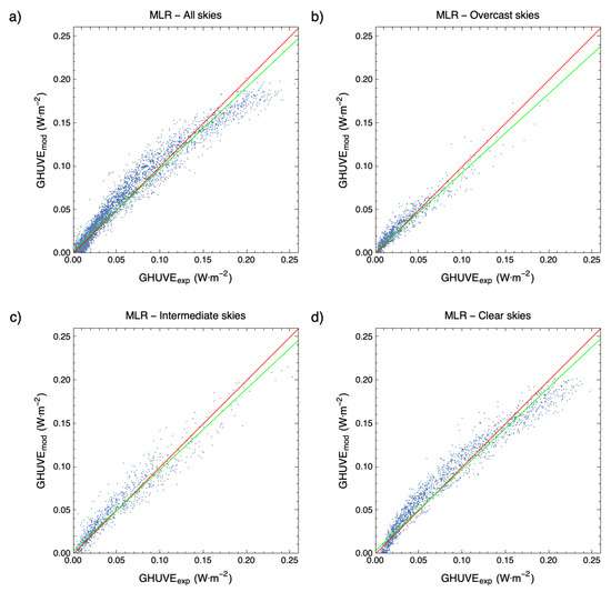
Figure 8. Comparison between calculated (${\mathrm{G}\mathrm{H}\mathrm{U}\mathrm{V}\mathrm{E}}_{\mathrm{m}\mathrm{o}\mathrm{d}}$) from MLR models and experimental ${\mathrm{G}\mathrm{H}\mathrm{U}\mathrm{V}\mathrm{E}}_{\mathrm{e}\mathrm{x}\mathrm{p}}$ data under different sky conditions: (a) all skies, (b) overcast, (c) partial, and (d) clear skies. The green line represents the fitting line; the red line represents the x = y line.

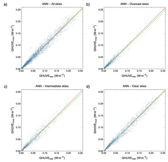
Figure 9. Comparison between calculated (${\mathrm{G}\mathrm{H}\mathrm{U}\mathrm{V}\mathrm{E}}_{\mathrm{m}\mathrm{o}\mathrm{d}}$) from ANN models and experimental ${\mathrm{G}\mathrm{H}\mathrm{U}\mathrm{V}\mathrm{E}}_{\mathrm{e}\mathrm{x}\mathrm{p}}$ data under different sky conditions: (a) all skies, (b) overcast, (c) partial, and (d) clear skies. The green line represents the fitting line; the red line represents the x = y line.

To improve the previous results, a new approach was introduced to optimize the number of variables for minimizing $\mathrm{n}\mathrm{R}\mathrm{M}\mathrm{S}\mathrm{E}$ using $\mathrm{A}\mathrm{N}\mathrm{N}$ models for all-sky conditions. The number of neurons in the hidden layer can be adjusted accordingly to accommodate the complexity and dimensionality of the input data, from one neuron to the number of input variables of the ANN.

The two variables identified as strongly correlated to $\mathrm{G}\mathrm{H}\mathrm{U}\mathrm{V}\mathrm{E}$ based on Pearson’s coefficient, as shown in Table 3, $\mathrm{G}\mathrm{H}\mathrm{I}$ and ${\mathsf{\theta }}_{\mathrm{z}}$, were used as reference in this study. The $\mathrm{A}\mathrm{N}\mathrm{N}$ with two neurons in the hidden layer, with $\mathrm{G}\mathrm{H}\mathrm{I}$ and ${\mathsf{\theta }}_{\mathrm{z}}$ as input variables presented $\mathrm{n}\mathrm{R}\mathrm{M}\mathrm{S}\mathrm{E}$ of $17.02\mathrm{\%}$, as shown in Table 7. By retaining $\mathrm{G}\mathrm{H}\mathrm{I}$ and ${\mathsf{\theta }}_{\mathrm{z}}$ as input variables, new $\mathrm{A}\mathrm{N}\mathrm{N}$ models were generated, increasing one by one the number of variables included in Table 2 and, consequently, the number of neurons in the hidden layer, from one neuron to as many neurons as the number of variables in each case.

Table 7. $\mathrm{n}\mathrm{R}\mathrm{M}\mathrm{S}\mathrm{E}$ for $\mathrm{A}\mathrm{N}\mathrm{N}$ model $\left(\mathrm{G}\mathrm{H}\mathrm{I}{,\mathsf{\theta }}_{\mathrm{z}}\right)$ calculated with one and two neurons.

All-Skies	$\mathbf{n}\mathbf{R}\mathbf{M}\mathbf{S}\mathbf{E}$(%)
	One neuron	Two neurons
$\mathrm{G}\mathrm{H}\mathrm{I},{\mathsf{\theta }}_{\mathrm{z}}$	$18.65$	$17.02$

Table 8 shows the percentage of $\mathrm{G}\mathrm{H}\mathrm{U}\mathrm{V}\mathrm{E}$ $\mathrm{A}\mathrm{N}\mathrm{N}$ models resulting from combinations of input variables out of the total of possible combinations for each case, whose $\mathrm{n}\mathrm{R}\mathrm{M}\mathrm{S}\mathrm{E}$ was below $15\mathrm{\%}$. For the combination of five variables, with two to five neurons in the hidden layer, $\mathrm{n}\mathrm{R}\mathrm{M}\mathrm{S}\mathrm{E}<15\mathrm{\%}$ was obtained for 5%, 25%, 28%, and $30\mathrm{\%}$ of the generated $\mathrm{A}\mathrm{N}\mathrm{N}\mathrm{s}$, respectively. For the combination of six variables, from two neurons to six neurons, $\mathrm{n}\mathrm{R}\mathrm{M}\mathrm{S}\mathrm{E}<15\mathrm{\%}$ was obtained for the range $22-57\mathrm{\%}$ of the generated $\mathrm{A}\mathrm{N}\mathrm{N}$ models.

Table 8. Percentage of generated $\mathrm{G}\mathrm{H}\mathrm{U}\mathrm{V}\mathrm{E}$ $\mathrm{A}\mathrm{N}\mathrm{N}$ models, according to number of input variables and number of neurons, with $\mathrm{n}\mathrm{R}\mathrm{S}\mathrm{M}\mathrm{E}<15\mathrm{\%}.$.

		Number of Input Variables
Number of neurons in the hidden layer		3	4	5	6
	1	0	0	0	0
	2	0	2	5	22
	3	8	14	25	27
	4		18	28	41
	5			30	48
	6				57

Table 9 shows the combinations of five and six input variables ranging from two to six neurons in the $\mathrm{A}\mathrm{N}\mathrm{N}$ hidden layer, which estimated the lowest $\mathrm{n}\mathrm{R}\mathrm{M}\mathrm{S}\mathrm{E}$. Among the various $\mathrm{A}\mathrm{N}\mathrm{N}$ models considered, despite its slightly higher error, Model 2 was considered the optimal model due to the use as input data variables that are commonly measured at ground radiometric stations. The practical advantage of this model lies in the accessibility and availability of $\mathrm{G}\mathrm{H}\mathrm{I}$, ${\mathsf{\theta }}_{\mathrm{z}}$, $\mathrm{T}$, ${\mathrm{k}}_{\mathrm{t}}$, and $\mathsf{\psi }$ data, making it easier to implement in real-world scenarios without the need for additional specialized measurements. In contrast, the other models are based on meteorological variables that are not frequently recorded at meteorological stations. $\mathrm{A}\mathrm{N}\mathrm{N}$ Models 3, 7, 8, and 9 depend on $\mathrm{C}\mathrm{C}$, which requires the use of a sky camera. Models 1, 4, 5, and 6 rely on $\mathrm{D}\mathrm{H}\mathrm{I}$, thus requiring the use of a pyrheliometer and a solar tracker, elements of high cost and complex maintenance, and, therefore, scarce in meteorological ground facilities.

Table 9. Performance $(\mathrm{n}\mathrm{R}\mathrm{S}\mathrm{M}\mathrm{E}$ (%)) of $\mathrm{A}\mathrm{N}\mathrm{N}$ models of $\mathrm{G}\mathrm{H}\mathrm{U}\mathrm{V}\mathrm{E},$ generated from combinations of five and six experimental meteorological variables and from two to six neurons in the hidden layer.

$\mathbf{A}\mathbf{N}\mathbf{N}$	Number of Variables/Neurons in the Hidden Layer	Meteorological Variables	$\mathbf{R}\mathbf{S}\mathbf{M}\mathbf{E}\left(\mathbf{\%}\right)$
Model 1	5/2	$\mathrm{G}\mathrm{H}\mathrm{I},{\mathsf{\theta }}_{\mathrm{z}},\mathsf{\epsilon },\mathrm{T},{\mathrm{k}}_{\mathrm{t}}$	$14.49$
Model 2	5/3	$\mathrm{G}\mathrm{H}\mathrm{I},{\mathsf{\theta }}_{\mathrm{z}},\mathrm{T},{\mathrm{k}}_{\mathrm{t}},\mathsf{\psi }$	$14.16$
Model 3	5/4	$\mathrm{G}\mathrm{H}\mathrm{I},{\mathsf{\theta }}_{\mathrm{z}},\mathrm{T}, \mathrm{C}\mathrm{C},\mathsf{\psi }$	$13.34$
Model 4	5/5	$\mathrm{G}\mathrm{H}\mathrm{I},{\mathsf{\theta }}_{\mathrm{z}}, \mathrm{T}, ∆,\mathsf{\psi }$	$13.01$
Model 5	6/2	$\mathrm{G}\mathrm{H}\mathrm{I},{\mathsf{\theta }}_{\mathrm{z}},{\mathrm{k}}_{\mathrm{t}},\mathsf{\epsilon },\mathrm{T},\mathrm{R}\mathrm{H}$	$14.11$
Model 6	6/3	$\mathrm{G}\mathrm{H}\mathrm{I},{\mathsf{\theta }}_{\mathrm{z}},\mathrm{D}\mathrm{H}\mathrm{I},\mathrm{T},\mathrm{R}\mathrm{H},\mathsf{\psi }$	$13.59$
Model 7	6/4	$\mathrm{G}\mathrm{H}\mathrm{I},{\mathsf{\theta }}_{\mathrm{z}},\mathrm{T},\mathrm{R}\mathrm{H},\mathrm{C}\mathrm{C},\mathsf{\psi }$	$12.94$
Model 8	6/5	$\mathrm{G}\mathrm{H}\mathrm{I},{\mathsf{\theta }}_{\mathrm{z}},\mathrm{T},\mathrm{R}\mathrm{H},\mathrm{C}\mathrm{C},\mathsf{\psi }$	$12.53$
Model 9	6/6	$\mathrm{G}\mathrm{H}\mathrm{I},{\mathsf{\theta }}_{\mathrm{z}},{\mathrm{k}}_{\mathrm{t}},\mathrm{T},\mathrm{C}\mathrm{C},\mathsf{\psi }$	$12.16$

5. Conclusions

This study was based on the experimental data recorded and analyzed at 10 min intervals between September 2020 and June 2022 in Burgos (Spain). The $\mathrm{G}\mathrm{H}\mathrm{U}\mathrm{V}\mathrm{E}/\mathrm{G}\mathrm{H}\mathrm{I}$ ratio was analyzed at different time intervals as a function of the sky type classified according to the $\mathrm{I}\mathrm{S}\mathrm{O}/\mathrm{C}\mathrm{I}\mathrm{E}$ standard. The analysis of the $\mathrm{G}\mathrm{H}\mathrm{U}\mathrm{V}\mathrm{E}/\mathrm{G}\mathrm{H}\mathrm{I}$ ratio yielded a gradual increase from dawn to noon (12:00 h) and a subsequent decrease until sunset. A greater dispersion of values was observed in the central hours of the day (10:00 a.m. to 2:00 p.m.). The relationship showed higher values with a higher dispersion for the months from May until August and lower values in December and January. The value of the ratio and the data dispersion into the three categories (overcast, intermediate, and clear skies) was very similar.

Different models were analyzed to determine $\mathrm{G}\mathrm{H}\mathrm{U}\mathrm{V}\mathrm{E}$ based on meteorological and radiative variables collected in Burgos, using multilinear regression models ($\mathrm{M}\mathrm{L}\mathrm{R}$) and artificial neural network ($\mathrm{A}\mathrm{N}\mathrm{N}$) for all skies, overcast, intermediate, and clear skies. The use of variables from databases or satellite observation was not considered to guarantee, as far as possible, the applicability of locally obtained models in other locations using data from ground meteorological facilities.

The $\mathrm{M}\mathrm{L}\mathrm{R}$ model fitting results presented high determination coefficients with the experimental data (${\mathrm{R}}^2>0.92$) for all skies, overcast, intermediate, and clear skies. However, the $\mathrm{n}\mathrm{R}\mathrm{M}\mathrm{S}\mathrm{E}$ value was elevated, exceeding 20% in the four cases. Since the $\mathrm{M}\mathrm{L}\mathrm{R}$ models did not perform as expected, $\mathrm{G}\mathrm{H}\mathrm{U}\mathrm{V}\mathrm{E}$ was modeled by $\mathrm{A}\mathrm{N}\mathrm{N}$ models, considering the variables used for $\mathrm{M}\mathrm{L}\mathrm{R}$ modeling for each sky type. In all four cases, a good determination coefficient was obtained, ${\mathrm{R}}^2>0.95$. The $\mathrm{n}\mathrm{R}\mathrm{S}\mathrm{M}\mathrm{E}$ obtained varied between 12 and 21%. The best results were obtained for clear skies (${\mathrm{R}}^2>0.97$ and $\mathrm{n}\mathrm{R}\mathrm{M}\mathrm{S}\mathrm{E}<12.4\mathrm{\%}$).

For all skies, the optimal number of variables was evaluated to achieve an $\mathrm{n}\mathrm{R}\mathrm{M}\mathrm{S}\mathrm{E}$ of less than 15% by means of $\mathrm{A}\mathrm{N}\mathrm{N}$ models. Through the derivation and analysis of multiple models, it was determined that the adequate choice was the model encompassing $\mathrm{G}\mathrm{H}\mathrm{I},{\mathsf{\theta }}_{\mathrm{z}},\mathrm{T},{\mathrm{k}}_{\mathrm{t}},\mathsf{\psi }$, due to its high performance and the availability of the required inputs from most ground meteorological facilities.

Future research endeavors should incorporate the deeply impactful total ozone column ($\mathrm{T}\mathrm{O}\mathrm{C}$) variable among the model inputs. Addressing the scarcity of ground-based experimental $\mathrm{T}\mathrm{O}\mathrm{C}$ data could be achieved by using daily interpolated satellite observations. Incorporating other time scales (hourly and daily) and employing corrections based on site adaptation techniques will be imperative to extend the developed models to diverse locations accurately.

References

- Ahmed, A.A.M.; Ahmed, M.H.; Saha, S.K.; Ahmed, O.; Sutradhar, A. Optimization algorithms as training approach with hybrid deep learning methods to develop an ultraviolet index forecasting model. Stoch. Environ. Res. Risk Assess. 2022, 36, 3011–3039. [Google Scholar] [CrossRef]
- González-Rodríguez, L.; de Oliveira, A.P.; Rodríguez-López, L.; Rosas, J.; Contreras, D.; Baeza, A.C. A Study of UVER in Santiago, Chile Based on Long-Term In Situ Measurements (Five Years) and Empirical Modelling. Energies 2021, 14, 368. [Google Scholar] [CrossRef]
- Salvadori, G.; Lista, D.; Burattini, C.; Gugliermetti, L.; Leccese, F.; Bisegna, F. Sun Exposure of Body Districts: Development and Validation of an Algorithm to Predict the Erythemal Ultra Violet Dose. Int. J. Environ. Res. Public Heal. 2019, 16, 3632. [Google Scholar] [CrossRef] [PubMed]
- Alados-Arboledas, L.; Alados, I.; Foyo-Moreno, I.; Olmo, F.; Alcántara, A. The influence of clouds on surface UV erythemal irradiance. Atmos. Res. 2003, 66, 273–290. [Google Scholar] [CrossRef]
- Cadet, J.-M.; Portafaix, T.; Bencherif, H.; Lamy, K.; Brogniez, C.; Auriol, F.; Metzger, J.-M.; Boudreault, L.-E.; Wright, C.Y. Inter-Comparison Campaign of Solar UVR Instruments under Clear Sky Conditions at Reunion Island (21° S, 55° E). Int. J. Environ. Res. Public Health 2020, 17, 2867. [Google Scholar] [CrossRef]
- Serrano, A.; Antón, M.; Cancillo, M.L.; Mateos, V.L. Daily and annual variations of erythemal ultraviolet radiation in Southwestern Spain. Ann. Geophys. 2006, 24, 427–441. [Google Scholar] [CrossRef][Green Version]
- Serrano, M.-A.; Cañada, J.; Moreno, J.C.; Gurrea, G. Solar ultraviolet doses and vitamin D in a northern mid-latitude. Sci. Total. Environ. 2017, 574, 744–750. [Google Scholar] [CrossRef]
- Vuilleumier, L.; Harris, T.; Nenes, A.; Backes, C.; Vernez, D. Developing a UV climatology for public health purposes using satellite data. Environ. Int. 2021, 146, 106177. [Google Scholar] [CrossRef]
- Human, S.; Bajic, V. Modelling Ultraviolet Irradiance in South Africa. Radiat. Prot. Dosim. 2000, 91, 181–183. [Google Scholar] [CrossRef]
- Modenese, A.; Gobba, F.; Paolucci, V.; John, S.M.; Sartorelli, P.; Wittlich, M. Occupational solar UV exposure in construction workers in Italy: Results of a one-month monitoring with personal dosimeters. In Proceedings of the 2020 IEEE International Conference on Environment and Electrical Engineering and 2020 IEEE Industrial and Commercial Power Systems Europe (EEEIC/I&CPS Europe), Madrid, Spain, 9–12 June 2020; pp. 1–5. [Google Scholar] [CrossRef]
- Vitt, R.; Laschewski, G.; Bais, A.F.; Diémoz, H.; Fountoulakis, I.; Siani, A.-M.; Matzarakis, A. UV-Index Climatology for Europe Based on Satellite Data. Atmosphere 2020, 11, 727. [Google Scholar] [CrossRef]
- Utrillas, M.; Marín, M.; Esteve, A.; Salazar, G.; Suárez, H.; Gandía, S.; Martínez-Lozano, J. Relationship between erythemal UV and broadband solar irradiation at high altitude in Northwestern Argentina. Energy 2018, 162, 136–147. [Google Scholar] [CrossRef]
- Bilbao, J.; Román, R.; Yousif, C.; Mateos, D.; de Miguel, A. Total ozone column, water vapour and aerosol effects on erythemal and global solar irradiance in Marsaxlokk, Malta. Atmos. Environ. 2014, 99, 508–518. [Google Scholar] [CrossRef]
- ISO/CIE 17166:2019(E); Erythema Reference Action Spectrum and Standard Erythema Dose. ISO: Geneva, Switzerland; CIE: Vienna, Austria, 2019. [Google Scholar]
- Leal, S.; Tíba, C.; Piacentini, R. Daily UV radiation modeling with the usage of statistical correlations and artificial neural networks. Renew. Energy 2011, 36, 3337–3344. [Google Scholar] [CrossRef]
- Esteve, A.R.; Marín, M.J.; Tena, F.; Utrillas, M.P.; Martínez-Lozano, J.A. Influence of cloudiness over the values of erythemal radiation in Valencia, Spain. Int. J. Clim. 2010, 30, 127–136. [Google Scholar] [CrossRef]
- Bilbao, J.; Mateos, D.; Yousif, C.; Román, R.; De Miguel, A. Influence of cloudiness on erythemal solar irradiance in Marsaxlokk, Malta: Two case studies. Sol. Energy 2016, 136, 475–486. [Google Scholar] [CrossRef]
- de Miguel, A.; Román, R.; Bilbao, J.; Mateos, D. Evolution of erythemal and total shortwave solar radiation in Valladolid, Spain: Effects of atmospheric factors. J. Atmos. Sol. -Terr. Phys. 2011, 73, 578–586. [Google Scholar] [CrossRef]
- Bilbao, J.; Román, R.; Yousif, C.; Pérez-Burgos, A.; Mateos, D.; de Miguel, A. Global, diffuse, beam and ultraviolet solar irradiance recorded in Malta and atmospheric component influences under cloudless skies. Sol. Energy 2015, 121, 131–138. [Google Scholar] [CrossRef]
- Antón, M.; Serrano, A.; Cancillo, M.; García, J. Influence of the relative optical air mass on ultraviolet erythemal irradiance. J. Atmos. Sol. -Terr. Phys. 2009, 71, 2027–2031. [Google Scholar] [CrossRef]
- McKenzie, R.L.; Matthews, W.A.; Johnston, P.V. The relationship between erythemal UV and ozone, derived from spectral irradiance measurements. Geophys. Res. Lett. 1991, 18, 2269–2272. [Google Scholar] [CrossRef]
- Antón, M.; Cazorla, A.; Mateos, D.; Costa, M.J.; Olmo, F.J.; Alados-Arboledas, L. Sensitivity of UV Erythemal Radiation to Total Ozone Changes under Different Sky Conditions: Results for Granada, Spain. Photochem. Photobiol. 2016, 92, 215–219. [Google Scholar] [CrossRef] [PubMed]
- Sanchez, G.; Serrano, A.; Cancillo, M.L. Modeling the erythemal surface diffuse irradiance fraction for Badajoz, Spain. Atmos. Meas. Tech. 2017, 17, 12697–12708. [Google Scholar] [CrossRef]
- Mateos, D.; Bilbao, J.; de Miguel, A.; Pérez-Burgos, A. Dependence of ultraviolet (erythemal and total) radiation and CMF values on total and low cloud covers in Central Spain. Atmos. Res. 2010, 98, 21–27. [Google Scholar] [CrossRef]
- Bilbao, J.; Román, R.; de Miguel, A.; Mateos, D. Long-term solar erythemal UV irradiance data reconstruction in Spain using a semiempirical method. J. Geophys. Res. Atmos. 2011, 116, D22211. [Google Scholar] [CrossRef]
- Lindfors, A.; Kaurola, J.; Arola, A.; Koskela, T.; Lakkala, K.; Josefsson, W.; Olseth, J.A.; Johnsen, B. A method for reconstruction of past UV radiation based on radiative transfer modeling: Applied to four stations in northern Europe. J. Geophys. Res. Earth Surf. 2007, 112, D23201. [Google Scholar] [CrossRef]
- Buntoung, S.; Janjai, S.; Nunez, M.; Choosri, P.; Pratummasoot, N.; Chiwpreecha, K. Sensitivity of erythemal UV/global irradiance ratios to atmospheric parameters: Application for estimating erythemal radiation at four sites in Thailand. Atmos. Res. 2014, 149, 24–34. [Google Scholar] [CrossRef]
- García-Rodríguez, A.; Granados-López, D.; García-Rodríguez, S.; Díez-Mediavilla, M.; Alonso-Tristán, C. Modelling Photosynthetic Active Radiation (PAR) through meteorological indices under all sky conditions. Agric. For. Meteorol. 2021, 310, 108627. [Google Scholar] [CrossRef]
- Dieste-Velasco, M.I.; García-Rodríguez, S.; García-Rodríguez, A.; Díez-Mediavilla, M.; Alonso-Tristán, C. Modeling Horizontal Ultraviolet Irradiance for All Sky Conditions by Using Artificial Neural Networks and Regression Models. Appl. Sci. 2023, 13, 1473. [Google Scholar] [CrossRef]
- Fatima-Ezzahra, D.; Abdellah, B.; Abdellatif, G. Estimation of ultraviolet solar irradiation of semi-arid area–case of Benguerir. In Proceedings of the 2020 International Conference on Electrical and Information Technologies (ICEIT), Rabat, Morocco, 4–7 March 2020; pp. 1–5. [Google Scholar] [CrossRef]
- Alados, I.; Gomera, M.A.; Foyo-Moreno, I.; Alados-Arboledas, L. Neural network for the estimation of UV erythemal irradiance using solar broadband irradiance. Int. J. Clim. 2007, 27, 1791–1799. [Google Scholar] [CrossRef]
- Barbero, F.J.; López, G.; Batlles, F.J. Determination of daily solar ultraviolet radiation using statistical models and artificial neural networks. Ann. Geophys. 2006, 24, 2105–2114. [Google Scholar] [CrossRef]
- Jacovides, C.; Tymvios, F.; Boland, J.; Tsitouri, M. Artificial Neural Network models for estimating daily solar global UV, PAR and broadband radiant fluxes in an eastern Mediterranean site. Atmos. Res. 2015, 152, 138–145. [Google Scholar] [CrossRef]
- Junk, J.; Feister, U.; Helbig, A. Reconstruction of daily solar UV irradiation from 1893 to 2002 in Potsdam, Germany. Int. J. Biometeorol. 2007, 51, 505–512. [Google Scholar] [CrossRef]
- Feister, U.; Junk, J.; Woldt, M.; Bais, A.; Helbig, A.; Janouch, M.; Josefsson, W.; Kazantzidis, A.; Lindfors, A.; Outer, P.N.D.; et al. Long-term solar UV radiation reconstructed by ANN modelling with emphasis on spatial characteristics of input data. Atmos. Meas. Tech. 2008, 8, 3107–3118. [Google Scholar] [CrossRef]
- Malinovic-Milicevic, S.; Vyklyuk, Y.; Radovanovic, M.M.; Petrovic, M.D. Long-term erythemal ultraviolet radiation in Novi Sad (Serbia) reconstructed by neural network modelling. Int. J. Clim. 2018, 38, 3264–3272. [Google Scholar] [CrossRef]
- Alados, I.; Mellado, J.A.; Ramos, F.; Alados-Arboledas, L. Estimating UV Erythemal Irradiance by Means of Neural Networks¶. Photochem. Photobiol. 2004, 80, 351–358. [Google Scholar] [CrossRef] [PubMed]
- Antón, M.; Cancillo, M.L.; Serrano, A.; García, J.A. A Multiple Regression Analysis Between UV Radiation Measurements at Badajoz and Ozone, Reflectivity and Aerosols Estimated by TOMS. Phys. Scr. 2005, 2005, 21. [Google Scholar] [CrossRef]
- Kim, J.; Lee, Y.G.; Koo, J.-H.; Lee, H. Relative Contributions of Clouds and Aerosols to Surface Erythemal UV and Global Horizontal Irradiance in Korea. Energies 2020, 13, 1504. [Google Scholar] [CrossRef]
- Foyo-Moreno, I.; Alados, I.; Alados-Arboledas, L. Adaptation of an empirical model for erythemal ultraviolet irradiance. Ann. Geophys. 2007, 25, 1499–1508. [Google Scholar] [CrossRef]
- ISO 15469:2004(E)/CIE S 011/E:2003; Spatial Distribution of Daylight—CIE Standard General Sky. ISO: Geneva, Switzerland; CIE: Vienna, Austria, 2004. [Google Scholar]
- Granados-López, D.; Suárez-García, A.; Díez-Mediavilla, M.; Alonso-Tristán, C. Feature selection for CIE standard sky classification. Sol. Energy 2021, 218, 95–107. [Google Scholar] [CrossRef]
- Suárez-García, A.; Díez-Mediavilla, M.; Granados-López, D.; González-Peña, D.; Alonso-Tristán, C. Benchmarking of meteorological indices for sky cloudiness classification. Sol. Energy 2020, 195, 499–513. [Google Scholar] [CrossRef]
- Beyer, H.G.; Martinez, J.P.; Suri, M.T.J.L.; Lorenz, E.; Müller, S.C.; Hoyer-Klick, C.; Ineichen, P. Report on Benchmarking of Radiation Products. Management and Exploitation of Solar Resource Knowledge. In Proceedings of the EUROSUN 2008, 1st International Congress on Heating, Cooling and Buildings, ISES, Lisbon, Portugal, 7–10 October 2008. [Google Scholar]
- Gueymard, C.A. Revised composite extraterrestrial spectrum based on recent solar irradiance observations. Sol. Energy 2018, 169, 434–440. [Google Scholar] [CrossRef]
- Erbs, D.; Klein, S.; Duffie, J. Estimation of the diffuse radiation fraction for hourly, daily and monthly-average global radiation. Sol. Energy 1982, 28, 293–302. [Google Scholar] [CrossRef]
- Iqbal, M. An Introduction to Solar Radiation; Academic Press: New York, NY, USA, 1983. [Google Scholar] [CrossRef]
- Perez, R.; Ineichen, P.; Seals, R.; Michalsky, J.; Stewart, R. Modeling daylight availability and irradiance components from direct and global irradiance. Sol. Energy 1990, 44, 271–289. [Google Scholar] [CrossRef]
- Gueymard, C.A. A reevaluation of the solar constant based on a 42-year total solar irradiance time series and a reconciliation of spaceborne observations. Sol. Energy 2018, 168, 2–9. [Google Scholar]
- Mukaka, M. Statistics corner: A guide to appropriate use of correlation in medical research. Malawi MesicL J. 2012, 24, 69–71. [Google Scholar] [CrossRef]
- Heaton, J. Artificial Intelligence for Humans, Volume 3: Deep Learning and Neural Networks; Heaton Research, Inc.: St. Louis, MO, USA, 2015. [Google Scholar]
Disclaimer/Publisher’s Note: The statements, opinions and data contained in all publications are solely those of the individual author(s) and contributor(s) and not of MDPI and/or the editor(s). MDPI and/or the editor(s) disclaim responsibility for any injury to people or property resulting from any ideas, methods, instructions or products referred to in the content. |
© 2023 by the authors. Licensee MDPI, Basel, Switzerland. This article is an open access article distributed under the terms and conditions of the Creative Commons Attribution (CC BY) license (https://creativecommons.org/licenses/by/4.0/).