Displacement Prediction of Channel Slope Based on EEMD-IESSA-LSSVM Combined Algorithm

Abstract

Slope displacement is a crucial factor that affects slope stability in engineering construction. The monitoring and prediction of slope displacement are especially important to ensure slope stability. To achieve this goal, it is necessary to establish an effective prediction model and analyze the patterns and trends of slope displacement. In recent years, monitoring efforts for high slopes have increased. With the growing availability of means and data for slope monitoring, the accurate prediction of slope displacement accidents has become even more critical. However, the lack of an accurate and efficient algorithm has resulted in an underutilization of available data. In this paper, we propose a combined EEMD-IESSA-LSSVM algorithm. Firstly, we use EEMD to decompose the slope displacement data and then introduce a more efficient and improved version of the sparrow search algorithm, called the irrational escape sparrow search algorithm (IESSA), by optimizing it and incorporating adaptive weight factors. We compare the IESSA algorithm with SSA, CSSOA, PSO, and GWO algorithms through validation using three different sets of benchmark functions. This comparison demonstrates that the IESSA algorithm achieves higher accuracy and a faster solving speed in solving these functions. Finally, we optimize LSSVM to predict slope displacement by incorporating rainfall and water level data. To verify the reliability of the algorithm, we conduct simulation analysis using slope data from the xtGTX1 monitoring point and the xtGTX3 monitoring point in the Yangtze River Xin Tan landslide and compare the results with those obtained using EEMD-LSSVM, EEMD-SSA-LSSVM, and EEMD-GWO-LSSVM. After numerical simulation, the goodness-of-fit of the two monitoring points is 0.98998 and 0.97714, respectively, which is 42% and 34% better than before. Using Friedman and Nemenyi tests, the algorithms were ranked as follows: IESSA-LSSVM > GWO-LSSVM > SSA-LSSVM > LSSVM. The findings indicate that the combined EEMD-IESSA-LSSVM algorithm exhibits a superior prediction ability and provides more accurate predictions for slope landslides compared to other algorithms.

1. Introduction

A slope can be formed naturally or through artificial excavation and is one of the most fundamental environments in the field of human geology. Slope instability is a common and complex geological hazard phenomenon that can be triggered by heavy rainfall, earthquakes, human activities, and other factors. Landslides can occur almost instantaneously; however, before a landslide disaster occurs, the slopes undergo a slow sliding process, during which the surface of the slope is usually significantly displaced. With the accumulation of small displacements over time, the slope becomes increasingly unstable; moreover, when the deformation of the slope accumulates to a certain level, it can trigger a landslide accident. Tall slopes are often found around rivers and watercourses. To improve the river environment and ensure safety around the river, the instability of the slopes needs to be assessed and the displacement of the hillside needs to be predicted. In slopes around rivers and streams, deformation instability damage is common due to changes in internal stresses and hydraulic scour. When analyzing deformation instability, it is common practice to analyze the internal stress structure by considering the hydraulic action to predict the displacement of the slope. With the rapid development of computer technology, there are numerous means to monitor slopes, and the obtained displacement data are gradually accurate. However, many algorithms have poor solution accuracy and a slow solution speed, resulting in many data being wasted. It is especially important to find an accurate and efficient algorithm for slope displacement. In recent years, different hybrid algorithms have been proposed for predicting landslides. For example, prediction models [1] based on time series decomposition and PSO-SVM prediction models [2] based on chaos theory, and prediction models based on time series decomposition and long-short memory networks [3] or GA-LSSVM [4,5] prediction models. G. Herrera et al. [6] used GB-SAR to obtain a deformation time series of the Portelet landslide in central Spain and used monitoring data to calibrate the parameters in a one-dimensional infinite slope model. The model took into account slope soil characteristics and rainfall intensity, and, finally, the modified model was used to predict the deformation outcome of the landslide with good results. Huang et al. [7] established a joint prediction model of landslide displacement by combining wavelet change theory, multivariate chaos model, and limit learning machine, and verified the feasibility and accuracy of the model. Cao et al. [8] considered the influence of precipitation and water level fluctuation on slope deformation and analyzed the cumulative displacement of the Baijiabao landslide in the Three Gorges reservoir area based on the limit learning machine to determine the relationship. Zhou et al. [9] used a PSO-SVM model to predict the slope displacement of the dam gate landslide in the Three Gorges reservoir area. The results showed that the predicted total displacements of the model were highly consistent with the measured values and accurately reflected the relationship between the displacements and the influencing factors, proving the feasibility and accuracy of the model. Miao et al. [10] optimized the SVM regression model based on slope displacement monitoring data and the deformation characteristics of the Baishui River landslide. The results showed that the GA-SVM model outperformed the grid search–SVM model and the PSO-SVM model. Xing et al. [11] used the Baishui River landslide as an example and chose the double exponential smoothing method, the LSTM, and the SVR combination model to predict the trend term displacement and periodic displacement, respectively. The results show that the combined model has strong prediction capability and accurate prediction accuracy for multi-factor landslide displacements. Researchers have also made innovative improvements to the algorithm to improve its accuracy in other areas of prediction. Morshed-Bozorgdel. et al. [12] presented a novel framework called the Stacked Integrated Machine Learning (SEML) method. In this approach, they employed 11 base algorithms as the initial level of modeling, with the LSBoost algorithm acting as the second-level meta-algorithm. This involved utilizing the outputs from the first-level algorithms as inputs. The outcomes of their investigation demonstrate a significant enhancement in both the performance of the base algorithms and the accuracy of wind speed modeling achieved through the SEML method. To investigate the impact of climate change on runoff and suspended sediment load in the Light Basin, Farzin et al. [13] introduced a novel approach utilizing a combination of least squares support vector machines and flower pollination algorithms. This approach was then contrasted with an adaptive neuro-fuzzy inference system. The outcomes of the study reveal the superior performance of this new strategy in predicting runoff. The practical significance of its effectiveness in runoff prediction underscores its importance for real-world applications. Tiwari et al. [14] synergistically employed the least squares support vector machine and the symbiotic organism search algorithm (LSSVM-SOS) to forecast soil compaction parameters. The findings highlight the remarkable predictive accuracy demonstrated by the LSSVM-SOS approach. This algorithm holds substantial practical significance for engineers during the project design phase. For unstable landslides, timely and effective displacement prediction and early warnings are of great significance. Currently, empirical equation prediction methods tend to oversimplify actual conditions and have low reliability. Actual physical models are costly in terms of testing time and materials, and numerical model analysis methods have many variables and rely on parameter settings that do not adequately consider the effects between parameters. Machine learning methods are, therefore, more suitable for slope displacement prediction due to their flexibility and the nature of predicting the future from the past. However, in the existing literature, traditional machine learning methods, such as SVM and time series, have been mainly used to perform static fitting. The individual variables are independent and do not change over time, i.e., they are not dynamic evolutionary models. Dynamic studies are required to truly reflect the dynamic evolutionary nature of the slope.

A hybrid algorithm is proposed in this study to predict the degree of slope displacements around rivers. The algorithm optimizes the parameters of the least squares support vector machine (LSSVM) method using the integrated empirical modal decomposition (EEMD) method and the irrational escape strategy sparrow search algorithm (IESSA) method in three steps. First, the displacement data is decomposed using the intrinsic modal function (IMF) method and divided into the trend term and period term. Second, the sparrow search algorithm is optimized by introducing adaptive weight factors and an irrational escape strategy (IESSA) to prevent the function from falling into the local optimum. The third step involves optimizing the LSSVM method, using the IESSA method for machine learning and prediction. The predicted values of slope displacement are obtained by comparing each prediction result. To validate the performance of IESSA, it is subjected to benchmark function validation and compared with other algorithms. The results show that IESSA is the first most efficient algorithm in terms of inspection tests, solution accuracy and convergence speed in function validation.

2. Combined Predictive Models

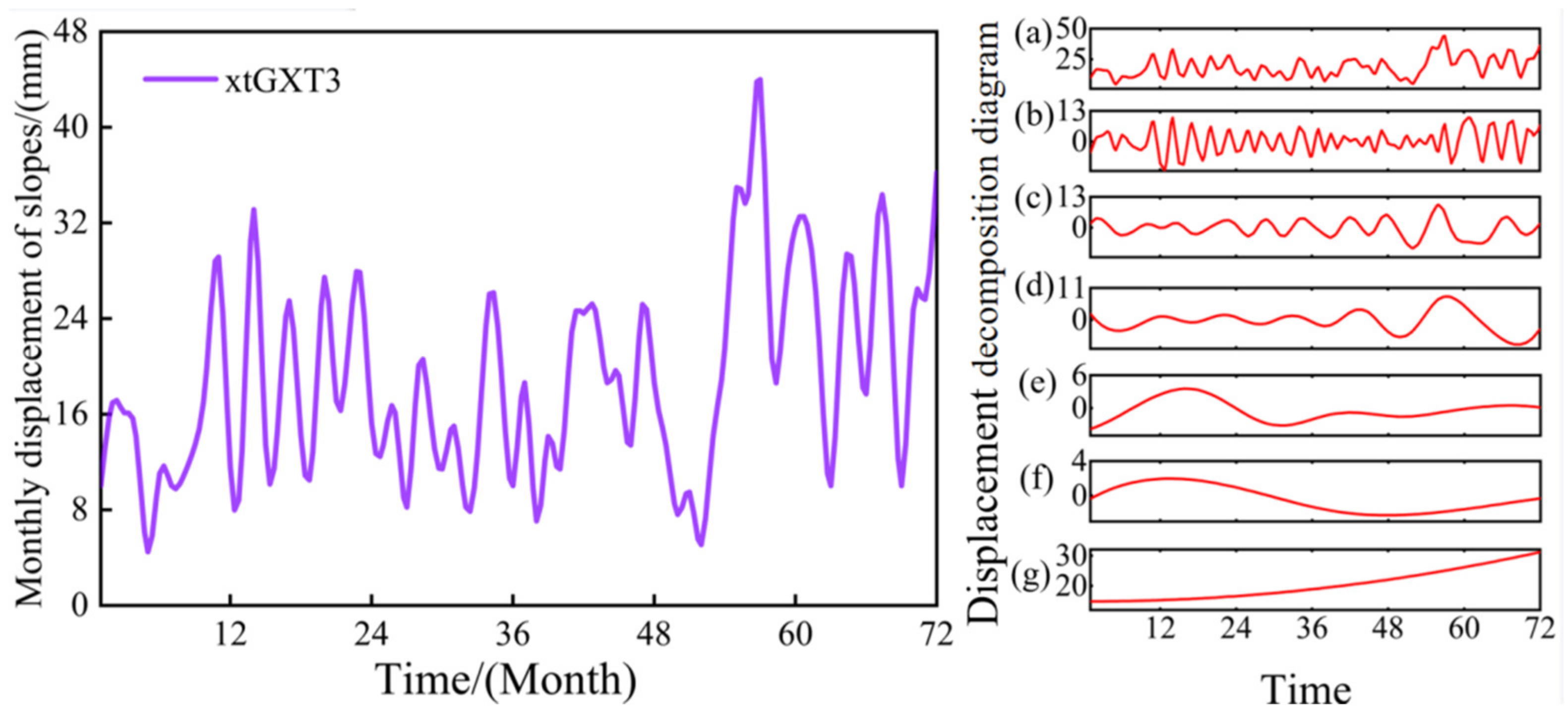
2.1. Empirical Modal Decomposition

Empirical modal decomposition decomposes a complex signal into a sum of multiple intrinsic modal components based on the assumption that any complex signal is composed of multiple distinct components (IMFs) [15]. The core idea of the algorithm is to decompose the complex raw data into a finite number of intrinsic modal functions (IMFs) and residual signals that contain all the fluctuation information of the raw data on the corresponding time scales. Each IMF component must satisfy the following two conditions: the number of poles and the number of cross-zeros are the same or, at most, not equal to one, and the upper and lower envelopes of the component are locally symmetric about the time axis. In this way, any signal can be decomposed into a finite number of IMF sums, and any signal can be decomposed using the EEMD method on this basis. IMFs can be “filtered” as follows:

All local maxima of the signal are found; moreover, all local maxima are connected with three splines to form the upper envelope. All local minima are connected with three splines to form the lower envelope, and the upper and lower envelopes should include all collected data points. The average of the upper and lower envelopes is noted as $m_i$, $x\left(t\right)-m_i=h_i$. Ideally, if $h_i$ is an IMF, then $h_i$ is a component of $x\left(t\right)$. If $h_i$ does not qualify as an IMF, use $h_i$ as the original data and repeat the above steps to obtain the mean of the upper and lower envelope $m_i$, and then determine if it qualifies as an IMF. If not, continue to repeat $k$ times until the conditions in the IMF are met: $h_{i-1}\left(k\right)-m_{i}k=h_{i}k$. Denote $c_1=h_{1}k$, which is part of the signal that meets the IMF condition. The process of decomposing $c_1$ from $x\left(t\right)$ is shown in Equation (1).

$$r_1=x\left(t\right)-c_1$$

(1)

From Equation (1), after decomposing $c_1$, the above process continues to be repeated using $r_1$ as the original data until $x\left(t\right)$ satisfies the second component of the IMF condition $c_2$. The cycle is repeated $n$ times to obtain the second component of the signal that satisfies the IMF condition $x\left(t\right)$.

$$\left\{\begin{array}{l}{r}_1-c_2=r_2\\ \dots \\ r_{n-1}-c_n=r_n\end{array}\right.$$

(2)

$$x\left(t\right)={\displaystyle \sum _{i=1}^n{c}_i+r_n}$$

(3)

From Equation (3), we conclude that the loop ends when it becomes a monotonic function from which no more components satisfying the IMF condition can be extracted. When $r_n$ is the residual function, it expresses the average trend of the signal. Any signal $x\left(t\right)$ can be decomposed using empirical modal decomposition to obtain the IMF component and the residual component $r_n$.

2.2. Sparrow Search Algorithm

The sparrow search algorithm [16] (SSA) is a swarm intelligence optimization algorithm based on the behavior of sparrow populations when foraging and fleeing predators. The sparrow with the highest fitness value in the population is called the discoverer, and it is responsible for searching for food and providing foraging areas and directions. The rest of the sparrows are called joiners, and they follow the discoverer to obtain food and forage according to the information provided by them. The sparrows with the worst fitness values will fly away from the food area and find another place to feed because they cannot obtain food. In the sparrow search algorithm, the identity of the sparrow is related to its ability to find better food. Although the identity may change at any time, the proportion of discoverers and joiners in the population remains constant. Sparrows with sufficient energy reserves will take on the role of the discoverer. Individuals will spy on the discoverers and compete for more food resources to increase predation rates. During foraging, sparrows will immediately send an alarm signal to the population whenever they spot a predator, and all sparrows will engage in anti-predatory behavior. Sparrows that spot a predator are called scouts. SSA simulates the behavior of discoverers for global searches, accessions for local exploration, and the worst-adapted sparrows, as well as the anti-predatory behavior of sparrows to expand the search area.

The equation for the location update of the discoverer is shown in Equation (4).

$$X_{i,j}^{t+1}=\left\{\begin{array}{l}{X}_{i,j}\left(t\right)•\exp \left(-\frac{i}{\alpha \cdot T}\right),R<ST\\ X_{i,j}\left(t\right)+Q•L,R>ST\end{array}\right.$$

(4)

where $t$ represents the current number of iterations, $T$ is the maximum number of iterations, $X_{i,j}$ represents the adaptation value of the $i$th sparrow at the $j$th iteration, $\alpha$ is a random number between (0, 1], $R$ and $ST$ represent the warning and safety values, respectively, $Q$ is a standard normally distributed random number, and $L$ represents a $1\times d$ matrix, where each element of the matrix is 1.

The formula for updating the position of the joiners is shown in Equation (5).

$$X_{i,j}^{t+1}=\left\{\begin{array}{l}Q•\exp \left(\frac{x_{worst}\left(t\right)-X_{i,j}\left(t\right)}{i^2}\right),i>\frac{n}{2}\\ X_p\left(t+1\right)+\left|X_{i,j}\left(t\right)-X_p\left(t+1\right)\right|•A^{+}•L,i\le \frac{n}{2}\end{array}\right.$$

(5)

where $X_p\left(t+1\right)$ is the discoverer’s best position, $X_{worst}\left(t\right)$ is the current global worst position; $A^{+}$ is a row vector whose elements are randomly chosen to be 1 or −1. When $i>n/2$, the follower needs to proceed to other regions; conversely, a better solution should be found at the best position in the current solution.

To enable the model to jump out of the local optima, vigilantes exist at each generation, and the update of the reconnaissance vigilance is shown in Equation (6).

$$X_{i,d}^{t+1}=\left\{\begin{array}{l}X{b}_{i,d}^t+\eta •\left(X_{i,d}^t-X{b}_{i,d}^t\right),f_i\ne f_g\\ X_{i,d}^t+K•\left(\frac{X{b}_d^t-X{w}_{i,d}^t}{\left|f_i-f_w\right|+\epsilon }\right),f_i=f_g\end{array}\right.$$

(6)

where $\epsilon$ is a constant and $\eta$ is a standard normal distribution.

2.3. Good Point Set Optimization

To expedite the search for the global optimum, the initial solution set needs to be generated in a manner that covers as much space as possible. This paper employs the theory of good point sets proposed by Hua Luogeng [17] to generate the initial solution set, thereby ensuring a more uniform distribution of solutions in the search space. The principle of the good point set theory assumes the existence of a unit cube $G_s$ in an $S$ dimensional Euclidean space. If $r\in G_s$

$$P_n\left(k\right)=\left\{\left(\left\{r_1^{\left(n\right)}•k\right\},\left\{r_2^{\left(n\right)}•k\right\},\cdots ,\left\{r_S^{\left(n\right)}•k\right\}\right),1\le k\le n\right\}$$

(7)

By applying certain operations to the cube, we obtain a set of good points (represented by $P_n\left(k\right)$, with $r$ denoting the good points, $n$ representing the number of good points, and $s$ representing the dimension. We select $r=\left\{2\cos \left(2\pi k/p,1\le k\le S\right)\right\}$ (where the equation satisfies $\left(p-3\right)/2\ge S$ and $p$ is the smallest prime number that satisfies this condition) to define the search space, as shown in Equation (8).

$$x_i\left(j\right)=\left(u{b}_j-l{b}_j\right)•\left\{r_j^{\left(i\right)}•k\right\}+l{b}_j$$

(8)

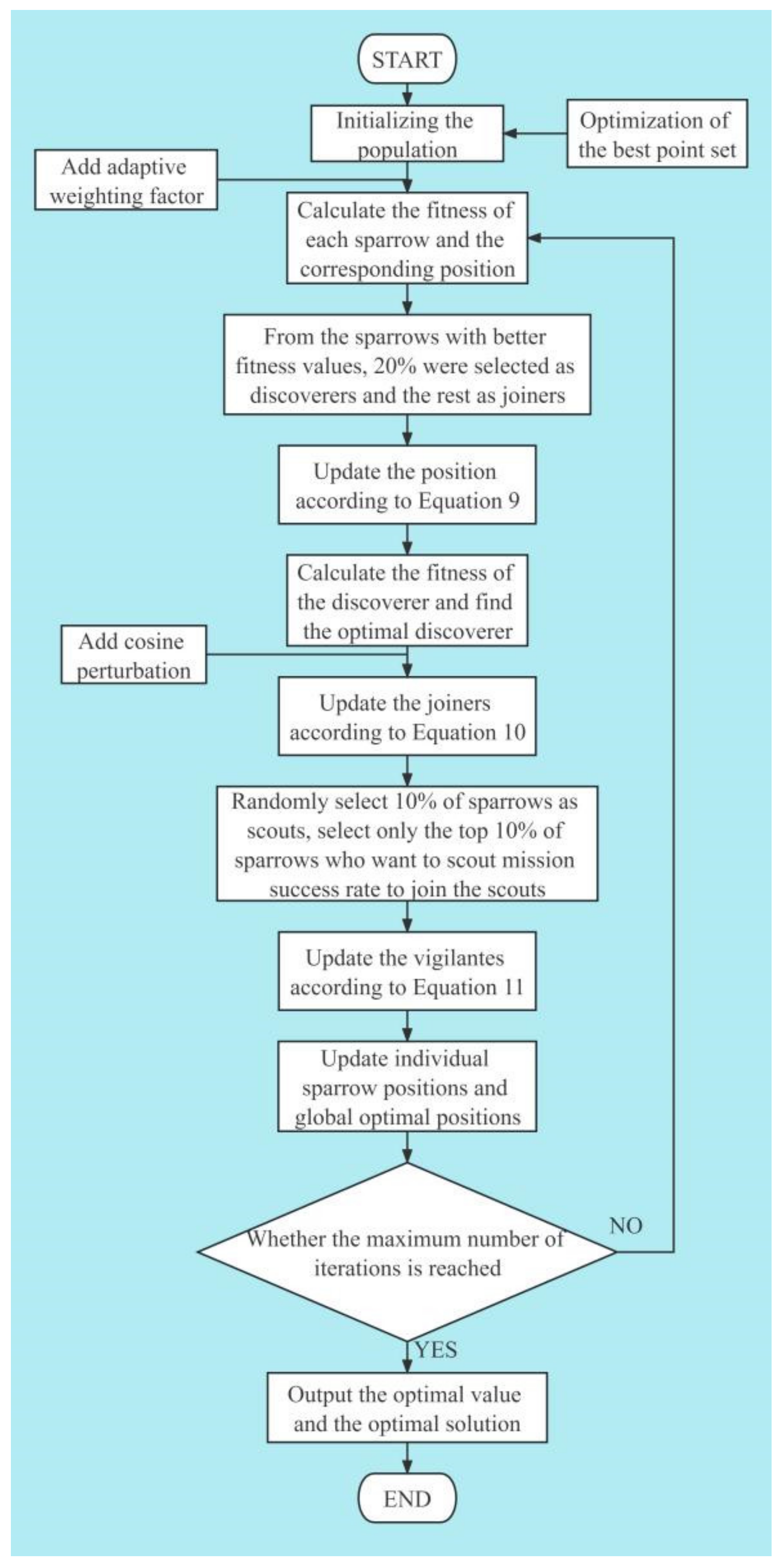
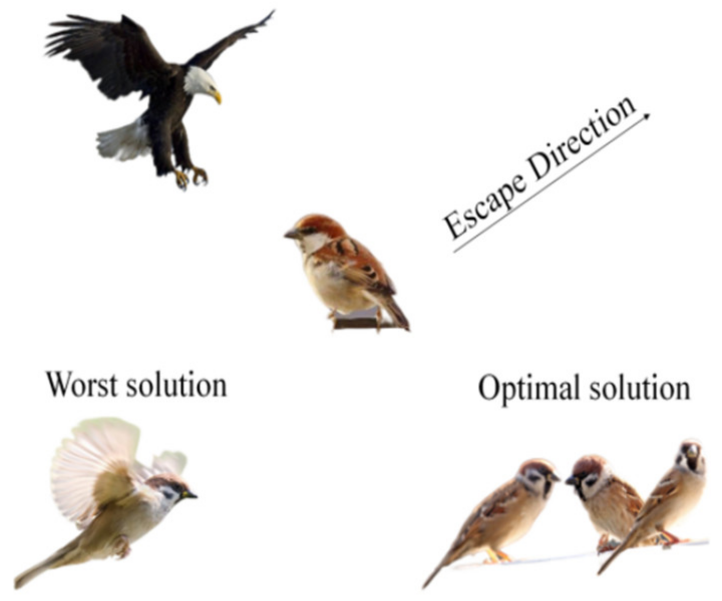
2.4. Irrational Escape Strategy Sparrow Search Algorithm

The sparrow search algorithm (SSA) is known for its high solution speed, convergence accuracy, and stability in engineering applications. However, it can easily fall into a local optimum solution, which may hinder practical engineering applications from converging to the global optimum within a limited number of iterations.

To improve the iteration efficiency, this paper proposes an adaptive weight factor denoted as $\zeta$ in the sparrow algorithm to guide the discoverer to approach the optimal value faster. The optimized discoverer update formula is shown in Equation (9).

$$X_{i,d}^{t+1}=\left\{\begin{array}{l}{X}_{i,d}^t•e^k,R_2\le ST\\ X_{i,d}^t•Q{e}^k,R_2>ST\end{array}\right.$$

(9)

The adaptive weighting factor $\zeta =1/i+1$ is proposed to perform a large area search at the beginning of the computation and accelerate the local optimum search at a later stage compared to the original random convergence approach. To enhance the ability to jump out of the local optimum solution, the cosine perturbation needs to be added to Equation (10) for the follower.

$$X_{i,d}^{t+1}=\left\{\begin{array}{l}\cos \left(2\pi Q\right)•\exp \left(\frac{Q\left(X{\omega }_{i,d}^t—X_{i,d}^t\right)}{i^{\omega }}\right),i>\frac{n}{2}\\ X{b}_d^t+\left|X_{i,d}^t—X{b}_{i,d}^t\right|•A^{+}•L,i\le \frac{n}{2}\end{array}\right.$$

(10)

Furthermore, an irrational method of escape is proposed to accelerate the ability to jump out of the local optimum. The reconnaissance vigilance is updated in Equation (11).

$$X_{i,d}^{t+1}=\left\{\begin{array}{l}X{b}_{i,d}^t+\eta •\left(X_{i,d}^t-X{b}_{i,d}^t\right),f_1\ne f_g\\ X_{i,d}^t+\left(\left(Q\left(X{b}_{i,d}^t-\left|X_{i,d}^t\right|\right)\right)•\sin \left(2\pi Q\right)\right),f_1=f_g\end{array}\right.$$

(11)

where a sparrow in a vigilant position will randomly choose the escape direction and the maximum distance to escape is the distance from the current position to the optimal position using a sinusoidal perturbation. This strategy simulates the behavior of sparrow populations when danger is detected under natural conditions, breaking the rules and escaping from the danger area in an irrational, panicked way. This increases the possibility of the function jumping out of the local optimal solution. The guarded escape method is illustrated in Figure 1. The flow chart of the algorithm is shown in Figure 2.

2.5. Least-Squares Support Vector Machine

The support vector machine (SVM) is a machine learning algorithm based on statistical principles and the principle of structural risk minimization proposed by Vapink et al. [18] in 1995. Its basic idea is to map the original input space data into a high-dimensional feature space via non-linear mapping so that a non-linear regression problem in the original space is transformed into a linear regression problem in the feature space. Support vector machines have a great advantage in solving small sample, non-linear, and high-dimensional problems and can avoid becoming trapped in local optima. Suykens et al. [19] proposed the least squares support vector machine (LSSVM) to improve the support vector machine algorithm, where the inequality constraints in the original SVM training data set are changed to equation constraints in the LSSVM. In the LSSVM model, let the training dataset be denoted by Equation (12).

$$\left(x_i,y_i\right)\in R^n\times R\left(i=1,2,\dots ,l\right)$$

(12)

where $x_i$ denotes the input vector, $y_i$ denotes the output vector, and $l$ denotes the number of samples. In the feature space, the regression function $f\left(x\right)$ can be expressed as:

$$f\left(x\right)={\omega }^T\phi \left(x\right)+b$$

(13)

where $\omega$ denotes the weight vector; $b$ denotes the amount of bias and $\phi \left(x\right)$ denotes the kernel function that projects the input vector to the higher dimensional features. Based on the principle of minimizing the risk of the structure of the algorithm, the function optimization problem can be expressed as:

$$\left\{\begin{array}{l}\underset{\omega ,b,\xi }{\min }\left(\omega ,\xi \right)=\frac{1}{2}{\omega }^T\omega +\gamma \frac{1}{2}{\displaystyle \sum _{i=1}^l{\xi }^2}\\ y={\omega }^T\phi \left(x_i\right)+b+{\xi }_i,i=1,2,\dots ,l\end{array}\right.$$

(14)

where $J\left(\omega ,\xi \right)$ is the construction function; $\gamma$ denotes the penalty parameter and ${\xi }_i$ denotes the $i$th error variable, constructing Lagrange-style solutions.

$$R^{n}L\left(\omega ,b,\zeta ,a\right)=\frac{1}{2}{\omega }^T\omega +\gamma \frac{1}{2}{\displaystyle \sum _{i=1}^l{\xi }_i^2—{\displaystyle \sum _{i=1}^l{\alpha }_i\left({\omega }^T\phi \left(x_i\right)+b+{\xi }_i{y}_i\right)}}$$

(15)

where $R^n\to R^{nh}$ denotes mapping to a vector space of a higher dimension; ${\alpha }_i$ is a Lagrange multiplier and $L\left(\omega ,b,\xi ,\alpha \right)$ is a Lagrange function. This is subject to the following requirements for a partial differential with $\omega ,b,\xi ,\alpha$.

$$\frac{\partial L}{\partial \omega }=0,\frac{\partial L}{\partial b}=0,\frac{\partial L}{\partial {\xi }_i}=0,\frac{\partial L}{\partial {\alpha }_i}=0$$

(16)

It can be found that:

$$\left\{\begin{array}{l}\omega ={\displaystyle \sum _{i=1}^l{\alpha }_i\phi \left(x_i\right)}\\ {\displaystyle \sum _{i=1}^l{\alpha }_i}\\ {\alpha }_i=\gamma {\xi }_i\\ {\omega }^T\phi \left(x_i\right)+b+{\xi }_i—y_i=0\end{array}\right.$$

(17)

According to the Karush–Kuhn–Tucke optimality condition, a linear equation can be obtained as:

$$\left[\begin{array}{cccc}0& 1& \cdots & 1\\ 1& K\left(x,x_i\right)+1/\gamma & \cdots & K\left(x,x_i\right)\\ ⋮& ⋮& \ddots & ⋮\\ 1& K\left(x,x_i\right)& \cdots & K\left(x,x_i\right)+1/\gamma \end{array}\right]\left[\begin{array}{c}b\\ {\alpha }_1\\ ⋮\\ {\alpha }_1\end{array}\right]=\left[\begin{array}{c}0\\ y_1\\ ⋮\\ y_l\end{array}\right]$$

(18)

where $K\left(x,x_i\right)=\phi {\left(x_i\right)}^T\phi \left(x\right)$ is a symmetry function that satisfies the Mercer condition.

2.6. Other Algorithms

2.6.1. Gray Wolf Algorithm

GWO algorithm is an optimization algorithm based on wolf pack collaboration that simulates the process of predatory behavior of gray wolf packs. The algorithm has the advantages of a simple structure, fewer parameter adjustments, and easy implementation. In addition, the GWO algorithm has an adaptively adjusted convergence factor and information feedback mechanism, which can balance local search and global search, and thus shows good performance in terms of solution accuracy and convergence speed.

2.6.2. Particle Swarm Optimization Algorithm

The PSO algorithm is a random search algorithm based on group collaboration, which is inspired by simulating the foraging behavior of a flock of birds. The strategy of this algorithm is as follows: a flock of birds randomly searches for food in a region, and all birds know the distance of their current position from the food; then, the simplest and most effective search strategy is to search the region around the bird that is currently closest to the food. The particle swarm algorithm uses this idea of a bird flock foraging model for inspiration and is applied to solve optimization problems.

2.6.3. Chaotic Sparrow Search Optimization Algorithm

The CSSOA algorithm employs Tent chaos and Gaussian variation techniques. Among them, the Tent chaos perturbation improves the global search ability and the search accuracy; meanwhile, the Gaussian variation has a strong search ability for optimization problems with a large number of local minima and enhances the diversity and robustness of the population. These improvements yield better search performance and pioneering performance for the CSSOA algorithm, improving search accuracy and convergence precision.

3. Algorithm Validation

3.1. Pick Functions

In this paper, we selected three high-dimensional, single-peak benchmark functions; three high-dimensional, multi-peak functions; and three low-dimensional, multi-peak functions to verify the feasibility and accuracy of the IESSA algorithm.

Table 1. Basic information on the three sets of benchmark functions.

Title	Function	Dim	Initial Range	${\mathit{F}}_{\mathbf{min}}$
Unimodal test function	$F_1\left(x\right)={\displaystyle \sum _{i=1}^n{x}_i^2}$	30	[−100, 100]	0
	$F_2\left(x\right)={\displaystyle \sum _{i=1}^n\left|x_i\right|+{\displaystyle \prod _{i=1}^n\left|x_i\right|}}$	30	[−10, 10]	0
	$F_3\left(x\right)={\displaystyle \sum _{i=1}^n{\left({\displaystyle \sum _{j-1}^i{x}_j}\right)}^2}$	30	[−100, 100]	0
Multimodal test function	$F_4\left(x\right)={\displaystyle \sum _{i=1}^n-x_i\sin \left(\sqrt{\left|x_i\right|}\right)}$	30	[−500, 500]	−418.9829 × 5
	$F_5\left(x\right)={\displaystyle \sum _{i=1}^n\left[x_i^2—10\cos \left(2\pi x_i+10\right)\right]}$	30	[−5.12, 5.12]	0
	$F_6\left(x\right)=\frac{1}{4000}{\displaystyle \sum _{i=1}^n{x}_i^2—{\displaystyle \prod _{i=1}^n\cos \left(\frac{x_i}{\sqrt{i}}\right)}}+1$	30	[−600, 600]	0
Fixed- dimension test functions	$F_7\left(x\right)={\left(\frac{1}{500}+{\displaystyle \sum _{j=1}^{25}\frac{1}{j+{\displaystyle \sum _{i=1}^2{\left(x_i-a_{ij}\right)}^6}}}\right)}^{-1}$	2	[−65, 65]	0.998
	$F_8\left(x\right)={\displaystyle \sum _{i=1}^{11}{\left[a_i\frac{x_1\left(b_i^2+b_i{x}_2\right)}{b_i^2+b_i{x}_3+x_4}\right]}^2}$	4	[−5, 5]	0.00038
	$F_9\left(x\right)=-{\displaystyle \sum _{i=1}^4{c}_i\exp \left(-{{\displaystyle \sum _{j=1}^3{a}_{ij}\left(x_j—p_{ij}\right)}}^2\right)}$	3	[1, 3]	−3.75

shows the basic information of the three sets of benchmark functions [20].

To solve the nine benchmark functions, we used the SSA, GWO, CSSOA, PSO, and IESSA algorithms discussed in this paper. Each experiment had a population size of $N$ = 30, a maximum number of iterations $T$ = 100, and assumed that 20% of the population consisted of discoverers and scouts. For each test function, we conducted 30 independent experiments and compared the solutions to derive the mean and standard deviation. We also carried out the optimal solution derived from the coarsening algorithm. The mean value represents the convergence accuracy of the algorithm, and the standard deviation represents the stability of the algorithm, using the same standard test functions. The results of the five algorithms solved are shown in

Table 2. Means and standard deviations of the results of 30 solutions of the three sets of test functions.

	SSA		GWO		PSO		CSSOA		IESSA
	Ave	Std	Ave	Std	Ave	Std	Ave	Std	Ave	Std
F1	2.6 × 10−46	1.4 × 10−45	0.015	0.015	5.80	2.96	1.6 × 10−42	8 × 10−42	0.0	0.0
F2	2.1 × 10−22	9.4 × 10−22	0.023	0.008	6.92	1.68	3.7 × 10−18	2.1 × 10−17	0.0	0.0
F3	5.6 × 10−26	3.1 × 10−25	267.69	178.5	1381.6	543.8	7.5 × 10−31	3.6 × 10−30	0.0	0.0
F4	2.5 × 10−21	1.2 × 10−20	1.467	0.479	5.2355	1.649	1.6 × 10−20	5.1 × 10−20	0.0	0.0
F5	0.003	0.006	30.75	3.50	1917.9	1302.8	0.005	0.013	9.6 × 10−6	1.5 × 10−5
F6	0.0	0.0	0.081	0.061	20.36	4.05	0.0	0.0	0.0	0.0
F7	9.21	4.949	5.282	3.976	3.494	2.751	7.949	5.274	6.324	5.783
F8	3.2 × 10−3	1.6 × 10−4	0.004	0.0075	9.6 × 10−4	1.6 × 10−4	0.0003	6.2 × 10−5	3.1 × 10−4	3.0 × 10−5
F9	10.2	12.14	3.0007	6.9 × 10−4	3	3.1 × 10−13	3	3.4 × 10−10	3	8.0 × 10−9

, including their means and standard deviations.

3.2. Analysis of Results

3.2.1. High-Dimensional Unimodal Test Function

The table shows the results of the 30 solutions for the high-dimensional, single-peak functions (F1–F3). For the single-peak test function, the IESSA algorithm obtains the optimal values of the test functions F1–F3 after zero iterations with a convergence accuracy and standard deviation of 0, which is significantly better than the SSA, GWO, PSO, and CSSOA algorithms. This fully demonstrates that IESSA can obtain more stable and accurate results when solving high-dimensional, single-peak functions. The convergence curve of the single-peak test function is also shown in the figure, and IESSA can quickly arrive at the optimal solution. The IESSA algorithm performs better when dealing with single-peaked test functions.

3.2.2. High-Dimensional Polymodal Test Function

The table shows that, in the process of solving high-dimensional, multi-peaked test functions (F4–F6), the difference between the solution results of IESSA and those of SSA and CSSOA is smaller in the case of test functions F5 and F6 since SSA is better at solving simple functions. However, in the more complex function F4, the convergence accuracy and stability of IESSA in high-dimensional, multi-peaked functions are better than those of SSA and CSSOA. This demonstrates the superior efficiency of the proposed IESSA algorithm.

3.2.3. Low-Dimensional Multipeak Function

The objective function identified in this paper is the low-dimensional, multi-peaked function (F7–F9). As shown in Table 2, the SSA algorithm is less stable, while the CSSOA algorithm has a better ability to jump out of the local solution. However, IESSA employs an irrational escape strategy and achieves better convergence accuracy, stability, and ability to jump out of the local optimal solution than CSSOA in the three selected test functions. Its efficiency is much more than that of SSA, GWO, and PSO.

Apart from stability and convergence accuracy, the convergence speed is also an important factor in evaluating an algorithm’s performance. The convergence speed of IESSA is shown in Figure 3. The number of iterations was set to $T$ = 300, and the rest of the parameters were unchanged. The convergence speed comparison graphs of the three groups function as follows.

In the test functions F1, F2, and F3, IESSA converged much faster than the remaining four algorithms and was able to converge to the optimal value of the function. For test function F4, IESSA exhibited a much higher convergence speed and ability to search for the global optimal solution compared to SSA, GWO, PSO, and CSSOA.

Overall, the IESSA algorithm performed well in the function testing process. Compared with the SSA, GWO, PSO, and CSSOA algorithms, the IESSA algorithm can jump out of the local optimum and then search for the global optimum solution. The convergence speed and accuracy reveal that IESSA has an extremely strong ability to jump out of the local optimum solution; moreover, in terms of the mean standard deviation, the solution accuracy and stability of IESSA are stronger.

4. Engineering Example Application

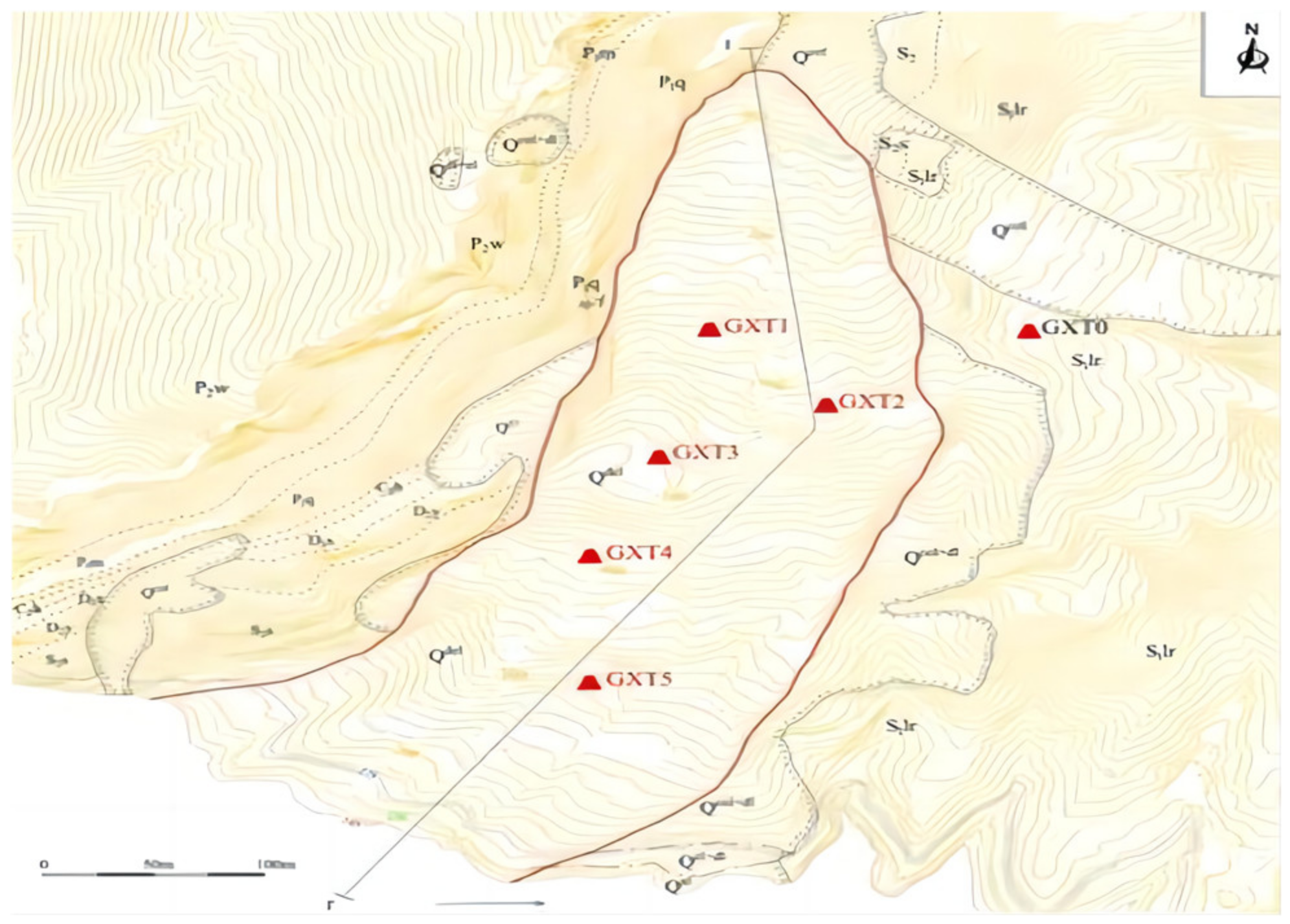
4.1. Hydrogeological Conditions of Xin Tan Landslide

According to meteorological data, annual rainfall in the area of the Xin Tan landslide is relatively abundant, averaging up to 1016 mm. The maximum recorded annual average rainfall reached 1430 mm. The rainfall in the area is particularly abundant during the rainy season, averaging up to 2 mm. The maximum rainfall recorded during the rainy season reached 1107 mm. The rainy season is mainly concentrated between May and September.

The Xin Tan landslide is located on the north bank of the Yangtze River, 26 km away from the Three Gorges Dam site. The body of the Xin Tan landslide is in the shape of a long tongue, the terrain is high in the north and low in the south, and it has a gentle slope inclined to the Yangtze River, with an overall slope degree of 23°. The back edge is located at the foot of Guangjia Cliff, with an elevation of 910 m, and the front edge is located below the water level of 135 m, with a length of 1600 m in the north–south direction, a width of 500 m in the east–west direction, and an average thickness of about 30 m. The landslide surface is the contact surface between the accumulation body and the underlying bedrock. The lithology of the underlying bedrock is Silurian sand–mud shale.

The steep terrain in the landslide area is primarily composed of the Yellow Cliff mountain. The exposed bedrock on the mountain consists mainly of Carboniferous diapiric tuff and Devonian sand and jade. Soluble rocks eroded by water become karst aquifers, while non-soluble rocks experience fissures due to tectonic geological actions, forming fissure aquifers. However, there are also insoluble rocks such as the Wujiaping Formation, Maanshan Section, and Silurian shale in the landslide area, creating a water barrier for the karst and fissure aquifers. Consequently, the groundwater in the aquifers lacks coherence. Moreover, due to the topographic control of the one-sided mountain, most of the surface water and groundwater can only flow into the river along the slope surface in a western direction after atmospheric rainfall reaches the surface. Only a small portion can penetrate into the slope body, resulting in limited recharge to the landslide.

The material on the slope under the Jiangjia slope of the landslide consists mainly of crumbly stone and sandwiched soil formed by the avalanche slope deposit. This type of landslide body has high permeability due to its large porosity. It is widely distributed in the area, and its groundwater source mainly comes from the surface infiltration of atmospheric precipitation. It can also receive recharge from the surface and groundwater from the Huangyan mountain. Although the groundwater source in this area is relatively abundant, the slope body material is composed of gravel soil, which has a larger porosity for groundwater storage. Groundwater circulates through the pores in the slope body material, providing better drainage conditions. Consequently, groundwater does not accumulate significantly, with only a relatively small portion being stored in the grooves formed by impermeable rocks such as sand shale. Additionally, the flow of groundwater from the accumulation area to the river’s front edge is relatively small during the dry season but increases during the rainy season.

4.2. External Factors Affecting Slope Displacement

Among the natural factors that influence slope stability, rainfall, water level, earthquake, and wind play significant roles. Since the effects of earthquakes and wind are minimal for the Three Gorges Xin Tan landslide examined in this paper, and considering that the Xin Tan landslide is situated along the Yangtze River, which typically experiences higher rainfall and increasing water levels with the season, this study focuses on investigating the effects of rainfall and water level as natural factors on the Xin Tan landslide.

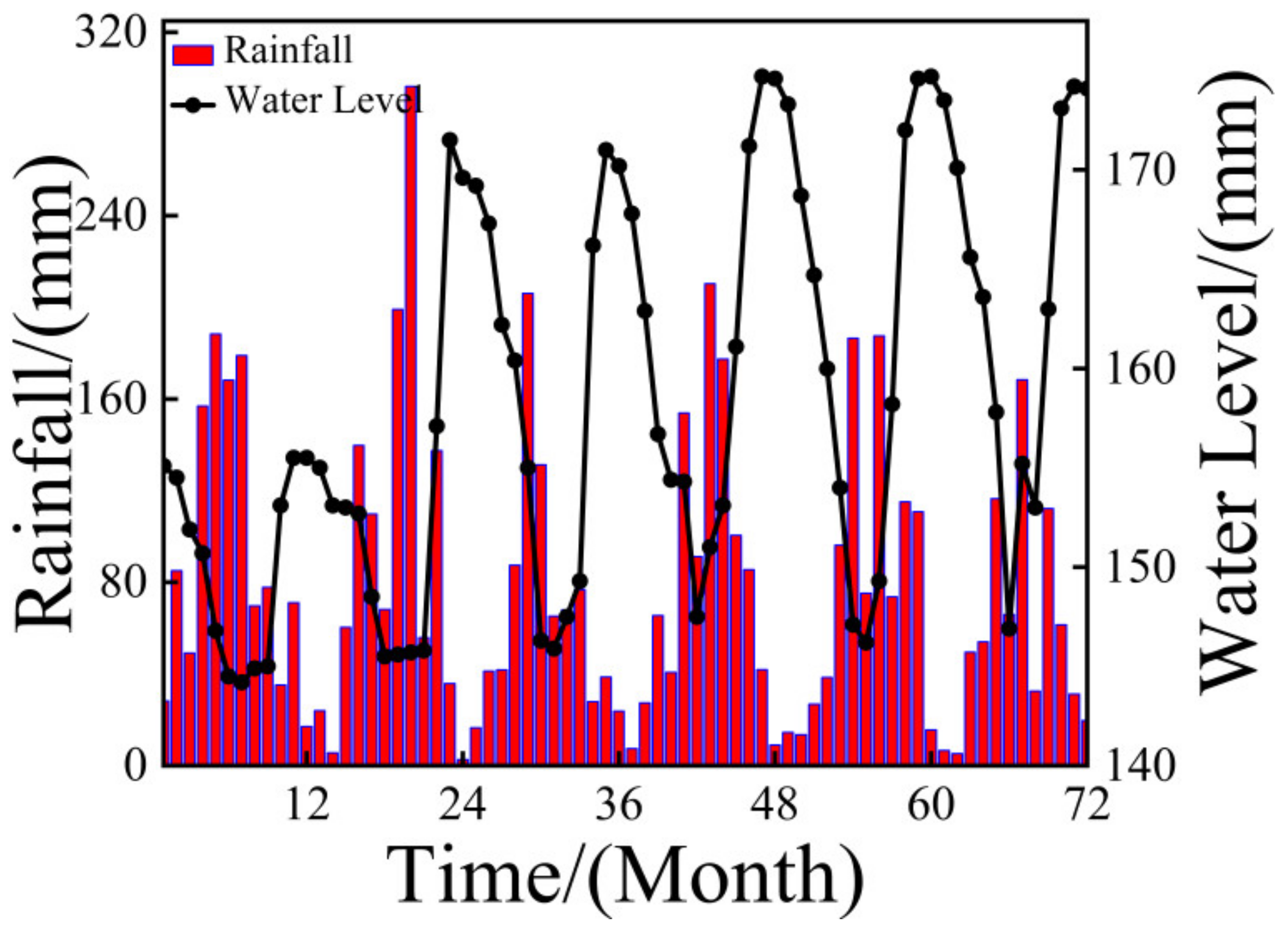
4.2.1. The Effect of Rainfall on Landslides

From a mechanical perspective, the infiltration of rainwater into the slope interior has several effects on slope stability. Firstly, it increases the water content of the soil, thereby raising its capacitance. Additionally, rainwater infiltration generates hydrostatic pressure and dynamic water pressure inside the slope. These pressures exert outward thrust on the slope, leading to an increase in soil sliding force along the potential sliding surface and affecting slope stability.

Prior to rainfall, the pores between the soil particles on the slope are primarily filled with air. During the initial stage of rainfall, raindrops, carrying kinetic energy, cause the dispersion of finer soil particles on the slope surface. As rainfall persists, the water content of the soil on the slope surface gradually increases, replacing the air-filled pores with rainwater and reducing the bonding force between soil particles. Furthermore, continuous rainfall impacts the slope surface, progressively disrupting the original structural state and causing the soil to loosen until it becomes thin mud.

As rainfall continues, water accumulates on the slope surface, resulting in increased flow and runoff intensity. When water flow interacts with the slope, dispersion occurs due to differences in soil structures. Runoff on the slope is unevenly distributed, leading to gully erosion, especially in areas with weak erosion resistance. The energy and scouring capacity of the water flow intensifies, increasing its sediment-carrying force. If the soil’s erosion resistance is lower than the scouring force of the runoff, erosion pits will form. With ongoing rainfall, the scouring capacity of the runoff strengthens, widening the erosion pits and cutting downward towards the foot of the slope, forming small gullies. Continuous rainfall replenishes the slope runoff, further enhancing the water flow’s erosion capacity, which is primarily concentrated in the lower half of the slope. The continuous scouring effect of the water flow gradually undercuts the soil on both sides of the gully trench, eventually leading to local soil destabilization and collapse at the foot of the slope.

4.2.2. The Effect of Water Level on Landslide

During a rise in river level, water infiltrates the slope from the slope surface, causing the water level inside the slope to gradually increase. However, due to soil infiltration, the river level outside the slope rises faster than the water level inside. As a result, hydrostatic pressure is generated inside the slope; meanwhile, dynamic water pressure acts outward from the slope surface. This dynamic water pressure, pointing away from the slope, promotes slope stability.

When the river water level in front of the slope decreases, water continues to seep out from the inside of the slope. The rate of water level decline inside the slope is lower than the rate outside, resulting in dynamic water pressure pointing out of the slope. This, along with a decrease in hydrostatic pressure inside the slope, has a negative impact on slope stability.

Soil permeability also influences slope stability. When the permeability coefficient of the slope soil is low, the groundwater level response in the slope is slower, creating a larger hydraulic gradient. This leads to a larger dynamic water pressure, which adversely affects slope stability. Generally, the influence of dynamic water pressure on slope stability is greater than that of hydrostatic pressure. However, when the water level stabilizes at a normal level, the hydrostatic pressure increases the sliding force of the potential sliding body of the slope. Therefore, when studying slope stability, it is necessary to consider soil permeability, particularly when there are fluctuations in the river water level. Attention should be given to the influence of dynamic water pressure on slope stability.

4.3. Least Squares Support Vector Machine Test

In this study, a total of 72 sets of rainfall, water level, and corresponding displacement data were analyzed. The data were divided into two groups: the training set, consisting of the first 60 sets of data, and the test set, consisting of the remaining 12 sets. To simulate the data set, next, an LSSVM simulation model was established and the sparrow search optimization algorithm was invoked for training. This led to the establishment of the SSA-LSSVM slope displacement simulation model, where the mean square error between the predicted value and the expected value was derived and taken as the initial adaptation value of the sparrow population. However, the SSA-LSSVM algorithm was complicated and time-consuming. Based on the idea of the iterative optimization search, the IESSA-LSSVM algorithm was fused with LSSVM to optimize it. In this algorithm, each sparrow in the sparrow search algorithm is located in the two-dimensional search space ($\gamma ,{\delta }^2$), and the LSSVM calculates the fitness value as the criterion with which to search for the global optimal solution.

4.4. Technology Roadmap

Figure 4 shows that the historical displacement data were input first, followed by decomposing the data into several different signal IMFs using the EEMD method and classifying the IMFs. Next, the support least squares vector machine optimization algorithm with an irrational escape strategy sparrow search algorithm was applied for simulation, and rainfall and water level data were input to fuse the predicted data. Finally, the results of slope displacement prediction were derived, which demonstrated the accuracy of IESSA in slope prediction.

In this study, two factors affecting slope stability, namely rainfall and water level, were selected as input variables, while slope displacement was considered as the output variable. The monitoring points on the Xin Tan slope are depicted in Figure 5. The rainfall and water level data of the monitoring points are shown in Figure 6. Two monitoring points, namely xtGXT1 and xtGXT3 on the Xin Tan landslide of the Yangtze River, were selected as examples, and the monthly displacements of the two slopes were summarized as shown in Figure 7.

The rainfall and water level data at the monitoring sites are as follows:

Figure 6. Rainfall and water level data.

Figure 6. Rainfall and water level data.

Figure 7. Monthly displacement accumulation chart of the slope.

Figure 7. Monthly displacement accumulation chart of the slope.

The EEMD method was used to decompose the data for the two side slopes [21], as shown in Figure 8 and Figure 9.

4.5. Analysis of the Predicted Results

In the regression sequence prediction model, several measures are used to evaluate the prediction accuracy, including the mean absolute error, mean square error, root mean square error, and mean absolute percentage error. To compare the accuracy of different models, we used the root mean square error $\left(RMSE\right)$, mean absolute error $\left(MAE\right)$, the coefficient of determination $\left(R^2\right)$, and mean absolute percentage error $\left(MAPE\right)$ as the accuracy error. The following equation shows the standard for these measures:

$$RMSE=\sqrt{\frac{1}{N}{\displaystyle \sum _{i=1}^n{\left(y_i-\stackrel{\wedge }{y}\right)}^2}}$$

(19)

$$MAE=\frac{1}{n}{\displaystyle \sum _{i=1}^n\left|\left(y_i-\stackrel{\wedge }{y_i}\right)\right|}$$

(20)

$$R^2=1-\frac{{\displaystyle {\sum }_{i=1}^n{\left(y_i-\stackrel{\wedge }{y}\right)}^2}}{{\displaystyle {\sum }_{i=1}^n{\left(y_i-\overline{y}\right)}^2}}$$

(21)

$$MAPE=\frac{100\%}{n}{\displaystyle \sum _{i=1}^n\left|\frac{y_i-\stackrel{\wedge }{y_i}}{\stackrel{\wedge }{y_i}}\right|}$$

(22)

where $y_i$ represents the actual value; ${\stackrel{\wedge }{y}}_i$ represents the predicted value; $\overline{y}$ represents the mean of the true value, and $n$ is the number of samples.

To further verify the generality and credibility of the IESSA-LSSVM algorithm, the LSSVM, SSA-LSSVM, and GWO-LSSVM algorithms were selected to build models for the analysis and prediction of the two slopes—xtGXT1 and xtGXT3—in Xin Tan and the Yangtze River. The number of populations was set to 30, the number of iterations was set to 100, and the dimension was set to 2.

Figure 10 and Figure 11 show the simulation results of the four algorithms, LSSVM, SSA-LSSVM, GWO-LSSVM, and IESSA-LSSVM, over a period of 60 months. The IESSA-LSSVM algorithm resulted in a prediction graph that was much closer to the engineering-measured graph, indicating higher prediction accuracy and better results.

Table 3. Comparison of prediction errors of xtGXT1 slopes using different models.

Model Name	xtGXT1 Side Slope
	RMSE	MAE%	R2	MAPE%
LSSVM	7.4596	7.2644	0.46289	0.64336
SSA-LSSVM	6.9357	4.1177	0.50761	0.29981
GWO-LSSVM	3.496	3.549	0.5636	0.23704
IESSA-LSSVM	0.60002	0.33189	0.98998	0.023009

presents the model error evaluation indicators $MAPE$, $MAE$, $R^2$, and $RMSE$ derived from the four algorithms.

From the table above, it is evident that the error evaluation index values of the IESSA-LSSVM model are better than the other three models, and the error evaluation parameters $RMSE$ and $MAPE$ of the IESSA-LSSVM model are significantly lower than the other three. In the xtGTX1 slope test sample, the IESSA-LSSVM model exhibited a decrease of 6.33568 and 2.89598 in $RMSE$ compared to the SSA-LSSVM and GWO-LSSVM models, respectively. Furthermore, there was a decrease of 0.276801% and 0.2214031% in $MAPE$ and a decrease of 4.084511% and 3.21711% in $MAE$. Moreover, the $R^2$ tended to be more toward 1.

As can be seen from

Table 4. Comparison of prediction errors of xtGXT3 slopes using different models.

Model Name	xtGXT3 Side Slope
	RMSE	MAE%	R2	MAPE%
LSSVM	6.698	6.1595	0.44741	0.35308
SSA-LSSVM	4.0392	4.4196	0.6324	0.26576
GWO-LSSVM	6.0246	5.2036	0.56495	0.30247
IESSA-LSSVM	1.2137	0.67279	0.97714	0.058192

, in the xtGXT3 slope test sample, the IESSA-LSSVM model has much smaller values for $RMSE$, $MAE$, and $MAPE$ than for the remaining three models; meanwhile, $R^2$ is closest to 1, indicating that the model has a small prediction error and a high degree of fit when studying the slope displacements. Therefore, the EEMD-IESSA-LSSVM model proposed in this paper is highly versatile and has high prediction accuracy. However, with the gradual complexity of the algorithm, the model may introduce some errors, but these errors are negligible compared to the model’s accuracy. This model and method can serve as a reference for slope displacement prediction and related forecasting.

4.6. Algorithmic Sorting

Multivariate statistical techniques play a pivotal role in investigating the interrelationships among morphometric parameters and in analyzing algorithmic rankings [22].

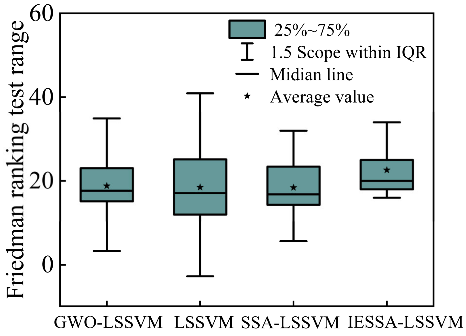
4.6.1. Friedman Ranking Test

The Friedman ranking test was employed to determine if a significant distinction exists between the rankings of these algorithms. If a level of significance is observed (p < 0.05), then the initial hypothesis is rejected, signifying a noteworthy difference between the two datasets. Conversely, if the significance is absent, it indicates a lack of disparity between the data sets. Please import the sample data and refer to the results illustrated in

Table 5. The results of Friedman’s test analysis.

Variable Name	Median	Standard Deviation	P	Cohen’s f-Value
LSSVM	16.791	6.495	0.043	0.13
SSA-LSSVM	17.089	5.16
GWO-LSSVM	17.763	4.858
IESSA-LSSVM	20.046	3.186

and Figure 12.

In the box plot representation, the box delineates the interquartile range, encompassing the central 50% of the data, with the horizontal line signifying the median. A higher median suggests an overall larger dataset. Among the algorithms examined, only the mean of IESSA-LSSVM surpasses 20; meanwhile, its box length is notably compact, implying a concentrated data distribution. This pattern is followed by GWO-LSSVM and SSA-LSSVM. Notably, all four algorithms exhibit quartiles within the normal range, devoid of any outliers. This indicates that IESSA-LSSVM offers superior predictive performance.

Referring to the depicted figure, it becomes evident that the median of IESSA-LSSVM exceeds that of the other three algorithms. Additionally, its standard deviation of 3.186 is smaller compared to the other algorithms. Conversely, the LSSVM algorithm exhibits the smallest median and the largest standard deviation, suggesting its superiority among the four algorithms. The tabulated outcomes of the Friedman’s test analysis display a p-value of 0.043, signifying its statistical significance. This establishes a substantial distinction between GWO, IESSA, LSSVM, and SSA. The magnitude of the discrepancy, as indicated by Cohen’s f-value, stands at 0.13, suggesting a moderate degree of difference.

4.6.2. Nemenyi Test

The Friedman ranking test, by itself, does not suffice to determine the superiority or inferiority of algorithms. To conduct a more comprehensive assessment, the Nemenyi test emerges as a crucial tool for post hoc two-by-two comparisons [23]. The statistical formula employed for calculating the test volume for the comparison between the ith and jth samples is as follows:

$${{\displaystyle \chi }}_{i,j}^2=\frac{{(\overline{{{\displaystyle R}}_i}—\overline{{{\displaystyle R}}_j})}^2}{\frac{N(N+1)}{12}(\frac{1}{{{\displaystyle n}}_i}+\frac{1}{{{\displaystyle n}}_j})C}$$

(23)

$$C=\mathrm{q}\sqrt{\frac{N(N+1)}{6K}}$$

(24)

where c is the corrected statistic, $p$ is the uncorrected statistic, $N$ is the total number of sample observations, $K$ is the number of overall rank orders, $\overline{{{\displaystyle R}}_{\mathrm{i}}}$ is the mean rank of group i, $\overline{{{\displaystyle R}}_{\mathrm{j}}}$ is the mean rank of group j, ${{\displaystyle n}}_i$ is the number of sample instances in group $\mathrm{i}$, ${{\displaystyle n}}_j$ is the number of sample instances in group j, ${{\displaystyle t}}_i$ is the i-th number of same-ranked individuals.

The statistic $\chi$ obeys an x-distribution with degrees of freedom (number of groups − 1), from which the p-value can be obtained and the conclusion drawn.

Nemenyi’s method is a significant approach used for conducting pairwise comparisons. In this context, the algorithms GWO-LSSVM (A), LSSVM (B), SSA-LSSVM (C), and IESSA-LSSVM (D) were subjected to comparison to ascertain the presence of noteworthy differences in their relative standings. The resulting findings have been summarized in

Table 6. The results of Friedman’s test analysis.

Comparison Group	A and B	A and C	A and D	B and C	B and D	C and D
${{\displaystyle \chi }}^2$	6.712	5.340	7.984	1.528	9.403	9.518
P	0.081	0.149	0.02	0.676	0.04	0.042

, provided below:

From Table 6 above, it can be observed that the significance of IESSA-LSSVM, in comparison to the other algorithms, is below 0.05. This suggests a significant distinction between the proposed algorithm and the other three. Notably, GWO-LSSVM and SSA-LSSVM exhibit comparable outcomes in the test. Conversely, the LSSVM algorithm’s performance ranks at the lowest.

Considering factors such as convergence accuracy and speed, a comprehensive ranking of the four algorithms has been formulated and presented in the accompanying table. In the Friedman ranking test, the IESSA-LSSVM algorithm showcased distinctiveness from the remaining algorithms, with a figure exceeding 20 and a standard deviation of 3.18, which is the smallest. In the Nemenyi test, where pairwise comparisons were conducted, the significance of IESSA-LSSVM becomes even more pronounced. When incorporating convergence speed and accuracy into the assessment, the algorithms can be ranked as shown in

Table 7. Algorithmic integrated sorting.

Algorithm Name	Rankings
LSSVM	4
GWO-LSSVM	2
SSA-LSSVM	3
IESSA-LSSVM	1

.

5. Discussion

The process of landslide generation is dynamic and nonlinear. In this paper, the gray wolf algorithm, the sparrow search algorithm, and their optimization algorithms were selected to predict the displacement of two monitoring points in a chosen slope with reasonable accuracy. These models are able to consider the main external factors that contribute to increased landslide displacement during rainfall and water level fluctuations. The model establishes the relationship between the data, specifically the selected rainfall and water level data. By applying machine learning techniques and improving the training accuracy of the test set, the models can predict slope displacement more accurately. These models prove to be valuable tools in slope early warning systems. The study conducted in this paper presents a pioneering analysis compared to previous studies. Instead of using only one monitoring point for each landslide, two monitoring points were utilized, thereby increasing the amount of data available for the machine learning models. This expansion of data is beneficial for achieving better results. However, there are limitations to these models. They do not employ time series analysis, and the significance of rainfall and water level fluctuations over time cannot be thoroughly examined based on the associated factors. Future work will focus on addressing this issue and making further improvements in subsequent stages.

6. Conclusions

In previous studies on slope displacement, many algorithms have been applied to engineering examples. However, most of these algorithms suffer from defects such as slow convergence speed and low convergence accuracy. To optimize the performance of the algorithms, this paper introduces adaptive weight factors and irrational escape strategies to optimize the sparrow search algorithm, thus improving the convergence speed and accuracy. The IESSA algorithm is then applied to function verification and engineering examples, leading to the following conclusions:

(1)

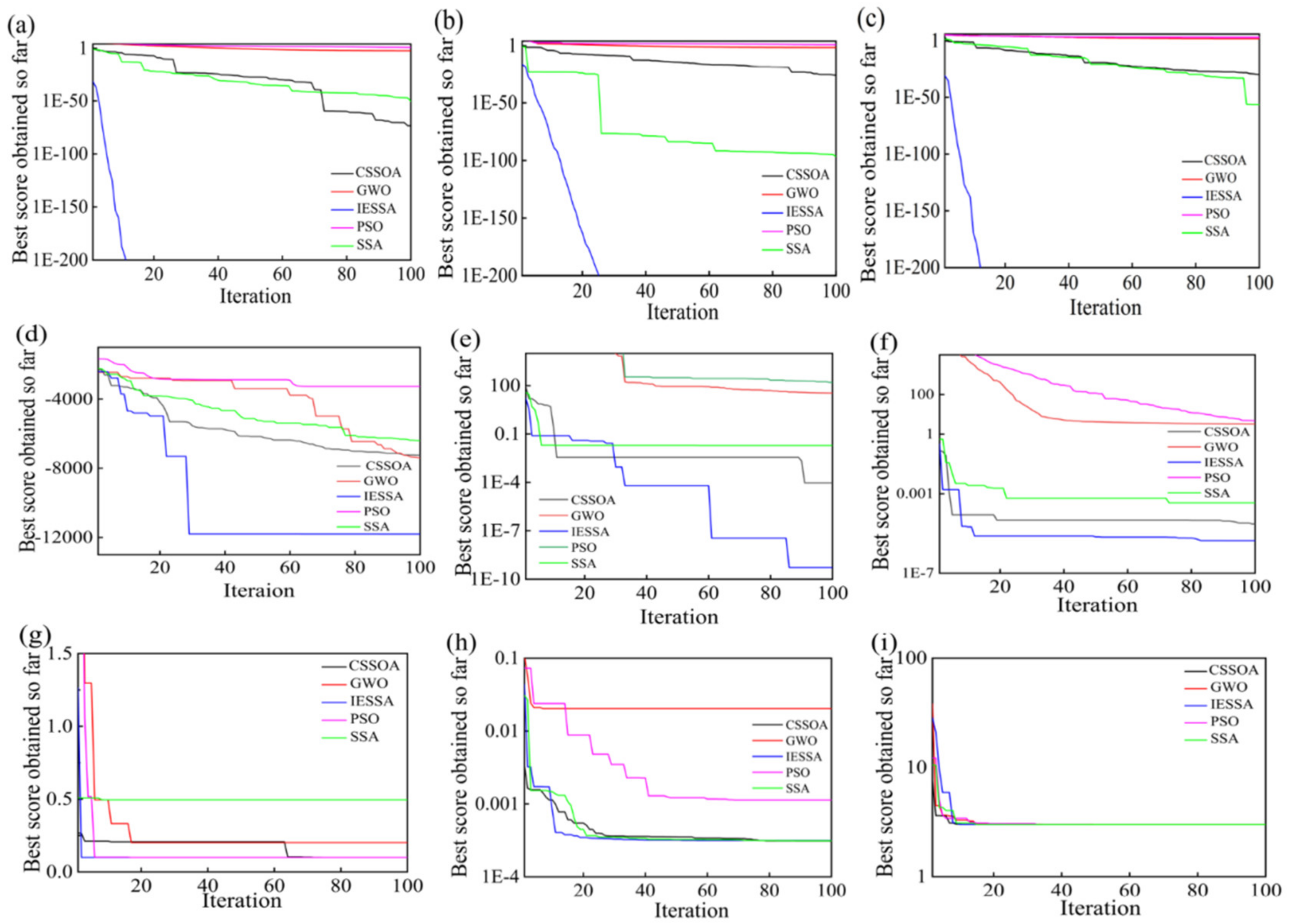
In function verification, the IESSA algorithm performs well in 30 tests of nine benchmark functions, with eight best means and seven smallest standard deviations compared to GWO, SSA, PSO, and CSSOA. In three low-dimensional functions, it has the two best means and the two smallest variances. The root mean square error is the smallest, and the fit is closer to one, indicating that the IESSA algorithm has high accuracy and stability;

(2)

In contrast, the SSA, GWO, PSO, and CSSOA algorithms are prone to fall into local optimal solutions during the iterative process of function verification, making it difficult to perform a global search. The IESSA algorithm proposed in this paper can jump out of the local optimal solution. The iterative adaptation change curve shows that the convergence speed of the IESSA algorithm is much better than the other four algorithms, thus improving the efficiency of function computation;

(3)

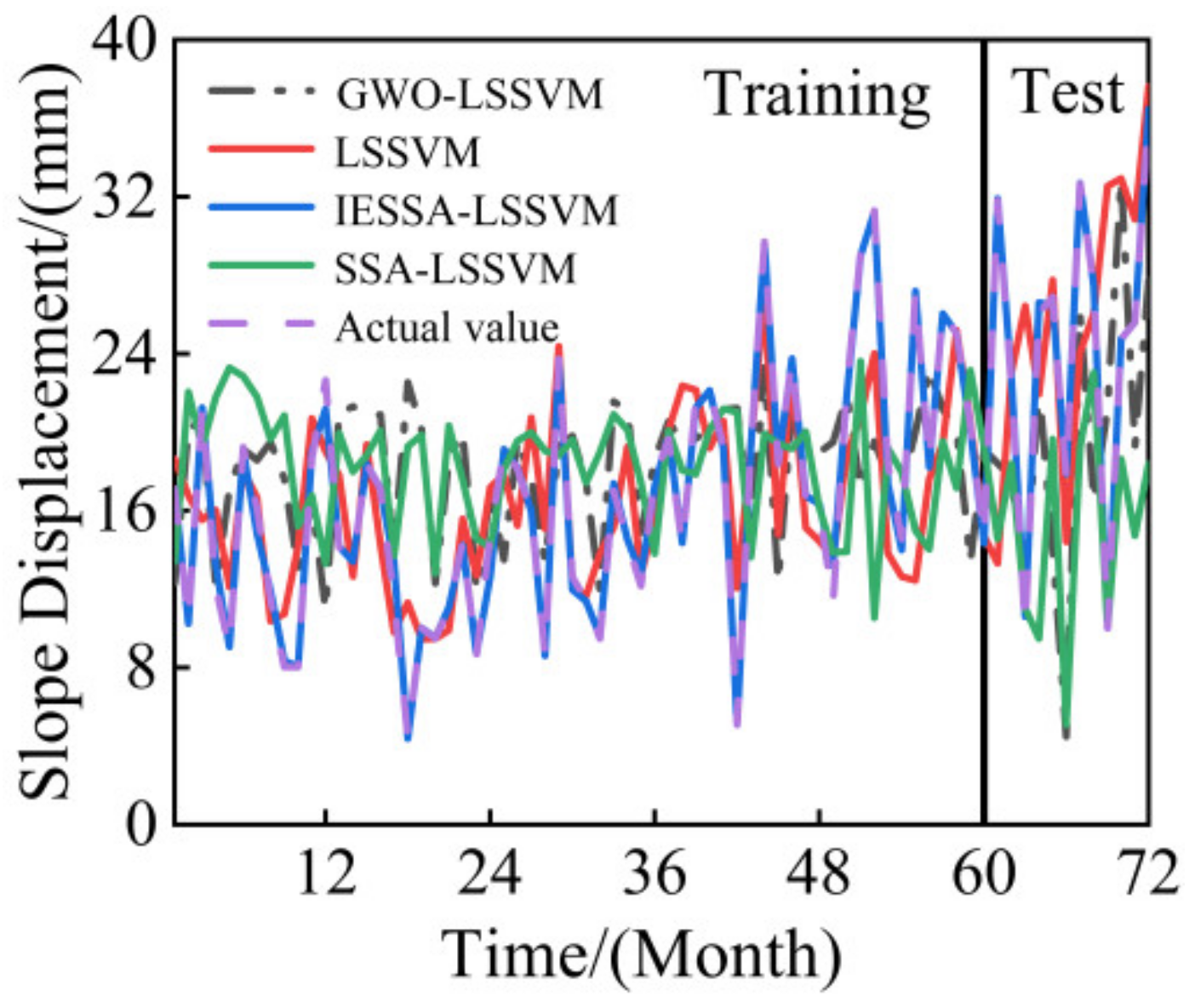
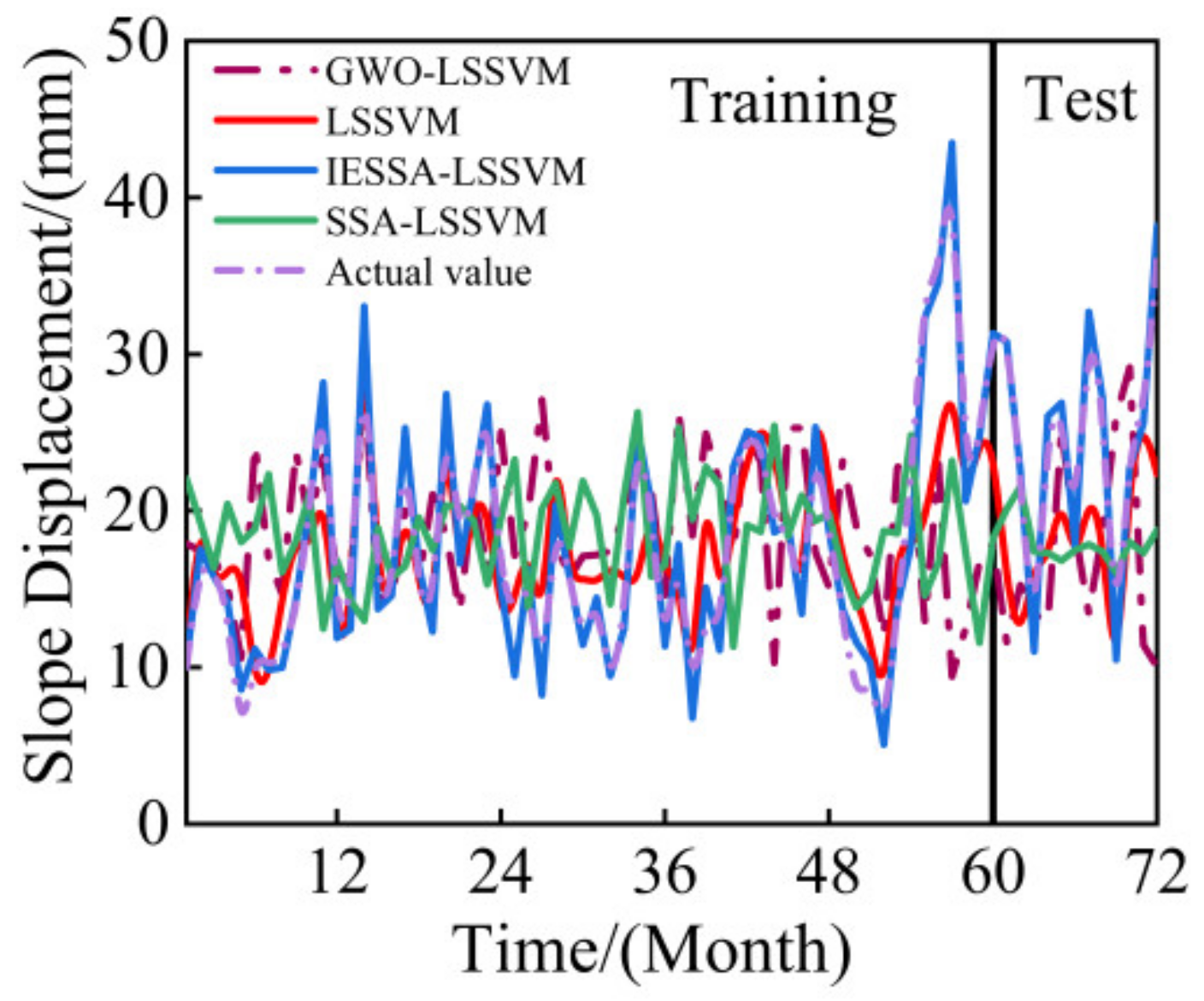
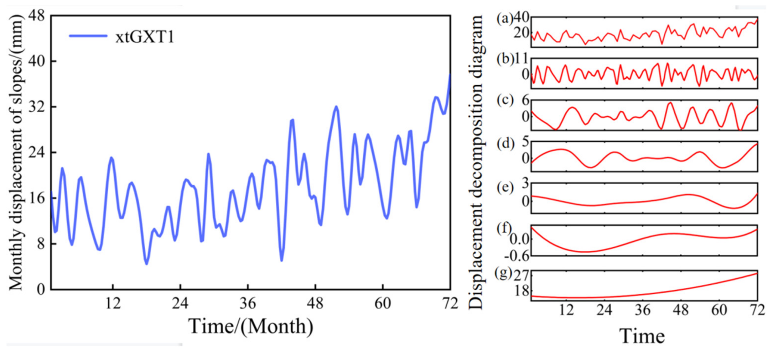
In terms of engineering examples, this paper selects five years of rainfall, water level, and slope displacement data of two new beach slopes—xtGXT1 and xtGXT3—and applies the IESSA algorithm to obtain the slope displacement prediction. The comparison curves show that the IESSA algorithm outperforms the other four algorithms in terms of prediction accuracy. Its root mean square error is the smallest, and the fit is closer to one, indicating the feasibility and accuracy of the IESSA algorithm in engineering examples;

(4)

Considering factors such as convergence accuracy and speed, a comprehensive ranking of the four algorithms has been formulated and presented in the accompanying table. In the Friedman ranking test, the IESSA-LSSVM algorithm showcased distinctiveness from the remaining algorithms, with a figure exceeding 20 and a standard deviation of 3.18, which was the smallest. In the Nemenyi test, where pairwise comparisons were conducted, the significance of IESSA-LSSVM became even more pronounced. When incorporating convergence speed and accuracy into the assessment, the algorithms can be ranked in the following order: IESSA-LSSVM > GWO-LSSVM > SSA-LSSVM > LSSVM.

Overall, the application of IESSA in slope displacement prediction is still at the preliminary exploration stage. More external factors need to be considered to test and optimize the algorithm to verify its feasibility in actual slope displacement prediction.

References

1. Liu, X.; Liu, B. A Hybrid Time Series Model for Predicting the Displacement of High Slope in the Loess Plateau Region. Sustainability 2023, 15, 5423. [Google Scholar] [CrossRef]
2. Huang, F.; Huang, J.; Jiang, S.; Zhou, C. Landslide displacement prediction based on multivariate chaotic model and extreme learning machine. Eng. Geol. 2017, 218, 173–186. [Google Scholar] [CrossRef]
3. Xu, S.; Niu, R. Displacement prediction of Baijiabao landslide based on empirical mode decomposition and long short-term memory neural network in Three Gorges area, China. Comput. Geosci. 2018, 111, 87–96. [Google Scholar] [CrossRef]
4. Wen, T.; Tang, H.; Wang, Y.; Lin, C.; Xiong, C. Landslide displacement prediction using the GA-LSSVM model and time series analysis: A case study of Three Gorges Reservoir, China. Nat. Hazards Earth Syst. Sci. 2017, 7, 2181–2198. [Google Scholar] [CrossRef]
5. Cai, Z.; Xu, W.; Meng, Y.; Shi, C.; Wang, R. Prediction of landslide displacement based on GA-LSSVM with multiple factors. Bull. Eng. Geol. Environ. 2016, 75, 637–646. [Google Scholar] [CrossRef]
6. Herrera, G.; Fernández-Merodo, J.; Mulas, J.; Pastor, M.; Luzi, G.; Monserrat, O. A landslide forecasting model using ground based SAR data: The Portalet case study. Eng. Geol. 2009, 105, 220–230. [Google Scholar] [CrossRef]
7. Huang, F.; Yin, K.; Zhang, G.; Gui, L.; Yang, B.; Liu, L. Landslide displacement prediction using discrete wavelet transform and extreme learning machine based on chaos theory. Environ. Earth Sci. 2016, 75, 1376. [Google Scholar] [CrossRef]
8. Cao, Y.; Yin, K.; Alexander, D.E.; Zhou, C. Using an extreme learning machine to predict the displacement of step-like landslides in relation to controlling factors. Landslides 2016, 13, 725–736. [Google Scholar] [CrossRef]
9. Miao, F.; Wu, Y.; Xie, Y.; Li, Y. Prediction of landslide displacement with step-like behavior based on multialgorithm optimization and a support vector regression model. Landslides 2018, 15, 475–488. [Google Scholar] [CrossRef]
10. Zhou, C.; Yin, K.; Cao, Y.; Ahmed, B. Application of time series analysis and PSO–SVM model in predicting the Bazimen landslide in the Three Gorges Reservoir, China. Eng. Geol. 2016, 204, 108–120. [Google Scholar] [CrossRef]
11. Xing, Y.; Yue, J.; Chen, C.; Qin, Y.; Hu, J. A hybrid prediction model of landslide displacement with risk-averse adaptation. Comput. Geosci. 2020, 141, 104527. [Google Scholar] [CrossRef]
12. Morshed-Bozorgdel, A.; Kadkhodazadeh, M.; Valikhan Anaraki, M.; Farzin, S. A Novel Framework Based on the Stacking Ensemble Machine Learning (SEML) Method: Application in Wind Speed Modeling. Atmosphere 2022, 13, 758. [Google Scholar] [CrossRef]
13. Farzin, S.; Valikhan Anaraki, M. Modeling and predicting suspended sediment load under climate change conditions: A new hybridization strategy. J. Water Clim. Change 2021, 12, 2422–2443. [Google Scholar] [CrossRef]
14. Tiwari, L.B.; Burman, A.; Samui, P. Modelling soil compaction parameters using a hybrid soft computing technique of LSSVM and symbiotic organisms search. Innov. Infrastruct. Solut. 2023, 8, 2. [Google Scholar] [CrossRef]
15. Zhang, K.; Zhang, K.; Bao, R.; Liu, X.-H.; Qi, F.-F. Intelligent prediction of landslide displacements based on optimized empirical mode decomposition and K-Mean clustering. Rock Soil Mech. 2021, 42, 211–223. [Google Scholar] [CrossRef]
16. Xue, J.; Shen, B. A novel swarm intelligence optimization approach: Sparrow search algorithm. Syst. Sci. Control. Eng. 2020, 8, 22–34. [Google Scholar] [CrossRef]
17. Hua, L.G.; Wang, Y. Applications of Number Theory to Approximate Analysis; Science Press: Beijing, China, 1978. [Google Scholar]
18. Cortes, C.; Vapnik, V. Support-Vector Networks. Mach. Learn. 1995, 20, 273–297. [Google Scholar] [CrossRef]
19. Suykens, J.A.K.; Vandewalle, J. Least Squares Support Vector Machine Classifiers. Neural Process. Lett. 1999, 9, 293–300. [Google Scholar] [CrossRef]
20. Mirjalili, S.; Mirjalili, S.M.; Lewis, A. Grey Wolf Optimizer. Adv. Eng. Softw. 2014, 69, 46–61. [Google Scholar] [CrossRef]
21. Wu, Y. Deformation Monitoring Data of Xin Tan Landslide in Zigui County, Three Gorges Reservoir Area, Yangtze River, 2007–2012; National Glacial Permafrost Desert Science Data Center: Lanzhou, China, 2016. [Google Scholar]
22. Sharma, S.K.; Gajbhiye, S.; Tignath, S. Application of principal component analysis in grouping geomorphic parameters of a watershed for hydrological modeling. Appl. Water. Sci. 2015, 5, 89–96. [Google Scholar] [CrossRef]
23. Liu, Y.; Chen, W. A SAS macro for testing differences among three or more independent groups using Kruskal-Wallis and Nemenyi tests. J. Huazhong Univ. Sci. Technol. [Med. Sci.] 2012, 32, 130–134. [Google Scholar] [CrossRef] [PubMed]
Figure 1. Diagram of irrational escape methods.
Applsci 13 09582 g001
Figure 2. Irrational escape strategy optimization sparrow algorithm flow chart.
Applsci 13 09582 g002
Figure 3. Comparison of iteration speed and accuracy of different algorithms. Unimodal test function: (a) F1, (b) F2, (c) F3. Multimodal test function: (d) F4, (e) F5, (f) F6. Fixed-dimension test functions: (g) F7, (h) F8, (i) F9.
Applsci 13 09582 g003
Figure 4. IESSA-LSSVM technology roadmap.
Applsci 13 09582 g004
Figure 5. Schematic diagram of the monitoring point at the Xin Tan landslide.
Applsci 13 09582 g005
Figure 8. EEMD decomposition xtGXT1 side slope map: (a) is the value before the decomposition of the EEMD method, (bg) is the variable decomposed using the EEMD method.
Applsci 13 09582 g008
Figure 9. EEMD decomposition xtGXT3 side slope map: (a) is the value before the decomposition of the EEMD method, (bg) is the variable decomposed using the EEMD method.
Applsci 13 09582 g009
Figure 10. Comparison of xtGXT1 slope displacement algorithm prediction.
Applsci 13 09582 g010
Figure 11. Comparison of xtGXT3 slope displacement algorithm prediction.
Applsci 13 09582 g011
Figure 12. Comparison of Friedman ranking test algorithms.
Applsci 13 09582 g012