MSCSA-Net: Multi-Scale Channel Spatial Attention Network for Semantic Segmentation of Remote Sensing Images

Abstract

Although deep learning-based methods for semantic segmentation have achieved prominent performance in the general image domain, semantic segmentation for high-resolution remote sensing images remains highly challenging. One challenge is the large image size. High-resolution remote sensing images can have very high spatial resolution, resulting in images with hundreds of millions of pixels. This makes it difficult for deep learning models to process the images efficiently, as they typically require large amounts of memory and computational resources. Another challenge is the complexity of the objects and scenes in the images. High-resolution remote sensing images often contain a wide variety of objects, such as buildings, roads, trees, and water bodies, with complex shapes and textures. This requires deep learning models to be able to capture a wide range of features and patterns to segment the objects accurately. Moreover, remote sensing images can suffer from various types of noise and distortions, such as atmospheric effects, shadows, and sensor noises, which can also increase difficulty in segmentation tasks. To deal with the aforementioned challenges, we propose a new, mixed deep learning model for semantic segmentation on high-resolution remote sensing images. Our proposed model adopts our newly designed local channel spatial attention, multi-scale attention, and 16-piece local channel spatial attention to effectively extract informative multi-scale features and improve object boundary discrimination. Experimental results with two public benchmark datasets show that our model can indeed improve overall accuracy and compete with several state-of-the-art methods.

1. Introduction

Remote sensing imagery (RSI) plays a vital role in a wide range of applications, such as land cover, land use, and urban management applications [1,2]. In the past, the semantic segmentation of RSI was mainly carried out with manual methods or traditional machine learning approaches. Manual methods require human analysts to visually interpret the remote sensing imagery and manually delineate the different objects of interest, which is time-consuming, labor-intensive, and subject to human subjectivity and errors. However, human interpretation is often considered reliable due to the expertise and domain knowledge of the analysts.

Traditional machine learning approaches, such as supervised classification algorithms, have also been employed for semantic segmentation of RSI. These approaches involve training a classifier on manually labeled training samples, and then the trained classifier predicts labels for unseen testing samples. Decision trees, support vector machines (SVMs), and random forests are commonly used algorithms.

In recent years, deep learning methods have been successfully used in various fields, such as for facial age estimation [3], super-resolution satellite images [4], clothing retrieval [5], and object identification in satellite images [6,7]. Deep learning has also become a powerful approach for segmentation of RSI [8]. Deep learning-based models, such as convolutional neural networks (CNNs), can learn hierarchical representations directly from the raw images, enabling them to capture complex patterns and spatial dependencies in remote sensing imagery. These models have significantly advanced the accuracy and efficiency of semantic segmentation in RSI. They also have demonstrated superior performance by combining channel, spatial, and contextual information, making them highly effective for extracting detailed and accurate semantic information from remote sensing images.

Semantic segmentation on remote sensing images (RSI) is more challenge than on natural images. The encoder–decoder architectures of SegNet [9] and U-Net [10] are considered the most common semantic segmentation models and mainly fuse feature maps of different scales to obtain more diverse features. In past studies, it can be found that the use of U-Net architecture-based models for semantic segmentation on RSI can help the models to perform segmentation tasks more effectively, but U-Net does not make special adjustments in the connection process, which can also result in the model not fully utilizing the extracted features. Recently, the adaptive focus framework (AF2) [11] was employed with a hierarchical neural network to perform aerial imagery segmentation. The foreground-aware relation network (FarSeg++) [12] has been proposed as a multi-perspective model to alleviate the larger intra-class variance in backgrounds and the foreground–background imbalance in high-spatial-resolution (HSR) remote sensing imagery. The global attention-based fusion network (GAF-Net) [13] adopts a novel fusion architecture to improve performance with remote sensing images.

In response to the aforementioned problems, we propose a new model called MSCSA-Net, which employs two newly proposed modules for effective prediction tasks when it is used in the training stage. The primary contributions of our proposed MSCSA-Net are summarized below.

• More discriminative features: We developed a local channel spatial attention (LCSA) module to extract local feature maps to assist our model in the prediction of the scenes;
• Better recognition and lower computation complexity: We developed a multi-scale attention (MSA) module, which is modified from ASPP [14], to perform separable convolution with different sizes of feature maps with a much lower number of parameters. The MSA can better extract meaningful semantic information to improve the recognition ability of the model without increasing the computation complexity;
• Better features for smaller objects: We developed a 16-piece local channel spatial attention (16-LCSA) module to focus on extracting features for smaller objects to achieve better segmentation accuracy.

2. Related Works

2.1. Deep Learning Models

2.1.1. U-Net

Ronneberger et al. [10] proposed a convolutional neural network called U-Net for segmenting biomedical images. This architecture has been widely used and adapted for various segmentation tasks, including regular image segmentation, medical image segmentation, and remote sensing image segmentation. The U-Net architecture follows an encoder-to-decoder concept, where the encoder is responsible for extracting high-level features from the input image through multiple convolutional and downsampling operations. The downsampling can reduce the spatial resolution of the feature maps while increasing their receptive fields, allowing the network to capture context and global information.

The U-Net architecture also introduces skip connections, which address the problem of information loss during downsampling. By connecting the feature maps from the encoder to the corresponding upsampling layers in the decoder, the network retains access to both high-level and low-level features. This allows the decoder to recover spatial details and contextual information that could have been lost during the downsampling.

In the decoder part of U-Net, the feature maps from the encoder are upsampled using $2\times 2$ upsampling operations. These upsampled feature maps are then concatenated with the feature maps from the corresponding encoder layer, allowing the network to combine both coarse and fine-grained information. This process allows U-Net to generate detailed and accurate segmentation by leveraging both local and global features.

The U-Net design facilitates efficient feature extraction and spatial context integration, making it particularly effective for semantic segmentation tasks, including remote sensing imagery analysis.

2.1.2. ResNet

The residual network (ResNet) [15] architecture is a deep learning model that is primarily composed of residual blocks, and it introduced the concept of residual learning. In traditional deep learning architectures, as the input passes through multiple convolutional layers, information can be lost or degraded due to the vanishing gradient. Residual learning deals with this issue by introducing skip connections (or shortcut connections), which allow the original input features to be added back to the output of a convolutional layer. This residual connection carries the original information directly to the subsequent layers.

By incorporating residual connections, the model can learn to focus on the residual, or the difference between the original input and the feature representation, rather than trying to learn the entire representation from scratch. This enables the model to more effectively capture and utilize fine-grained details and features that may have be lost or difficult to learn through conventional convolutional layers.

The ResNet architecture is named based on the number of layers in the network. For example, ResNet-50 consists of 50 layers, including residual blocks, while ResNet-101 has 101 layers. These deeper architectures have shown improved performance in various computer vision tasks, including facial expression recognition, image classification, object detection, and semantic segmentation.

ResNet and its variants have become popular choices as initial architectures in deep learning models, serving as a foundation for transfer learning and feature extraction in various domains. The use of pre-trained ResNet models, such as ResNet-18, ResNet-50, and ResNet-101, has significantly boosted the performance and efficiency of many computer vision applications.

2.1.3. ResU-Net

The ResU-net [16] architecture combines elements of the ResNet and U-Net architectures to improve semantic segmentation performance. ResU-Net has gained popularity as a basic model for semantic segmentation in various domains.

The ResU-Net architecture consists of two main parts: the encoder and the decoder [2,17,18,19,20,21,22,23]. The encoder part utilizes the ResNet architecture for feature extraction. ResNet’s residual blocks can alleviate the vanishing gradient problem and enable more effective feature learning by incorporating skip connections. By using ResNet as the backbone in the encoder, ResU-Net improves the overall accuracy and feature representation capabilities of the model.

In the decoder part, the architecture adopts the U-Net framework for feature fusion at different scales, as shown in Figure 1. The feature maps extracted from the end of the encoder are progressively fused with the corresponding feature maps from the previous layers in the decoder. This hierarchical fusion allows the model to combine both high-level and low-level features, capturing both global and local information. The fusion process improves the spatial precision and context understanding of the model. The lowest-order feature map is then subjected to further feature fusion, and the final prediction is obtained using a softmax function. This final prediction output represents the segmented regions in the input image.

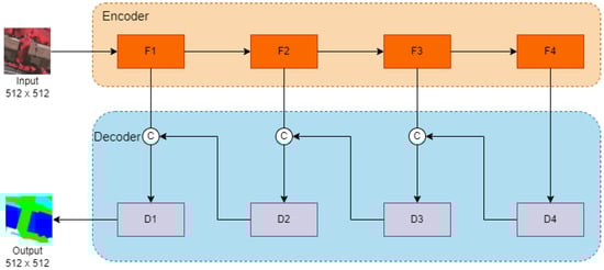
Figure 1. Illustration of the architecture of ResU-Net.The orange part is the encoder, and the blue part is the decoder.

ResU-Net uses ResNet for feature extraction to capture more intricate and detailed features, enhancing segmentation accuracy, and the U-Net-based decoder for feature fusion and contextual understanding, leading to improved segmentation results. ResU-Net has demonstrated better performance compared to the original U-Net architecture in various semantic segmentation tasks across several fields, which has made it a widely adopted and effective model for semantic segmentation.

2.2. Deep Learning-Based Remote Sensing Imagery Methods

2.2.1. SuSA

Kemker et al. [24] proposed a self-taught semi-supervised autoencoder (SSuA) to carry out effective segmentation on satellite images that lack annotations or have limited labeled data, particularly in the context of multispectral imagery (MSI) and hyperspectral imagery (HSI) datasets.

The SSuA first needs to pre-process the input remote sensing image. Then, the authors proposed a stacked multi-loss convolutional autoencoder (SMCAE) to extract meaningful features from the input image. Multiple features are combined, and average pooling is applied to obtain a fused feature representation. The fused feature representation is then fed into the semi-supervised multi-layer perceptron (SS-MLP) architecture. The SS-MLP performs upsampling on the feature map and generates the final prediction segmentation result.

The SSuA approach combines self-learning features and semi-supervised classification to tackle the segmentation task. This approach aims to mitigate the limited availability of labeled data and improve segmentation performance with satellite images.

2.2.2. BiSeNet

Dai et al. [25] proposed an effective water segmentation method called the bilateral segmentation network (BiSeNet) for synthetic aperture radar (SAR) satellite images and established SAR water segmentation data based on GF-3 satellite images.

The BiSeNet architecture first divides the large-scale SAR images into smaller patches of size $512\times 512$. These patches are then categorized into four types based on the pixel intensity ranges: 0–25, 25–50, 50–75, and 75–100. Each patch from the four types is randomly sampled and generated as input with a size of $1024\times 1024$. These input patches serve as the training data for the segmentation network.

BiSeNet consists of two main branches: the spatial path and the context path. The spatial path is responsible for extracting spatial information from the source image and retains the spatial details. The context path, on the other hand, focuses on capturing contextual information and utilizes a lightweight model along with global average pooling to efficiently extract features. The features extracted from the spatial and context paths are fused together. These fused features are passed through a $1\times 1$ convolutional layer, followed by a sigmoid activation function. The sigmoid function maps the output values to the range [0, 1], representing the probability of each pixel being classified as water. After the sigmoid activation, upsampling operations are performed to increase the spatial resolution and generate the final predicted segmentation result.

2.2.3. SCAttNet

Li et al. [2] proposed the spatial and channel attention-based network (SCAttNet) for semantic segmentation of high-resolution remote sensing images. The SCAttNet highlights an aspect of its function by visualizing the learned representations from the spatial and channel attention modules. This visualization provides insights into why the proposed method improves segmentation accuracy, which contributes to the interpretability of the model’s performance.

The experiments were conducted on two benchmark datasets: the ISPRS Vaihingen and Potsdam datasets. The results of these experiments demonstrated competitive performance, especially in handling small objects, which is a significant challenge in remote sensing imagery due to the high level of detail. The authors claim that SCAttNet is a comprehensive approach that could have valuable applications in various remote sensing tasks.

2.2.4. AF2

Huang et al. [11] proposed the adaptive focus framework (AF2) to perform aerial imagery segmentation, which is a specific semantic segmentation task for remote sensing images. The adaptive focus framework (AF2) offers a hierarchical strategy for the segmentation procedure and adaptively utilizes multiscale representations, which are generated by widely used convolutional neural network models.

At each scale’s representation, AF2 introduces a learnable module known as the adaptive confidence mechanism (ACM). This mechanism dynamically assesses the confidence of the scale’s representation for different objects. It dynamically determines which scale of representation is most suitable for segmenting different objects based on their characteristics and complexities. AF2 employs the ACM to filter and select pixels that require accurate segmentation. The mechanism adapts to the specific object characteristics in the imagery and makes decisions on a per-pixel basis regarding the most appropriate representation to use.

AF2 was evaluated on three benchmark datasets, and the results demonstrated that AF2 can significantly improve segmentation accuracy compared to existing methods.

2.2.5. Far Seg++

Zheng et al. [12] introduced a foreground-aware relation network (FarSeg++) to address specific challenges in the segmentation of remote sensing imagery with high spatial resolution (HSR). FarSeg++ aims to mitigate the intra-class variance in backgrounds and reduce the imbalance between foregrounds and backgrounds.

FarSeg++ integrates a relation module for the foreground scene to enhance the discrimination of features for the foreground. This is achieved by considering correlated contexts of the foreground and the linked object–scene relations. This relation-based approach aims to improve the feature representation of the foreground, thereby aiding in accurate segmentation.

The optimization process is foreground-aware, concentrating on foreground examples and challenging background instances during training. This approach strives for balanced optimization in light of the foreground–background imbalance often observed in remote sensing imagery.

To address objectness prediction issues, a decoder is used for dealing with the foreground. This foreground decoder is designed to better represent objectness, which contributes to alleviating problems related to predicting objectness in challenging remote sensing scenarios.

Extensive experiments were conducted to evaluate the robustness and efficiency of FarSeg++. The results indicated that FarSeg++ outperforms state-of-the-art generic semantic segmentation methods. Moreover, FarSeg++ can attain a better balance between segmentation accuracy and speed, which is a practical consideration for many real-world applications.

2.2.6. GAF-Net

Jha et al. [13] introduced the global attention-based fusion network (GAF-Net), which offers an innovative architecture for improving the results of remote sensing image analysis. GAF-Net incorporates global attention mechanisms and introduces cross-attention and self-attention learning techniques.

GAF-Net comprises two types of primary sub-networks:

(1)

Modality-specific classification networks: Two separate networks are designed for each modality. These networks specialize in feature extraction and classification for individual modalities;

(2)

Bi-stream fusion network: The bi-stream fusion network is responsible for combining the outputs of the modality-specific networks and facilitating effective fusion.

GAF-Net introduces a novel self-attention block known as the non-local spectral-spatial self-attention block (SAB). This block plays a pivotal role in capturing long-range dependencies and spatial relationships within the data. GAF-Net also employs cross-attention learning, a technique that enables the network to learn from multiple viewpoints and perspectives. Cross-attention mechanisms help in integrating information from different sources, allowing the network to make well-informed decisions.

3. Proposed Method

We propose a new end-to-end neural network model called the multi-scale channel spatial attention network (MSCSA-Net) for semantic segmentation of remote sensing images. The architecture of MSCSA-Net is depicted in Figure 2a and was mainly inspired by the encoder–decoder architecture.

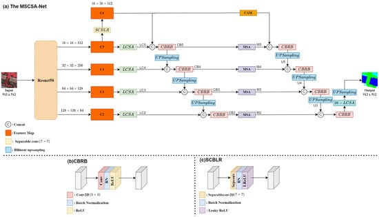
Figure 2. (a) The overall architecture of MSCSA-Net. (b) The CBRB module in MSCSA-Net. (c) The SCBLR module in MSCSA-Net.

In the encoder, ResNet-50 is used as our backbone to extract four different scales of feature maps, which are obtained after maxpooling layers. We name the four different scales of feature maps as C2, C3, C4, and C5, as shown in the figure. The higher-level feature map C5 is passed through the separable convolution batch normalization leaky ReLu (SCBLR) block to obtain feature map C6. The architecture of the SCBLR block is shown in Figure 2c. The input feature map C5 is passed through the 2D separable convolution of kernel size $7\times 7$ and then goes to the batch normalization and leaky ReLu layers to generate output feature map C6.

For the decoder, we can divide it into two parts. The first part uses our proposed local channel spatial attention (LCSA) module on four of the feature maps (C2 to C5). The LCSA module is depicted in Figure 3 and introduced in detail in Section 3.1.

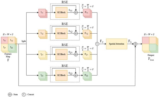
Figure 3. The architecture of the local channel spatial attention (LCSA) module.

The feature map C5 is passed through LCSA module and the LCSA output LC5 is concatenated with feature map C6. The concatenated feature map is then passed through the convolution batch normalization ReLu block (CBRB) for output CB5, where the kernel size of the CBRB is $3\times 3$. The architecture of the CBRB is shown in Figure 2b. The CBRB output CB5 is upsampled and concatenated with the LCSA output LC4, and then it is passed through the CBRB for output CB4. The CBRB output CB4 is upsampled and concatenated with the LCSA output LC3, and then it is passed through the CBRB for output CB3. The CBRB output CB3 is upsampled and concatenated with the LCSA output LC2, and then it is passed through the CBRB for output CB2.

In the second part of the decoder, we use our proposed multi-scale attention (MSA) module, which can be treated as another decoder. The CBRB outputs CB5, CB4, CB3, and CB2 are passed through MSA modules to generate MSA outputs M5, M4, M3, and M2, respectively. The feature map C6 goes to the channel attention module (CAM) and its output is concatenated with the MSA output M5 and then passed through the CBRB and upsampled for output U5. The MSA output M4 is concatenated with the upsampled output U5, and then it is passed through the CBRB and upsampled for output U4. The MSA output M3 is concatenated with the upsampled output U4, and then it is passed through the CBRB and upsampled for output U3. The MSA output M2 is concatenated with the upsampled output U3, and then it is passed through the CBRB and 16-LCSA and upsampled for the final prediction output.

3.1. Local Channel Spatial Attention (LCSA)

The architecture of the local channel spatial attention is depicted in Figure 3.

Although the overall feature map can be effectively enhanced via global channel attention, the local feature enhancement is even more important when RSI is considered. Therefore, as shown in Figure 3, we propose local channel spatial attention (LCSA), a local feature enhancement module, to explore the local area of RSI. In the experiments, the proposed LCSA proved to be more beneficial than global channel attention and could further improve prediction accuracy.

The operation of the LCSA is addressed below. First, as depicted in Figure 3, the input global feature map F is split into four local feature maps $f_{11},f_{12},f_{21}$, and $f_{22}$, as described in Equation (1). F is the original feature map of size $H\times W\times C$, where H, W, and C are the height, width, and channel number of the feature map, respectively. The split local feature $f_{x,y}$ has the size $\frac{H}{2}\times \frac{W}{2}\times C$, where $x=1,2$ and $y=1,2$.

$$F=\left[\begin{array}{cc}{f}_{11}& f_{12}\\ f_{21}& f_{22}\end{array}\right]$$

(1)

Then, the split local feature $f_{x,y}$ enters the squeeze and excitation (SE) block [26], and the split local feature $f_{x,y}$ is added with the SE block output $S_{x,y}$ to generate the residual SE (RSE) block output $R_{x,y}$, where $x=1,2$ and $y=1,2$. As shown in Equation (2), the $S_{x,y}$ is the feature after the SE block, and $\sigma$ denotes sigmoid. The RSE block output $R_{x,y}$ is the sum of the SE output and the input feature, as shown in Equation (3), and each has a size of $\frac{H}{2}\times \frac{W}{2}\times C$.

$$S_{x,y}=\sigma \left(\frac{1}{h\times w}\sum _{i=1}^h\sum _{j=1}^w{f}_{x,y}\right)$$

(2)

$$R_{x,y}=f_{x,y}+S_{x,y}$$

(3)

Next, the four RSE block outputs are combined to restore the original spatial size, as shown in Equation (4).

$$F_c=\left[\begin{array}{cc}{R}_{11}& R_{12}\\ R_{21}& R_{22}\end{array}\right]$$

(4)

The restored global feature $F_c$ is sent to the spatial attention for further feature enhancement. The architecture of our designed spatial attention is depicted in Figure 4.

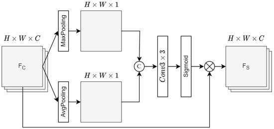
Figure 4. The architecture of the spatial attention (SA).

As described in Equation (5), it first performs max-pooling and average-pooling on $F_c$, and $MaxPool\left(F_c\right)$ and $AvgPool\left(F_c\right)$ are concatenated. Then, it performs convolution on the concatenated feature $Cat\left[MaxPool\left(F_c\right),AvgPool\left(F_c\right)\right]$ and is activated by the sigmoid function. The sigmoid-activated feature is multiplied with the input feature $F_c$ to generate the output feature $F_s$.

$$F_s=\sigma \left(Conv2D\left[MaxPool\left(F_c\right),AvgPool\left(F_c\right)\right]\right)\times F_c$$

(5)

Finally, as shown in Equation (6), the feature maps $F_s$ and F are added to obtain the LCSA output $F_{lcsa}$.

$$F_{lcsa}=F_s+F$$

(6)

3.2. Channel Attention Mechanism (CAM)

The channel attention mechanism (CAM) [27] is a channel feature enhancement module for the feature tensor and it can help the feature map obtain more channel-focused features from it. Our modified CAM architecture is shown in Figure 5, which is different from the general channel attention mechanism.

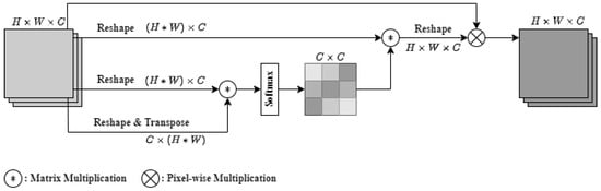
Figure 5. Illustration of the architecture of the CAM.

This modified CAM uses reshape to reorder the feature maps on three branches. The third branch uses transpose to perform matrix multiplication with the second branch and the softmax function to obtain the feature tensor of $C\times C$. Then, the feature tensor of $C\times C$ is multiplied with the reshaped feature from the first branch to obtain the enhanced channel feature tensor. Finally, the enhanced channel feature tensor is multiplied by the input feature for the output.

3.3. Multi-Scale Attention (MSA)

Our proposed multi-scale attention (MSA) module was derived by modifying the atrous spatial pyramid pooling (ASPP) model with improvements. The architecture of the multi-scale attention (MSA) module is depicted in Figure 6.

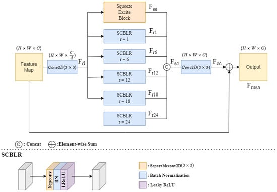
Figure 6. Illustration of the architecture of the multi-scale attention (MSA) module.

The input feature map is passed through a $3\times 3$ convolution with a channel reduction rate d applied to the channel number, which aims at reducing the dimensionality of the feature map, to obtain the dimension-reduced feature $F_d$. The $F_d$ is passed through an SE block and five separable convolution batch normalization leaky ReLu (SCBLR) blocks with five different dilation rates (r = 1, 6, 12, 18, 24) to obtain different scales of receptive fields. The SCBLR block is also shown in the lower part of Figure 6, and it is formed of a separable convolution layer with kernel size $3\times 3$, a batch normalization layer, and a leaky ReLu layer.

Then, the SE block output $F_{se}$ and five SCBLR block outputs $F_{r1},F_{r6},F_{r12},F_{r18},F_{r24},$ are concatenated in the channel to form a size-restored feature $F_{sc}$, which is passed through a convolution layer with kernel size $3\times 3$ to obtain feature $F_{cc}$. The feature $F_{cc}$ is added to the input feature to generate the MSA output feature $F_{msa}$.

3.4. Sixteen-Piece Local Channel Spatial Attention (16-LCSA)

We propose a 16-piece local channel spatial attention (16-LCSA) module to further explore the properties of local features. The architecture of the 16-LCSA module is shown in Figure 7. The operation of the 16-LCSA module is described below.

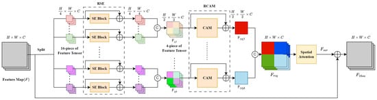
Figure 7. Illustration of the architecture of the 16-piece local channel spatial attention module.

The input feature map is split into 16 equal patches and each patch enters a residual squeeze and excitation (RSE) block. Then, the 16 RSE outputs are merged in groups of four to obtain four-piece features $F_{q1},F_{q2},F_{q3},F_{q4}$. These four-piece features are passed through the residual CAM (RCAM) to get the RCAM-enhanced features $F_{cq1},F_{cq2},F_{cq3},F_{cq4}$.

The residual channel attention features are combined into a restored feature $F_{rcq}$ with the same dimensions as the input feature. The restored feature $F_{rcq}$ is sent to the spatial attention to obtain feature $F_{sar}$, which is added to the input feature to obtain the 16-LCSA output feature $F_{16sa}$.

4. Experiments and Discussion

The experiments were conducted using two public benchmark datasets. We introduce these two datasets and provide a discussion of the experimental results.

4.1. Datasets

The ISPRS Vaihingen dataset is provided by the International Society for Photogrammetry and Remote Sensing (ISPRS) and includes multi-category semantic segmentation satellite images of the German town of Vaihingen. It provides 33 images with various sizes ranging from $1996\times 1995$ pixels to $3816\times 2550$ pixels, and the ground sampling distance (GSD) is 9 cm.

The Vaihingen dataset has six categories marked with different colors, and these six categories and their corresponding colors are impervious surfaces (white), buildings (blue), low vegetation (light blue), trees (green), cars (yellow), and background (red). Near-infrared (IR), red (R), and green (G) channels, together with the digital surface model (DSM), are provided in the dataset. In our experiments, we followed the dataset split setting. Sixteen images were used in the training/validation phase and seventeen images in the testing. We cropped them to a size of $512\times 512$ pixels. After cutting, the total number of training and validation samples was 2550, and the number of test samples was 2400.

The ISPRS Potsdam dataset is also provided by the ISPRS and has multi-category semantic segmentation satellite images of the German town of Potsdam. It provides 38 images of $6000\times 6000$ pixels and the GSD is 5 cm. The Postdam dataset provides six categories marked with different colors, and these six categories and their corresponding colors are impervious surfaces (white), buildings (blue), low vegetation (light blue), trees (green), cars (yellow), and background (red). IR, R, and G channels, together with the DSM, are provided in the dataset. In the experiments, we also followed the dataset split setting. Twenty-four images were used in training/validation and fourteen images in testing. We also cropped them to a size of $512\times 512$ pixels. After cropping, the total number of training and validation samples was 3042, and the number of test samples was 1989.

The reason for choosing the ISPRS Vaihingen and Potsdam datasets for our experiments was that they are more challenging because their use of urban telemetry images can increase the difficulty of the segmentation task. This challenging characteristic make them suitable for the research. However, the bias in these two datasets is that the background area is relatively large compared to other categories.

The ISPRS Vaihingen and Potsdam datasets are both available online at https://www.isprs.org/education/benchmarks/UrbanSemLab/default.aspx (accessed on 4 June 2023).

4.2. Evaluation Metrics

The performance of our proposed MSCSA-Net with these two datasets was evaluated by using the mean intersection over union (mIoU) and F1-score (F1). The mIoU and F1-score are commonly used in evaluating performance in segmentation tasks, and they can help us understand the differences between our segmentation results and the ground-truth pixels.

$$\begin{array}{c}\hfill mIoU=\frac{1}{n}\sum _{i=1}^n\frac{T{P}_i}{T{P}_i+F{P}_i+F{N}_i}\end{array}$$

(7)

$$\begin{array}{c}\hfill F1=2\times \frac{Precision\times Recall}{Precision+Recall}\end{array}$$

(8)

$$\begin{array}{c}\hfill Precision=\frac{TP}{TP+FP}\end{array}$$

(9)

$$\begin{array}{c}\hfill Recall=\frac{TP}{TP+FN}\end{array}$$

(10)

where $T{P}_i$, $F{P}_i$, and $F{N}_i$ indicate the true positives, false positives, and false negatives for an object indexed with class i, respectively. The F1-score and mIoU were calculated for all categories.

4.3. Experimental Setting

In our experiments, we used an Nvidia RTX 3090 GPU for training, validation, and testing. For the training and validation phases, 100 epochs were set for learning convergence. The focal loss [28] was selected for the loss function during the experiments. This loss function helped our model adjust the weights for difficult and simple samples to balance the problem of uneven numbers of difficult and simple samples. The learning rate was set to ${10}^{-4}$, which was more stable for the model training and validation. Due to the limits of the GPU memory, the batch size was set to 4. During training and validation, 80% of the training data were randomly selected for training and the remaining 20% were for validation.

$$\begin{array}{ccc}\hfill L_{focal}& =& \hfill -\alpha {\left(1-p\left(y_t\right)\right)}^{\gamma }log\left(p\left(y_t\right)\right)\hfill \end{array}$$

(11)

4.4. Ablation Study

We conducted ablation studies on the ISPRS Vaihingen and Potsdam datasets to demonstrate the rationality and effectiveness of each module of our proposed MSCSA-Net. The listed results for each category are shown in terms of the F1-score.

Analysis of results for ISPRS Vaihingen. Table 1 lists the segmentation results for the test set with the Vaihingen dataset. In the first row, the results were obtained by using ResU-Net, and these results were used as the baseline results.

Table 1. Ablation study with the Vaihingen dataset. The F1-score was used as the evaluation metric for each category. The overall results were evaluated using the m-F1-score and mIoU. The bold number means the best performance among all methods.

Methods	Params (M)	Impervious Surfaces (F1)	Buildings (F1)	Low Vegetation (F1)	Trees (F1)	Cars (F1)	m-F1	mIoU
ResU-net (baseline) [16]	39.1	72.1	76.0	53.9	67.3	39.4	67.1	50.5
MSCSA-Net without attention	41.0	84.5	86.6	69.9	70.9	68.7	80.8	67.8
MSCSA-Net without LCSA	45.3	81.9	87.4	65.4	77.5	25.1	77.8	63.6
MSCSA-Net without MSA	83.3	80.5	86.3	63.5	75.8	11.9	76.1	61.5
MSCSA-Net without 16-LCSA	87.2	85.4	90.1	71.0	81.6	60.4	81.9	69.4
MSCSA-Net (d = 4)	87.4	85.4	90.2	72.3	82.5	62.5	82.4	70.1
MSCSA-Net (d = 1)	91.7	85.7	90.5	74.2	82.7	61.8	83.0	70.9

The second row shows the results of our proposed model without any of our designed attention modules (no LCSA, no MSA, no 16-LCSA). Compared with the results shown in the first row, one can see that the F1-scores for five categories (impervious surfaces, buildings, low vegetation, trees, and cars) were all higher than ResU-Net. The m-F1-score and mIoU were also better than ResU-Net. This means we could simply use our MSCSA-Net without attention modules to achieve better results than ResU-Net.

Then, we adopted any two of the attention modules in our proposed model. The third row shows the results for our proposed model without the LCSA module. The fourth row shows the results for our proposed model without the MSA module. The fifth row shows the results for our proposed model without the 16-LCSA module. These results were indeed better than for ResU-Net. Among these three methods, the MSCSA-Net without the 16-LCSA module had the best performance, and it had m-F1 = 81.9 and mIoU = 69.4. This shows that one can use two of our designed attention modules, LCSA and MSA, and achieve higher m-F1-score and mIoU.

The sixth and seventh rows show the results for our proposed MSCSA-Net model with MSA channel reduction rates of $d=4$ and $d=1$, respectively. It can be seen that MSCSA-Net ($d=4$) had the second best m-F1-score (82.4) and the second best mIoU (70.1). MSCSA-Net ($d=1$) had the best m-F1-score (83.0) and the best mIoU (70.9).

We also show the visualization results for these methods with the ISPRS Vaihingen dataset. As can be seen in Figure 8, our proposed MSCSA-Net (d = 4) and MSCSA-Net (d = 1) both had better segmentation results and were more similar to the ground-truth (GT) segmentation results.

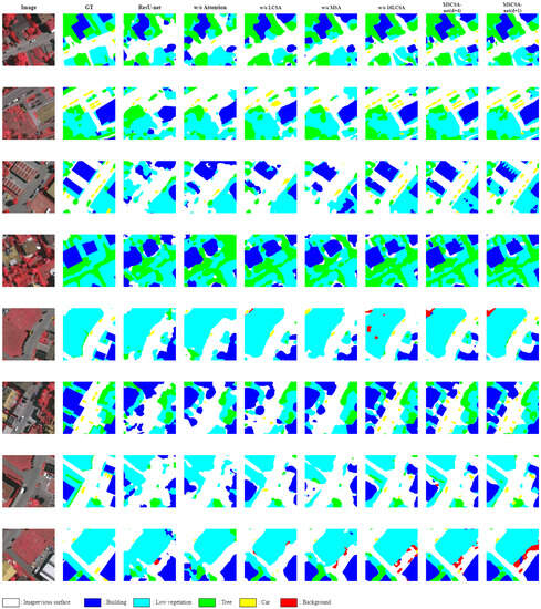
Figure 8. Visualization results with the Vaihingen dataset.

Figure 9 shows the curve maps for our training and validation with the ISPRS Vaihingen dataset, where we can see that we chose the weight with the highest validation accuracy and number of epochs to apply in the test and output the result.

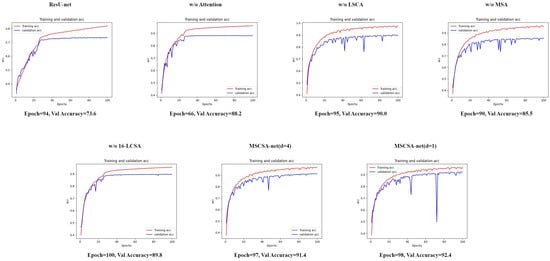
Figure 9. ISPRS Vaihingen dataset: training and validation curve maps.

Analysis of results for ISPRS Potsdam dataset. Table 2 shows the segmentation results for the test images of the Potsdam dataset. In the first row, the results were obtained from implementing ResU-Net, and these results were used as the baseline results for comparison.

Table 2. Ablation study with the Potsdam dataset. The F1-score was used as the evaluation metric for each category. The overall results were evaluated using the m-F1-score and mIoU. The bold number means the best performance among all methods.

Methods	Params (M)	Impervious Surfaces (F1)	Buildings (F1)	Low Vegetation (F1)	Trees (F1)	Cars (F1)	m-F1	mIoU
ResU-net (baseline) [16]	39.1	70.8	67.3	53.7	48.6	22.9	63.6	46.7
MSCSA-Net without attention	41.0	84.5	86.6	69.9	70.9	68.7	80.3	67.1
MSCSA-Net without LCSA	45.3	81.9	87.4	65.4	77.5	25.1	80.3	67.0
MSCSA-Net without MSA	83.3	80.3	84.4	65.4	67.2	61.0	76.7	62.2
MSCSA-Net without 16-LCSA	87.2	85.7	89.2	71.9	73.4	77.0	82.4	70.0
MSCSA-Net (d = 4)	87.4	87.0	89.1	73.3	75.2	80.8	83.2	71.2
MSCSA-Net (d = 1)	91.7	86.9	90.0	74.3	74.2	80.6	83.7	71.9

The second row shows the results for our proposed model without any of our designed attention modules (no LCSA, no MSA, no 16-LCSA). We compared the results in the first and second rows, and it can be seen that the F1-scores for the five categories (impervious surfaces, buildings, low vegetation, trees, and cars) were all much higher than ResU-Net. The m-F1-score was 80.3, higher than the ResU-Net m-F1-score (63.6), and the mIoU was 67.1, also better than ResU-Net (46.7). This means that one can just use our MSCSA-Net without attention modules and achieve much better results than ResU-Net with the Potsdam dataset.

Then, we compared our model using any two of the attention modules. The third row shows the results for our proposed model without the LCSA module. The fourth row shows the results for our proposed model without the MSA module. The fifth row shows the results for our proposed model without the 16-LCSA module. These results were also much better than the results with ResU-Net. Among these three methods, MSCSA-Net without the 16-LCSA module also had the best performance and its m-F1-score could reach 82.4 and the mIoU could reach 70.0. This demonstrates that we can only adopt two of our designed attention modules, the LCSA and MSA modules, to achieve a higher m-F1-score and mIoU.

The sixth and seventh rows show the results for our proposed model MSCSA-Net with MSA channel reduction rates of $d=4$ and $d=1$, respectively. It can be seen that MSCSA-Net (d = 4) had the second best m-F1-score (83.2) and the second best mIoU (71.2). MSCSA-Net (d = 1) had the best m-F1-score (83.7) and the best mIoU (71.9). However, MSCSA-Net (d = 4) had the best F1-scores in three categories: impervious surfaces, trees, and cars. This means that using higher channel reduction rates (d = 4) can help our model make better judgments about small objects, such as trees and cars.

We also show the visualization results for these methods with the ISPRS Potsdam dataset. As can be seen in Figure 10, our proposed MSCSA-Net (d = 4) and MSCSA-Net (d = 1) both had better segmentation results and were more similar to the ground-truth (GT) segmentation results.

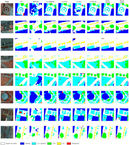
Figure 10. Visualization results for the Potsdam dataset.

Figure 11 shows the curve maps of our training and validation with the ISPRS Potsdam dataset, where we can see that we chose the weight with the highest validation accuracy and number of epochs to apply in the test and output the result.

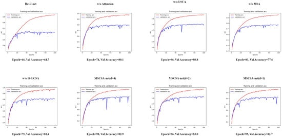
Figure 11. ISPRS Potsdam dataset: training and validation curve maps.

Ablation study of MSA channel reduction rate with the Potsdam dataset. To see the effects for different MSA channel reduction rates (d) with our proposed MSCSA-Net, we tested three channel reduction rates in the experiments on the ISPRS Potsdam dataset. Table 3 shows the segmentation results for MSA channel reduction rates d = 1, 2, and 4 with the Potsdam dataset.

Table 3. Ablation study of MSA channel reduction rate with the Potsdam dataset. The F1-score was used as the evaluation metric for each category. The overall results were evaluated using the m-F1-score and mIoU. The bold number means the best performance among all methods.

Methods	Impervious Surfaces (F1)	Buildings (F1)	Low Vegetation (F1)	Trees (F1)	Cars (F1)	m-F1	mIoU
MSCSA-Net (d = 1)	86.9	90.0	74.3	74.2	80.6	83.7	71.9
MSCSA-Net (d = 2)	86.6	88.6	73.6	75.2	80.9	83.0	71.0
MSCSA-Net (d = 4)	87.0	89.1	73.3	75.2	80.8	83.2	71.2

For the bigger objects, such as buildings and low vegetation, MSCSA-Net (d = 1) had higher F1-scores than MSCSA-Net with d = 2 and d = 4. On the other hand, both MSCSA-Net (d = 2) and MSCSA-Net (d = 4) had higher F1-scores than MSCSA-Net (d = 1) for smaller objects, such as trees and cars. We can conclude that each different MSA channel reduction rate has strengths for different sizes of objects.

4.5. Comparison of Different Methods in Terms of Segmentation Results

In this section, we compare our proposed method with some current mainstream segmentation methods using the ISPRS Vaihingen and Potsdam datasets to show the effectiveness of our method.

Comparison using ISPRS Vaihingen dataset. We tested all the compared methods with the test set of the Vaihingen dataset. The quantitative results are listed in Table 4.

Table 4. Comparison using the Vaihingen dataset. The F1-score was used as the evaluation metric for each category. The overall results were evaluated using the m-F1-score and mIoU.

Method	Impervious Surfaces (F1)	Buildings (F1)	Low Vegetation (F1)	Trees (F1)	Cars (F1)	m-F1	mIoU
ResU-net (baseline) [16]	72.1	76.0	53.9	67.3	39.4	67.1	50.5
FCN-8s [20]	71.3	71.6	63.7	65.8	44.7	77.1	63.4
SegNet [9]	75.7	88.3	62.8	77.2	37.2	77.0	64.1
CBAM [29]	78.4	80.3	67.0	68.9	52.5	81.6	69.5
RefineNet [19]	77.4	86.9	78.3	79.6	61.2	81.6	69.2
Deeplabv3+ [14]	79.4	90.0	66.9	80.1	52.6	81.5	69.5
SCAttNet [2]	80.4	${90.3}^{†}$	80.0	80.3	54.4	81.1	${70.2}^{†}$
MSCSA-Net (d = 4)	${85.4}^{†}$	90.2	72.3	${82.5}^{†}$	62.5	${82.4}^{†}$	70.1
MSCSA-Net (d = 1)	85.7	90.5	${74.2}^{†}$	82.7	${61.8}^{†}$	83.0	70.9

Bold means the best, ^† means the second best.

For the impervious surfaces category, our proposed MSCSA-Net (d = 1) had the best F1-score of 85.7. For the buildings category, our proposed MSCSA-Net (d = 1) had the best F1-score of 90.5. For the low vegetation category, SCAttNet had the best F1-score of 80.0. For the trees category, our proposed MSCSA-Net (d = 1) had the best F1-score of 82.7. For the cars category, our proposed MSCSA-Net (d = 4) had the best F1-score of 62.5.

Although MSCSA-Net (d = 1) did not have the best F1-scores for all five categories, it achieved the best overall performance. Our MSCSA-Net (d = 1) achieved m-F1 = 83.0 and mIoU = 70.9.

Comparison using the ISPRS Potsdam dataset. Our proposed method was compared with other state-of-the-art methods using the test images of the Potsdam dataset. The F1-scores, m-F1-scores, and mIoU are shown in Table 5.

Table 5. Comparison using the Potsdam dataset. The F1-score was used as the evaluation metric for each category. The overall results were evaluated using the m-F1-score and mIoU.

Method	Impervious Surfaces (F1)	Buildings (F1)	Low Vegetation (F1)	Trees (F1)	Cars (F1)	m-F1	mIoU
ResU-net (baseline) [16]	70.8	67.3	53.7	48.6	22.9	63.6	46.7
FCN-8s [20]	66.8	74.2	57.2	51.6	69.0	68.5	55.3
SegNet [9]	68.2	76.1	63.9	58.5	75.0	71.9	59.4
CBAM [29]	79.5	87.0	69.0	65.1	79.9	77.1	66.6
RefineNet [19]	77.9	79.4	69.4	65.4	78.4	75.5	64.5
Deeplabv3+ [14]	80.7	86.6	71.5	64.5	79.0	77.2	66.8
SCAttNet [2]	81.8	88.8	72.5	66.3	80.3	78.4	68.3
MSCSA-Net (d = 4)	87.0	${89.1}^{†}$	${73.3}^{†}$	75.2	80.8	${83.2}^{†}$	${71.2}^{†}$
MSCSA-Net (d = 1)	86.9	90.0	74.3	${74.2}^{†}$	${80.6}^{†}$	83.7	71.9

Bold means the best, ^† means the second best.

For the impervious surfaces category, our proposed MSCSA-Net (d = 4) had the best F1-score of 87.0. For the buildings category, our proposed MSCSA-Net (d = 1) had the best F1-score of 90.0. For the low vegetation category, our proposed MSCSA-Net (d = 1) had the best F1-score of 74.3. For the trees category, our proposed MSCSA-Net (d = 4) had the best F1-score of 75.2. For the cars category, our proposed MSCSA-Net (d = 4) had the best F1-score of 80.8.

MSCSA-Net (d = 1) did not have the best F1-scores for three categories: impervious surfaces, trees, and cars. However, it still attained the best m-F1-score (83.7) and mIoU (71.9) among all the methods compared.

5. Conclusions

In this paper, we proposed MSCSA-Net for improving semantic segmentation of remote sensing imagery. MSCSA-Net uses feature split and feature fusion from different scales twice. Specifically, three attention modules were proposed to enhance the semantic information of the features before and after fusion. The first attention module is the LCSA module, which is the attention on the experimental results and can effectively enhance the scene features The second attention module is the MSA module, which can reduce the number of parameters through the adjustment of the channel reduction rate d, which mainly helps the model perform more accurate segmentation of small objects in the RSI semantic segmentation task. The third attention module is the 16-LCSA module, which uses 16 split local features for residual SE and residual CAM operations to help the model perform more local feature enhancement on the feature map and strengthen the scene prediction of the feature map. The LCSA module with local attention is beneficial for the classification of confusing regions, while the MSA module can use different receptive fields to enhance the representation of global features.

Experimental results with two benchmark RSI datasets, the ISPRS Vaihingen and Potsdam datasets, showed that the proposed method greatly improved the representation of extracted features. The ablation study with three attention modules showed that combining the LCSA and MSA modules for our model resulted in the best accuracy. The ablation study with MSA modules showed that our model with higher channel reduction rates (e.g., d = 4) could perform better for smaller objects, such as the tree and cars categories. Our proposed model was also compared with other state-of-the-art methods using the Vaihingen and Potsdam datasets. The results showed that our MSCSA-Net (d = 1) outperformed the other methods and had the best segmentation results.

In the future, we would like to replace the backbone in MSCSA-net with other methods to analyze whether our proposed method would still be effective. As for the LCSA module, we may aim to improve this module in the direction of reducing the number of parameters to lower the running time of the model.

References

- Zheng, Z.; Zhong, Y.; Wang, J.; Ma, A. Foreground-Aware Relation Network for Geospatial Object Segmentation in High Spatial Resolution Remote Sensing Imagery. In Proceedings of the 2020 IEEE/CVF Conference on Computer Vision and Pattern Recognition (CVPR), Seattle, WA, USA, 13–19 June 2020; pp. 4095–4104. [Google Scholar] [CrossRef]
- Li, H.; Qiu, K.; Chen, L.; Mei, X.; Hong, L.; Tao, C. SCAttNet: Semantic Segmentation Network With Spatial and Channel Attention Mechanism for High-Resolution Remote Sensing Images. IEEE Geosci. Remote. Sens. Lett. 2021, 18, 905–909. [Google Scholar] [CrossRef]
- Liu, K.H.; Liu, T.J. A structure-based human facial age estimation framework under a constrained condition. IEEE Trans. Image Process. 2019, 28, 5187–5200. [Google Scholar] [CrossRef] [PubMed]
- Chen, Y.Z.; Liu, T.J.; Liu, K.H. Super-resolution of satellite images by two-dimensional rrdb and edge-enhancement generative adversarial network. In Proceedings of the ICASSP 2022–2022 IEEE International Conference on Acoustics, Speech and Signal Processing (ICASSP), Virtual, 7–13 May 2022; pp. 1825–1829. [Google Scholar]
- Liu, K.H.; Chen, T.Y.; Chen, C.S. Mvc: A dataset for view-invariant clothing retrieval and attribute prediction. In Proceedings of the 2016 ACM on International Conference on Multimedia Retrieval, New York, NY, USA, 6–9 June 2016; pp. 313–316. [Google Scholar]
- Wen, K.Y.; Liu, T.J.; Liu, K.H.; Chao, D.Y. Identifying poultry farms from satellite images with residual dense u-net. In Proceedings of the 2020 IEEE International Conference on Systems, Man, and Cybernetics (SMC), Toronto, ON, Canada, 11–14 October 2020; pp. 102–107. [Google Scholar]
- Chang, K.C.; Liu, T.J.; Liu, K.H.; Chao, D.Y. Locating waterfowl farms from satellite images with parallel residual u-net architecture. In Proceedings of the 2020 IEEE International Conference on Systems, Man, and Cybernetics (SMC), Toronto, ON, Canada, 11–14 October 2020; pp. 114–119. [Google Scholar]
- Su, Y.C.; Liu, T.J.; Liu, K.H. Wavelet Frequency Channel Attention on Remote Sensing Image Segmentation. In Proceedings of the 2022 IEEE International Conference on Consumer Electronics-Taiwan, Taipei, Taiwan, 6–8 July 2022; pp. 285–286. [Google Scholar]
- Badrinarayanan, V.; Kendall, A.; Cipolla, R. SegNet: A Deep Convolutional Encoder-Decoder Architecture for Image Segmentation. IEEE Trans. Pattern Anal. Mach. Intell. 2017, 39, 2481–2495. [Google Scholar] [CrossRef] [PubMed]
- Ronneberger, O.; Fischer, P.; Brox, T. U-Net: Convolutional Networks for Biomedical Image Segmentation. arXiv 2015, arXiv:cs.CV/1505.04597. [Google Scholar]
- Huang, L.; Dong, Q.; Wu, L.; Zhang, J.; Bian, J.; Liu, T.Y. AF _2: Adaptive Focus Framework for Aerial Imagery Segmentation. arXiv 2022, arXiv:2202.10322. [Google Scholar]
- Zheng, Z.; Zhong, Y.; Wang, J.; Ma, A.; Zhang, L. FarSeg++: Foreground-Aware Relation Network for Geospatial Object Segmentation in High Spatial Resolution Remote Sensing Imagery. IEEE Trans. Pattern Anal. Mach. Intell. 2023; 1–16, (Early Access). [Google Scholar] [CrossRef]
- Jha, A.; Bose, S.; Banerjee, B. GAF-Net: Improving the Performance of Remote Sensing Image Fusion Using Novel Global Self and Cross Attention Learning. In Proceedings of the IEEE/CVF Winter Conference on Applications of Computer Vision (WACV), Waikoloa, HI, USA, 2– 7 January 2023; pp. 6354–6363. [Google Scholar]
- Chen, L.C.; Papandreou, G.; Kokkinos, I.; Murphy, K.; Yuille, A.L. DeepLab: Semantic Image Segmentation with Deep Convolutional Nets, Atrous Convolution, and Fully Connected CRFs. IEEE Trans. Pattern Anal. Mach. Intell. 2018, 40, 834–848. [Google Scholar] [CrossRef] [PubMed]
- He, K.; Zhang, X.; Ren, S.; Sun, J. Deep Residual Learning for Image Recognition. In Proceedings of the 2016 IEEE Conference on Computer Vision and Pattern Recognition (CVPR), Las Vegas, NV, USA, 26 June–1 July 2016; pp. 770–778. [Google Scholar] [CrossRef]
- Liu, Z.; Feng, R.; Wang, L.; Zhong, Y.; Cao, L. D-Resunet: Resunet and Dilated Convolution for High Resolution Satellite Imagery Road Extraction. In Proceedings of the IGARSS 2019–2019 IEEE International Geoscience and Remote Sensing Symposium, Yokohama, Japan, 28 July–2 August 2019; pp. 3927–3930. [Google Scholar] [CrossRef]
- Zhou, Z.; Siddiquee, M.M.R.; Tajbakhsh, N.; Liang, J. UNet++: A Nested U-Net Architecture for Medical Image Segmentation. arXiv 2018, arXiv:cs.CV/1807.10165. [Google Scholar]
- Huang, H.; Lin, L.; Tong, R.; Hu, H.; Zhang, Q.; Iwamoto, Y.; Han, X.; Chen, Y.W.; Wu, J. UNet 3+: A Full-Scale Connected UNet for Medical Image Segmentation. In Proceedings of the ICASSP 2020-2020 IEEE International Conference on Acoustics, Speech and Signal Processing (ICASSP), Barcelona, Spain, 4–8 May 2020; pp. 1055–1059. [Google Scholar] [CrossRef]
- Lin, G.; Milan, A.; Shen, C.; Reid, I. RefineNet: Multi-Path Refinement Networks for High-Resolution Semantic Segmentation. In Proceedings of the 2017 IEEE Conference on Computer Vision and Pattern Recognition (CVPR), Honolulu, HI, USA, 21–26 July 2017; pp. 5168–5177. [Google Scholar] [CrossRef]
- Long, J.; Shelhamer, E.; Darrell, T. Fully convolutional networks for semantic segmentation. In Proceedings of the 2015 IEEE Conference on Computer Vision and Pattern Recognition (CVPR), Boston, MA, USA, 7–12 June 2015; pp. 3431–3440. [Google Scholar] [CrossRef]
- Sun, W.; Wang, R. Fully Convolutional Networks for Semantic Segmentation of Very High Resolution Remotely Sensed Images Combined With DSM. IEEE Geosci. Remote. Sens. Lett. 2018, 15, 474–478. [Google Scholar] [CrossRef]
- Qiao, S.; Chen, L.C.; Yuille, A. DetectoRS: Detecting Objects with Recursive Feature Pyramid and Switchable Atrous Convolution. In Proceedings of the 2021 IEEE/CVF Conference on Computer Vision and Pattern Recognition (CVPR), Nashville, TN, USA, 20–25 June 2021; pp. 10208–10219. [Google Scholar] [CrossRef]
- Jha, D.; Smedsrud, P.H.; Riegler, M.A.; Johansen, D.; Lange, T.D.; Halvorsen, P.D.; Johansen, H. ResUNet++: An Advanced Architecture for Medical Image Segmentation. In Proceedings of the 2019 IEEE International Symposium on Multimedia (ISM), San Diego, CA, USA, 9–11 December 2019; pp. 225–2255. [Google Scholar] [CrossRef]
- Kemker, R.; Luu, R.; Kanan, C. Low-Shot Learning for the Semantic Segmentation of Remote Sensing Imagery. IEEE Geosci. Remote. Sens. Lett. 2018, 56, 6214–6223. [Google Scholar] [CrossRef]
- Dai, M.; Leng, X.; Xiong, B.; Ji, K. An Efficient Water Segmentation Method for SAR Images. In Proceedings of the IGARSS 2020–2020 IEEE International Geoscience and Remote Sensing Symposium, Waikoloa, HI, USA, 26 September–2 October 2020; pp. 1129–1132. [Google Scholar] [CrossRef]
- Hu, J.; Shen, L.; Sun, G. Squeeze-and-Excitation Networks. In Proceedings of the 2018 IEEE/CVF Conference on Computer Vision and Pattern Recognition, Salt Lake City, UT, USA, 18–23 June 2018; pp. 7132–7141. [Google Scholar] [CrossRef]
- Fu, J.; Liu, J.; Tian, H.; Li, Y.; Bao, Y.; Fang, Z.; Lu, H. Dual Attention Network for Scene Segmentation. In Proceedings of the 2019 IEEE/CVF Conference on Computer Vision and Pattern Recognition (CVPR), Long Beach, CA, USA, 15–20 June 2019; pp. 3141–3149. [Google Scholar] [CrossRef]
- Lin, T.Y.; Goyal, P.; Girshick, R.; He, K.; Dollár, P. Focal Loss for Dense Object Detection. In Proceedings of the 2017 IEEE International Conference on Computer Vision (ICCV), Venice, Italy, 22–29 October 2017; pp. 2999–3007. [Google Scholar] [CrossRef]
- Woo, S.; Park, J.; Lee, J.Y.; Kweon, I.S. Cbam: Convolutional block attention module. In Proceedings of the European Conference on Computer Vision (ECCV), Munich, Germany, 8–14 September 2018; pp. 3–19. [Google Scholar]
Disclaimer/Publisher’s Note: The statements, opinions and data contained in all publications are solely those of the individual author(s) and contributor(s) and not of MDPI and/or the editor(s). MDPI and/or the editor(s) disclaim responsibility for any injury to people or property resulting from any ideas, methods, instructions or products referred to in the content. |
© 2023 by the authors. Licensee MDPI, Basel, Switzerland. This article is an open access article distributed under the terms and conditions of the Creative Commons Attribution (CC BY) license (https://creativecommons.org/licenses/by/4.0/).