Stability Prediction of Soil Slopes Based on Digital Twinning and Deep Learning

Abstract

This paper proposes a slope stability prediction model based on deep learning and digital twinning methods. To establish a reliable slope database, 30 actual slopes were collected, and 100 digital twin (DT) models were generated for each actual slope by fine-tuning the slope profiles. The safety factors of all slope samples were calculated using the Limit Equilibrium Methods (LEMs). A convolutional neural network (CNN) regression model was established, and the root mean square error (RMSE) was used as the evaluation indicator. In order to find an excellent CNN model, the K-fold (K = 10) cross-validation was used to compare the predictive effect of 1D CNN and 2D CNN on the slope safety factor. On this basis, CNN models with different network depths were compared. The results showed that the 2D CNN model with six convolutional layers had the best network prediction effect for the slope dataset. To validate the generalization ability of the model, an actual slope was input into the CNN model; its prediction result was 1.0229, and the absolute error with its real safety factor (1.0197) was 0.0032. With the slope stability prediction model proposed in this paper, the safety factor of slopes can be obtained from their geological and physical data, which greatly simplifies the calculation of the safety factor and has great engineering significance.

1. Introduction

Landslide disasters are becoming more frequent with the continued growth of the world’s population, the gradual expansion of human activities, and the continuing increase in the scale of engineering activities, coupled with other influencing factors such as global climate change. Landslides often cause traffic jams, river blockages, and disruption of civil engineering works, posing a serious threat to the safety of people’s lives and causing significant property losses. Slope stability analysis plays a key role in the prevention of slope disasters, which is an important basis for decision-making in slope design, reinforcement, and treatment as well as a long-term research topic in engineering and science.

Many methods for slope stability analysis have been developed successively in recent decades, such as engineering geological analysis methods [1], analogy methods [2], LEMs [3], numerical analysis methods [4], genetic algorithms [5,6,7], machine learning (ML) methods, etc. Among them, numerical analysis methods have been widely studied and applied [8,9,10,11,12,13,14,15,16], but they still face many problems. Especially for slopes with complex soil layers, it is usually necessary to simplify the finite element modeling. In addition, because soil layers are geometrically complex, it is difficult to mesh the slopes along the soil layers, and the modeling workload is very large. Therefore, LEMs are still the basic method of slope stability analysis, which mainly analyzes the static equilibrium of unstable soil blocks and evaluates the stability of a slope according to the Mohr-Coulomb strength criterion. The LEMs mainly include the Spencer method, the Janbu method, the Bishop method, and the unbalanced thrust method. The LEMs are easy to implement and have been tested in engineering, so they are still the most widely used methods. Chen et al. [17] proposed a simplified three-dimensional slope stability analysis method based on LEMs. Zhou et al. [18] established a rigorous limit equilibrium column method considering the intercolumn force based on six equilibrium conditions. Tang et al. [19] established the stability diagram of the homogeneous isotropic slope by using the LEMs and the strength reduction method. Song et al. [20] proposed a method to evaluate the stability of reinforced slopes based on LEMs.

However, the traditional LEMs of calculating the slope safety factor require engineers to draw slope profiles (including the geometric parameters of each soil layer) according to field exploration data and then input the slope profiles and the material parameters of the soil layers into engineering software to calculate the slope safety factor. Or, in the finite element software, the strength reduction method can be used to calculate the slope safety factor. However, the above methods require in-depth professional skills and knowledge for slope inspectors. With the development of artificial intelligence (AI), ML is becoming popular in slope stability analysis. Das et al. [21] established various artificial neural networks (ANNs) to predict the slope safety factor. Compared with support vector machines (SVM) and genetic programming (GP), ANNs are more efficient. Erzin et al. [22] used ANN and multiple regression (MR) models to predict the critical safety factor of homogeneous slopes subjected to earthquake forces. Rahul et al. [23] used ANNs to predict the safety factor of dump slopes in a coal mine. Suman et al. [24] used functional networks (FNs), multivariate adaptive regression splines (MARS), and multigene genetic programming (MGGP) to predict the safety factor of slopes and give the prediction model equation. Chakraborty et al. [25] used multiple linear regression (MLR) and ANNs to predict the stability of slopes. Bui et al. [26] intended to use optimized ANNs to design pure, cohesive slopes. Mahmoodzadeh et al. [27] predicted the safety factor of slopes by using six ML techniques.

However, most of the above studies take the internal friction angle $\phi$, the cohesion c of the slope soil, and the slope height and angle as the input parameters of each slope but do not consider the slope shape or the geometric and material parameters of each soil layer, so they are only applicable to homogeneous slopes with simple shapes. However, actual slopes are more complex and cannot be expressed simply by slope height and angle, and slopes are always composed of more soil layers. Therefore, this paper proposes a digital model that can truly reflect the authentic profiles of an actual slope and accurately predict its stability. As shown in Figure 1, it included: (1) A large number of actual slopes were collected, the DT method was used to establish the digital slope models with similar characteristics to the actual slopes, and the slope sample database was built by fine-tuning the slope profiles; (2) the LEMs were used to calculate the slope safety factor, and then the CNN model was built and trained with the slope samples. The coordinates of the slope profiles and the material parameters of the soil layers were taken as the CNN input, and the corresponding safety factor was taken as the output to train the CNN. To predict the stability of a slope, the inspectors only need to input their field exploration data into the proposed model.

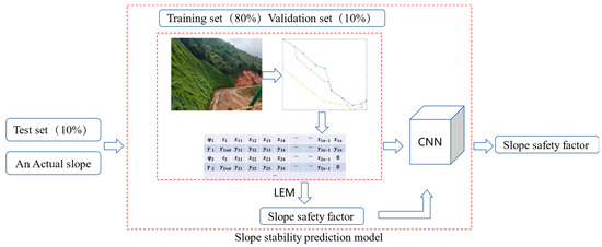
Figure 1. Slope stability prediction model.

2. Sample Collection and Digital Twins of Slopes

2.1. Slope Sample Collection

In this paper, 30 actual slopes were collected from the existing literature, and the horizontal projection length of the slopes ranged from 50 m to 3000 m. The stability state of the slopes was classified into four levels: stable, basically stable, metastable, and unstable according to the safety factor. The slope number of different types was listed in Table 1, the profiles of three slopes were shown in Figure 2, and the corresponding material parameters of their soil layers were listed in Table 2.

Table 1. Classification of slope stability state.

Slope Stability Factor	${\mathbf{F}}_{\mathbf{S}}<1.00$	$1.00\le {\mathbf{F}}_{\mathbf{S}}<1.05$	$1.05\le {\mathbf{F}}_{\mathbf{S}}<1.30$	${\mathbf{F}}_{\mathbf{S}}\ge 1.30$
Slope stability	Unstable	Metastable	Basically stable	Stable
Slope Sample	16	2	7	5

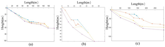
Figure 2. Slope samples: (a) Slope No.1; (b) Slope No.2; (c) Slope No.3.

Table 2. Physical and mechanical parameters of slope.

Slope Name	Soil Layer Number	c (kN/m2)	$\mathbf{\phi }$ (°)	$\mathbf{\gamma }$ (kN/m3)	${\mathbf{\gamma }}_{\mathit{sat}}(\mathbf{kN}/{\mathbf{m}}^3)$
Lion Mountain	1	0.0	25.0	18.0	18.5
	2	20.0	22.0	19.3	20.1
	3	15.5	15.0	19.5	20.2
	4	300.0	35.0	23.0	23.25
Tianshengqiao secondary gate head	1	19.6	21.8	18.1	19.0
	2	0.0	21.8	19.3	20.1
	3	29.4	20.8	18.1	19.0
	4	39.2	45.0	23.5	24.0
Yanglu Expressway K52 Slope	1	22.0	30.0	19.4	20.0
	2	30.0	27.0	20.2	21.0
	3	35.0	28.0	19.0	19.8
	4	150.0	45.0	26.5	27.0

Notes: (1) c: cohesive force; (2) $\phi :$ internal friction angle; (3) $\gamma$: natural unit weight; (4) ${\gamma }_{sat}$: saturated unit weight.

2.2. Digital Twins of Slopes

Since the number of actual slopes collected was insufficient for CNN training, as shown in Figure 3, in this paper, the DT method was used to create digital models with similar characteristics to the actual slopes, and a group of multi-size models was created by inserting some random points to fine-tune the slope profiles. Each actual slope was extended to create 100 samples. This method was able to provide sufficient CNN training samples for slope stability prediction.

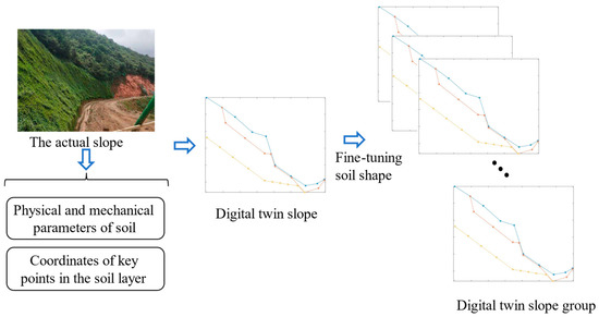
Figure 3. DT of an actual slope.

First, the outer profile line of each soil layer was represented by a polyline connected by several points, and these points that formed the original slope were called control points. The existing control points were kept unchanged, and some random points were inserted between them to fine-tune the outer shape of the slope and its soil layers and increase the number of slope samples. It should be explained here that the positive x-axis of the slope coordinate system points horizontally in the direction of the landslide, and the positive y-axis points vertically downward.

As shown in Figure 4, the number of randomly inserted points was determined by the quotient of the horizontal projection length between two connected control points divided by the corresponding threshold. According to the total length L of the horizontal projection of the slope, the following threshold was set:

$$f=\{\begin{array}{l}50\mathrm{m}L>500\mathrm{m}\\ 20\mathrm{m}500\mathrm{m}\ge L>150\mathrm{m}\\ 10\mathrm{m}150\mathrm{m}\ge L>50\mathrm{m}\\ 3\mathrm{m}L\le 50\mathrm{m}\end{array}$$

(1)

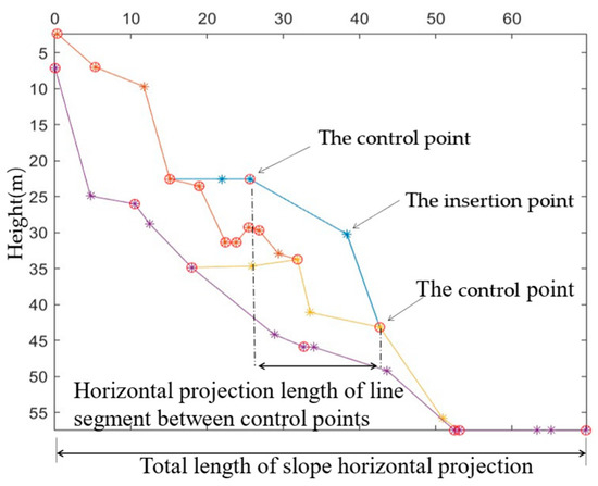
Figure 4. Insert random points to fine-tune the shape of the slope.

This method was used to fine-tune the outer contour of the slope and soil layers to generate a large number of slope models with profiles similar to the actual slope. To generate diverse samples, the vertical and horizontal coordinates of the insertion points were randomly generated within the range of the control points. In addition, it was necessary to ensure that the insertion point did not penetrate the soil layer and prevent reverse slope (Figure 5). For this reason, the following work was performed:

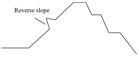
Figure 5. Reverse slope.

Between each pair of control points, the x-coordinates of the insertion points were randomly generated according to their number.

$$\mathrm{The}\mathrm{number}\mathrm{of}\mathrm{insertion}\mathrm{points}=\frac{\mathrm{the}\mathrm{horizontal}\mathrm{projection}\mathrm{length}\mathrm{between}\mathrm{the}\mathrm{control}\mathrm{points}}{\mathrm{the}\mathrm{corresponding}\mathrm{threshold}}$$

$$x_{\mathrm{P}\left(\mathrm{i}\right)}\ge x\mathrm{coordinates}\mathrm{of}\mathrm{the}\mathrm{insertion}\mathrm{points}\ge x_{\mathrm{P}\left(\mathrm{i}+1\right)}$$

As shown in Figure 6, random points were inserted from the higher control point P(i + 1) to the lower control point P(i) of the slope, and the y-coordinates of the random points were generated:

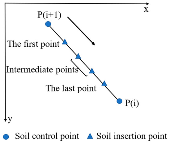
Figure 6. Insert random points between two control points.

(a) When traversing each of the slope soil layers, if there was only one insertion point within a segment, as shown in Figure 7a, the higher y-coordinate of the control point P(i + 1) and the corresponding y-coordinate of the upper soil layer of the insertion point were compared, and the maximum value (i.e., the corresponding y-coordinate of the lower soil layer of the insertion point and the y-coordinate of the control point P(i) were compared, and the minimum value (i.e., the higher point) was taken as the upper limit of the insertion point y-coordinate. If there were multiple insertion points between two control points, as in Figure 7b, the y-coordinate for the first insertion point was obtained using the above steps. For subsequent insertion points, the higher y-coordinate of the already inserted points and the y-coordinate of the upper soil layer corresponding to the insertion point were compared, and the maximum value was taken as the lower limit of the insertion point y-coordinate. The y-coordinate of the lower soil layer corresponding to the insertion point and the y-coordinate of the lower control point P(i) were also compared, and the minimum value was taken as the upper limit of the insertion point y-coordinate.

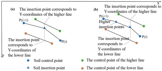
Figure 7. The insertion points of the soil layer line: (a) Only one insertion point; (b) More than one insertion point.

(b) However, in the above random point insertion process, only the upper and lower ordinates of the insertion points were considered to prevent the local soil layer from invading the lower soil layer, but the connecting line between the insertion points invading the upper layer was not considered, resulting in the situation shown in Figure 8. In this paper, self-correction methods were considered to solve such invasions.

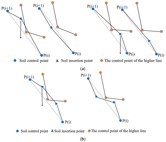
Figure 8. A self-correcting method for soil penetration. (a) The penetration point is located between the insertion point and the control point; (b) The penetration point is located between two insertion points.

For the generated soil layer, each point of the upper soil layer was checked; if the ordinate of the point of the upper soil layer was greater than that of the corresponding local layer line, it proved that there was soil layer intrusion, and the ordinate of the point was regenerated and then checked again for upper soil layer intrusion. If there was still soil layer intrusion, the above process was repeated until an insertion point without soil layer intrusion was found. If the above process was repeated more than 30 times and there was still soil intrusion, the insertion point could be moved down 5 m and then checked for soil intrusion. If there was still soil intrusion, the insertion point could be moved down another 5 m until there was no soil intrusion.

In this paper, 30 typical slopes were collected, and 100 samples were generated for each slope. A total of 3000 slope samples were generated as experimental data. This sample generation method not only maintains the rationality of the generated slopes but also greatly increases the number of samples, which meets the requirements of deep learning for big data. The partially generated slopes are shown in Table 3.

Table 3. Generated slope.

Slope Name	Actual Slope	Generated Slope
Tianshengqiao Secondary Gate Head
Yanglu Expressway K52 Slope

3. Methods

3.1. Limit Equilibrium Methods

3.1.1. Calculation of Safety Factor

In this paper, the Spencer slice method was used to calculate the safety factor. It is assumed that the soil slope slides along a certain slip plane, and the soil reaches equilibrium along this slip plane. A certain vertical soil slice was considered in the sliding soil, and its forces were shown in Figure 9:

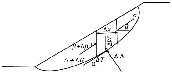
Figure 9. Force diagram of soil slice.

On the considered soil slice, ΔW is the dead weight, ΔT and ΔN are the tangential forces and the normal force at its bottom, and G is the interaction force between the slices. The differential form of the equilibrium equation was obtained by making Δ x→0, and the integral of the whole sliding surface was obtained. The force and moment balance equations of the whole sliding body [28] are shown in Equations (2) and (3), respectively:

$$G_n\left(F,\lambda \right)={{\displaystyle \int }}_a^{b}p\left(x\right)s\left(x\right)dx=0$$

(2)

$$M_n\left(F,\lambda \right)={{\displaystyle \int }}_a^{b}p\left(x\right)s\left(x\right)t\left(x\right)dx=0$$

(3)

$$p\left(x\right)=\frac{dW}{dx}sin({\phi }_e^{\prime }-\alpha )+c_e^{\prime }sec\alpha cos{\phi }_e^{\prime }$$

(4)

$$s\left(x\right)=\mathit{sec}({\phi }_e^{\prime }-\alpha +\beta )exp[-{{\displaystyle \int }}_a^{x}tan\mathit{sec}({\varphi }_e^{\prime }-\alpha +\beta )\frac{d\beta }{d\zeta }d\zeta ]$$

(5)

$$t\left(x\right)={{\displaystyle \int }}_a^x\left(sin\beta -cos\beta tan\alpha \right)exp{{\displaystyle \int }}_a^{\xi }\left[tan\left({\varphi }_e^{\prime }-\alpha +\beta \right)\frac{d\beta }{d\zeta }d\zeta \right]d\xi$$

(6)

where $\frac{dW}{dx}$ is the bulk density of the soil, $\alpha$ is the angle of inclination of the bottom of the soil slice, $c_e^{\prime }=\frac{c^{\prime }}{F}$, $\tan {\varphi }_e^{\prime }=\frac{tan{\varphi }^{\prime }}{F}$, $c^{\prime }$ is the cohesion of the soil mass, ${\varphi }^{\prime }$ is the internal friction angle of the soil, $F$ is the safety factor, and is the unknown quantity to be solved, and $\beta$ is the angle between the total force between the soil slices and the horizontal line, $tan\beta =\lambda$. Among them, $F$ and $\lambda$ are the unknowns to be solved.

The Newton-Raphson iterative method is used to solve the equilibrium equation of the above integral form to obtain $F$ and $\lambda$.

3.1.2. Optimization Method for Non-Circular Slip Surface

The slope stability analysis consists of the following two steps:

(1)

The safety factor for a slip surface in the landslide was calculated by LEMs;

(2)

For all possible slip surfaces, the above step was repeated to find the minimum safety factor and the corresponding critical slip surface.

The optimization method for the non-circular slip surface was as follows:

$$F=\left(x_1,y_1,x_2,y_2,\cdots x_n,y_n\right)$$

(7)

where $F$ is the safety factor of the non-circular slip surface calculated by LEMs, n is the number of control points of the non-circular slip surface, and $x_i,y_i$ are the coordinates of the i-th control point of the non-circular slip surface.

Since n control points correspond to 2n degrees of freedom, the non-circular slip surface optimization problem contains many degrees of freedom, and there may be many local extremum points in its independent variable space, making the task of finding the global extremum very difficult. If the slope section is complex, there may be many local extrema of the safety factor. To solve this problem, a simple and effective idea was to attempt an initial value close to the global extremum. Obviously, the closer the initial value was to the global extremum, the less likely it was to miss the global extremum. As shown in Equation (8), when searching for the minimum safety factor, the optimization of the circular slip surface involves only 3 degrees of freedom. Therefore, in this paper, the minimum safety factor of the circular sliding surface corresponding to the most dangerous sliding surface was calculated first, and the non-circular sliding surface was optimized based on it.

$$F=f\left(x_0,y_0,R\right)$$

(8)

where ($x_0,y_0)$ are the coordinates of the center of the circle and R is the radius.

In this paper, the fmincon function of the Matlab R2021a Optimization Toolbox was used to optimize the safety factor of a non-circular sliding surface with a slope. The specific steps are as follows:

(1) As shown in Figure 10, the enumeration method was used to continuously change the center coordinates ($x_0,y_0)$ and radius, and the Spencer method was used to calculate the safety factor of the circular slip surface of the slope. The minimum safety factor and the corresponding most dangerous slip surface were obtained by comparing the safety factors one by one.

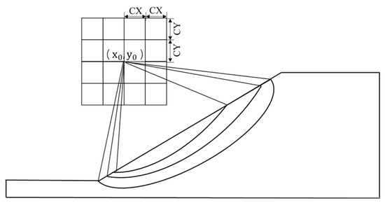
Figure 10. Enumeration method: arrange slip arcs according to different center positions and radii.

(2) As shown in Figure 11, according to the number of control points on the non-circular slip surface, the coordinates of discrete control points were uniformly selected on the most dangerous circular slip surface, and the line segments connecting these discrete points were taken as the initial slip surface in the optimization of the non-circular slip surface. The slip surface was approximately composed of (n − 1) line segments connecting n control points {($x_1,y_1$), ($x_2,y_2$),…,($x_n,y_n$)}. Points A and B are the upper and lower intersections of the slip surface and the slope, respectively; their coordinates and the horizontal coordinates of the intermediate control points are fixed, and the search variable of the non-circular slip surface composed of n control points was S = $\{y_2,$ $y_3,\dots y_{n-1}\}$. A reasonable slip surface is generally concave upward, which means that the slip surface usually needs to satisfy the following constraints [29]:

$$\mathit{tan}(85*\pi /180)>\frac{{\mathit{y}}_2{-\mathit{y}}_1}{{\mathit{x}}_2{-\mathit{x}}_1}>\frac{{\mathit{y}}_3{-\mathit{y}}_2}{{\mathit{x}}_3{-\mathit{x}}_2}>\dots >\frac{{\mathit{y}}_{\mathit{n}}{-\mathit{y}}_{\mathit{n}-1}}{{\mathit{x}}_{\mathit{n}}{-\mathit{x}}_{\mathit{n}-1}}>-\mathit{tan}(\pi /6)$$

(9)

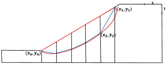
Figure 11. Optimization of non-circular slip surface.

In this paper, the safety factor of 3000 slope samples was calculated according to the above method. Figure 12 shows the optimization result of the non-circular slip surface of 2 slope samples, where the blue is the circular slip surface, the green is the initial non-circular slip surface, and the red is the optimal non-circular slip surface.

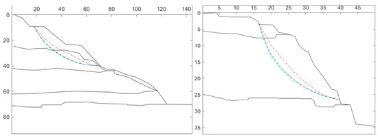
Figure 12. Optimization of non-circular slip surface of slop.

3.2. Convolutional Neural Network

3.2.1. Data Preprocessing

In this experiment, the internal friction angle $\phi$, cohesion c, natural bulk density $\gamma$, saturated bulk density ${\gamma }_{sat}$, and x and y coordinates of each soil layer of the slope were taken as the CNN input, and the corresponding safety factor was taken as the output. A 1D CNN and a 2D CNN were constructed to compare the prediction effects of the two models.

For the 2D model, as shown in Table 4, the mechanical parameters of each soil layer of the slope and the coordinates of the control points were arranged from top to bottom. Since the number of coordinate points in each soil layer was not equal and the input pattern of the neural network was a matrix, the soil layer with the largest number of line points in the slope soil layer was taken as the reference, and zeros were added at the end of the line with an insufficient number of line points. The input size of the neural network was fixed, but the size of the input matrix was not the same for different slope samples. As shown in Figure 13, the slope sample with the largest input size was taken as the reference, and zeros were added after each row and column for the samples with insufficient size.

Table 4. Preprocessing of slope input data.

${\mathit{\phi }}_1$	${\mathit{c}}_1$	${\mathit{x}}_{11}$	${\mathit{x}}_{12}$	${\mathit{x}}_{13}$	${\mathit{x}}_{14}$	…	${\mathit{x}}_{1,\mathit{n}-1}$	${\mathit{x}}_{1\mathit{n}}$
$\mathit{\gamma }$	${\gamma }_{sat}$	$y_{11}$	$y_{12}$	$y_{13}$	$y_{14}$	…	$y_{1,n-1}$	$y_{1n}$
${\mathit{\phi }}_2$	$c_2$	$x_{21}$	$x_{22}$	$x_{23}$	$x_{24}$	…	$x_{2,n-1}$	0
$\mathit{\gamma }$	${\gamma }_{sat}$	$y_{21}$	$y_{22}$	$y_{23}$	$y_{24}$	…	$y_{2,n-1}$	0
…

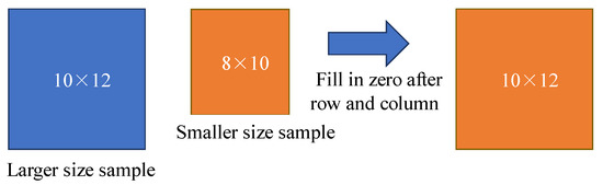
Figure 13. Normalize the dimensions of the input data.

For the 1D CNN, as shown in Figure 14, to keep the input size the same, the input data were first processed as a 2D input sample. Then, from top to bottom, the friction angle, cohesion, natural bulk density, saturated bulk density, and x and y coordinates of each soil layer of the slope were arranged in a column, and the above operations were performed on all slopes.

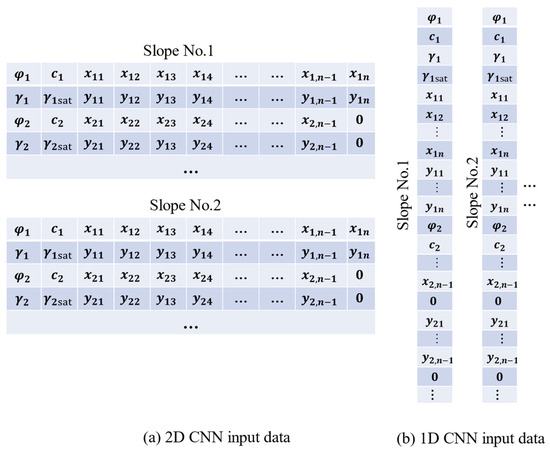
Figure 14. CNN input data.

3.2.2. CNN Regression Model

The CNN was a type of feed-forward convolutional neural network consisting of an input layer, convolutional layers, activation layers, pooling layers, normalization layers, and a fully connected layer. The convolution layer was used to extract local features from the data and was usually followed by an activation layer. Commonly used nonlinear activation functions include Sigmod, Tanh, ReLU, and Leaky ReLU. The pooling layer was used to greatly reduce the number of parameters (dimensionality reduction) and alleviate the problem of overfitting. The fully connected layer performed a nonlinear combination of the extracted features to obtain the output, which was located in the last part of the hidden layers of the CNN. The pooling layer was mainly used to reduce the dimension of the input data. Since the data volume of a single slope was much smaller than that of an image, the pooling layer was not added to the CNN in this study to prevent the loss of effective information with increasing network depth.

In this experiment, the shallow CNN model was built based on Matlab R2021a (Math Works, Inc., Natick, MA, USA). The network structure is shown in Figure 15, including an input layer and three convolutional layers with the Leaky ReLU activation function, followed by a fully connected layer and a regression layer. The parameters of the 1D CNN and 2D CNN models are shown in Table 5.

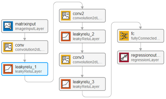
Figure 15. CNN regression mode.

Table 5. Parameters of 1D CNN and 2D CNN.

Layer		1D CNN	2D CNN
Input Layer		410 × 1	10 × 41
Conv_1	Kernel size	[2 1]	[2 2]
	Kernel num.	32	32
	Stride	[1 1]	[1 2]
	Pad	0	0
	Activation	Leaky ReLU	Leaky ReLU
Conv_2	Kernel size	[2 1]	[2 2]
	Kernel num.	64	64
	Stride	[2 1]	[2 2]
	Pad	None	None
	Activation	Leaky ReLU	Leaky ReLU
Conv_3	Kernel size	[2 1]	[2 2]
	Kernel num.	128	128
	Stride	[1 1]	[1 1]
	Pad	None	None
	Activation	Leaky ReLU	Leaky ReLU
Fully Connected Layer		1	1
Output Layer		Regression Layer	Regression Layer

The 3000 soil slope samples from Section 2.2 were divided into a training set (80%), a validation set (10%), and a test set (10%). The physical and mechanical parameters of each slope in the training set were used as input data, along with the coordinates of each soil layer, and the corresponding safety factor was used as output. The CNN-based soil slope stability prediction model was trained using this dataset. Finally, the accuracy of the CNN model was tested on the test set (10%), and an actual slope was input into the neural network to validate the universality of the CNN model.

3.3. K-Fold Cross Validation

To evaluate the generalization ability of the model, this paper adopts the K-fold cross-validation method. The commonly used K value ranges from 5 to 12, and relevant studies have confirmed that 10 is widely used [30]. This paper adopts 10-fold cross-validation, and the principle is shown in Figure 16.

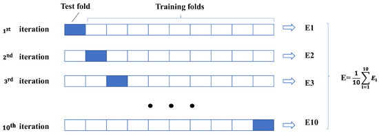
Figure 16. K-fold cross-validation.

K-fold cross-validation steps:

(1)

Step 1: The original data were randomly divided into K parts by non-repeated sampling.

(2)

Step 2: (K − 1) parts are used for model training, and the remaining 1 part is used for model testing.

(3)

Step 3: Repeat Step 2 K times to obtain the evaluation results of the K models.

(4)

Step 4: Calculate the average value of the K-fold cross-validation results as the performance evaluation of the model.

4. Results

4.1. Optimization of Non-Circular Slip Surface

The non-circular slip surfaces consisted of line segments connected by multiple control points. The safety factors were different for different numbers of control points. Based on 30 original slopes, the safety factors and optimization times of circular slip surfaces and non-circular slip surfaces with different numbers of control points are compared in this section. The comparison results are shown in Table 6 and Table 7.

Table 6. Comparisons of the safety factor of circular slip surface and non-circular slip surface with different numbers of control points.

Slope Num.	Circular Slip Surface	Safety Factors of Non-Circular Slip Surface with Different Number of Control Points
		3	4	5	6	7	8	9	10
1	0.6888	0.6813	0.6793	0.6773	0.6766	0.6723	0.6709	0.6699	0.6421
2	0.6391	0.4399	0.4373	0.4389	0.4382	0.4393	0.4373	0.4363	0.4370
3	0.1558	0.1432	0.1425	0.1420	0.1417	0.1413	0.1412	0.1411	0.1407
4	1.4556	1.4421	1.4378	1.4330	1.4288	1.4253	1.4192	1.4275	1.4316
5	0.9561	0.9230	0.9053	0.9512	0.9397	0.9243	0.9472	0.9552	0.9527
6	0.6652	0.5853	0.5821	0.5803	0.5794	0.5788	0.5785	0.5783	0.5781
7	0.4756	0.4289	0.4296	0.4287	0.4264	0.4310	0.4273	0.4265	0.4262
8	0.6033	0.5935	0.5916	0.5888	0.5865	0.5854	0.5859	0.5859	0.5854
9	1.0654	1.0379	1.0309	1.0290	1.0241	1.0241	1.0223	1.0224	1.0217
10	0.8480	0.8468	0.8409	0.8401	0.8396	0.8355	0.8336	0.8336	0.8323
11	0.5571	0.5154	0.5165	0.5136	0.5000	0.5194	0.5147	0.5127	0.5101
12	0.7304	0.6798	0.6736	0.6775	0.6567	0.5751	0.6122	0.6766	0.6495
13	0.4119	0.3688	0.3552	0.3616	0.3597	0.3596	0.3542	0.3532	0.3640
14	0.7140	0.6770	0.6725	0.6702	0.6622	0.6644	0.6622	0.6633	0.6615
15	0.4943	0.4765	0.4759	0.4704	0.4690	0.4672	0.4676	0.4611	0.4631
16	1.0615	1.0438	1.0353	1.0300	1.0261	1.0224	1.0206	1.0194	1.0166
17	1.0527	1.0513	1.0495	1.0479	1.0473	1.0466	1.0459	1.0451	1.0445
18	2.5838	2.4392	2.4345	2.4331	2.4244	2.4280	2.4234	2.4238	2.4232
19	0.9984	0.9930	0.9861	0.9793	0.9760	0.9717	0.9702	0.9688	0.9663
20	1.3076	1.1761	1.1579	1.1493	1.1691	1.1575	1.1479	1.1415	1.1355
21	1.3012	1.2856	1.2855	1.2808	1.2776	1.2801	1.2711	1.2833	1.2771
22	0.7169	0.7099	0.7067	0.6957	0.7059	0.6845	0.6946	0.6945	0.6917
23	1.4715	1.4461	1.4201	1.4191	1.4095	1.4429	1.4139	1.4366	1.4353
24	1.2645	1.1801	1.1756	1.1732	1.1713	1.1690	1.1679	1.1670	1.1647
25	2.0131	2.0129	2.0016	1.9781	1.9879	1.9621	1.9763	1.9473	1.9457
26	0.8136	0.7841	0.7832	0.7826	0.7818	0.7801	0.7800	0.7765	0.7729
27	1.0488	1.0252	1.0236	1.0224	1.0214	1.0203	1.0197	1.0191	1.0178
28	1.1915	1.1878	1.1840	1.1808	1.1791	1.1787	1.1779	1.1776	1.1771
29	1.7549	1.7476	1.7471	1.7452	1.7431	1.7414	1.7347	1.7255	1.7222
30	1.5475	1.5344	1.4971	1.4771	1.4627	1.4507	1.4440	1.4399	1.4292

Table 7. Comparisons of optimization time for different numbers of control points.

Slope Num.	Circular Slip Surface	Optimization Time of Non-Circular Slip Surface with Different Numbers of Control Points
		3	4	5	6	7	8	9	10
1	17.6	32.2	46.4	46.5	60.4	81.8	98.6	123.6	146.1
2	28.3	37.9	44.6	53.0	70.5	82.1	81.9	110.1	111.6
3	4.7	14.7	26.1	35.1	47.5	62.4	77.6	97.8	114.2
4	5.7	19.6	21.1	23.8	24.7	27.8	30.1	30.2	30.7
5	22.5	62.3	50.8	37.3	36.3	59.1	42.5	38.2	40.3
6	7.4	14.6	18.1	30.7	37.9	42.5	59.8	71.6	77.6
7	5.2	22.5	35.3	36.9	47.9	55.4	59.0	67.1	76.5
8	5.9	15.5	13.8	21.7	44.3	51.9	37.9	31.6	25.9
9	4.6	11.4	13.5	15.8	18.6	31.1	38.5	31.5	41.4
10	1.2	8.5	21.5	12.4	15.7	27.1	32.8	38.4	46.1
11	2.3	13.0	37.5	25.5	33.3	49.0	48.3	47.0	79.0
12	2.6	8.7	20.2	17.0	21.2	20.2	26.4	37.3	41.2
13	3.1	29.8	29.1	35.6	38.5	40.9	51.5	57.3	64.2
14	8.3	31.8	32.9	33.8	26.0	30.1	39.3	35.9	39.9
15	3.6	14.8	23.2	26.0	32.5	44.5	48.5	50.9	52.5
16	1.4	8.4	11.4	15.4	21.9	25.9	34.1	38.1	45.6
17	1.8	7.9	10.7	15.7	20.9	25.7	30.3	43.2	47.0
18	5.0	10.7	12.4	19.4	23.3	26.3	33.1	35.5	48.5
19	3.1	11.1	22.4	23.6	30.2	38.1	47.1	63.2	75.9
20	1.8	10.7	20.9	32.4	45.7	48.7	53.6	67.2	79.7
21	2.1	6.9	12.6	18.6	22.2	31.1	33.1	43.9	51.9
22	1.1	2.3	20.5	21.7	22.8	34.9	41.9	42.3	53.0
23	57.2	66.5	78.5	78.7	86.8	114.1	111.9	115.4	137.1
24	2.5	10.2	15.1	19.0	24.4	30.7	37.3	48.7	58.7
25	1.4	15.4	16.6	17.7	21.9	25.7	20.5	42.0	22.8
26	3.8	23.2	29.2	32.1	34.2	49.9	51.8	68.8	73.2
27	11.9	26.6	30.5	38.3	50.3	68.1	79.2	99.8	115.0
28	4.2	11.8	12.9	19.0	19.6	30.5	35.7	39.6	51.8
29	7.8	20.0	22.4	29.6	42.5	53.1	59.9	73.8	85.9
30	1.9	6.2	8.7	12.1	15.7	20.0	26.9	27.8	39.1

In comparison, it was found that for most slopes, the safety factor of a non-circular slip surface gradually decreases with the increase of the number of control points, and for very few slopes, the safety factor of a non-circular slip surface fluctuates with the increase of the number of control points. The change in the safety factor with each increase in the number of control points does not exceed 0.1. When the control points of the non-circular slip surface of the 12th slope were 6 and 7, the maximum difference in the safety factor was 0.0816. The difference between the maximum value and the minimum value of the safety factor of the noncircular slip surface was 0.1047 and 0.1052 for the 12th and 30th slopes, respectively, and the difference for other slopes was not larger than 0.1, but the optimization time greatly increases with the increase of the control points. Since the six control points can roughly reflect the shape of the slip surface of the soil slope, in this paper, the non-circular slip surface with six control points was used to calculate the safety factor of the three-thousand generated slope samples.

By comparing the minimum safety factor of the non-circular sliding surface with that of the circular sliding surface, it was found that the safety factor of the non-circular sliding surface is smaller than that of the circular sliding surface, as shown in Figure 17. Among them, the difference in the safety factor of the 2nd, 12th, 18th, 20th, 24th, and 30th slopes is 0.202, 0.155, 0.161, 0.160, 0.100, and 0.118, respectively, and the difference of the other slopes is not larger than 0.1. The slope stability states were classified according to Table 1. Except for the 9th and 17th slopes, the stability states of the slopes determined based on the safety factors of the circular slip surface and the non-circular slip surface were the same, but the calculation time of the safety factors of the non-circular slip surface was 4–50 times that of the circular slip surface. For the 9th and 17th slopes, the safety factors of the circular slip surface were 1.1080 and 1.0527, respectively, which were basically stable slopes, but the minimum safety factors of the non-circular slip surface were 1.0217 and 1.0445, respectively, which were metastable slopes. Therefore, when the safety factor was around the critical value of slope stability state division, the slope stability state divided based on the safety factor of the non-circular slip surface and the safety factor of the circular slip surface could be different, and the slope stability state divided based on the safety factor of the non-circular slip surface was safer and more conservative.

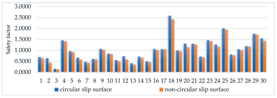
Figure 17. The safety factor of circular slip surface vs. the minimum value of safety factor of non-circular slip surface.

4.2. Slope Stability Prediction Based on CNN

4.2.1. Comparison between 1D CNN and 2D CNN

In this section, the slope sample data were pre-processed, of which 80% (2400) were used as the training set, 10% (300) as the validation set, and 10% (300) as the test set. The prediction effects of 1D CNN and 2D CNN based on the safety factors of the non-circular slip surface and circular slip surface of the slope, respectively, were compared. The same hyperparameters were used in both network models, and the specific parameters are shown in Table 8. The RMSE was used as the evaluation indicator. The results of the 10-fold cross-validation of the two CNN models are shown in Table 9.

Table 8. Hyperparameter settings.

Parameter	Value
Solver	Adam
Max Epoch	40
minibatch size	20
Initial Learning Rate	0.001
Validation Frequency	50
Learn Rate Drop Period	10
Learn Rate Drop Factor	0.3

Table 9. RMSE of the model under 10-fold cross-validation.

	Model	Non-Circular Slip Surfaces		Circular Slip Surfaces
Iteration		1D	2D	1D	2D
1st		0.0770	0.0770	0.0799	0.0782
2nd		0.0776	0.0770	0.0759	0.0777
3rd		0.0742	0.0742	0.0760	0.0767
4th		0.0729	0.0725	0.0733	0.0716
5th		0.0718	0.0686	0.0718	0.0668
6th		0.0778	0.0779	0.0769	0.0771
7th		0.0852	0.0826	0.0803	0.0768
8th		0.0758	0.0727	0.0760	0.0719
9th		0.0783	0.0783	0.0836	0.0797
10th		0.0807	0.0785	0.0850	0.0843
Average		0.0771	0.0759	0.0779	0.0761

By comparing the average value of the RMSE of the 10-fold cross-validation of each model, it was found that for the 1D CNN model and the 2D CNN model, the RMSE of the prediction model based on the non-circular slip surfaces was slightly lower than that based on the circular slip surface, while for the two slip surfaces, the RMSE of the 2D CNN was slightly lower than that of the 1D CNN, which may be due to the input of the 2D CNN in the form of a matrix. Every two rows of data from the 2D input samples correspond to the mechanical parameters and coordinates of one soil layer. The size of the 2D CNN convolution kernel was 2 × 2. In the convolution process, the independence of information for each soil layer and the correlation between soil layers are maintained. Therefore, the following tests adopt the 2D CNN model based on a non-circular slip surface.

4.2.2. Comparison of CNN Models with Different Depths

The CNN was composed of multiple convolutional layers, and the predictive performance of the network model composed of different numbers of convolutional layers was different. To find the most suitable network model for the experimental dataset, six different depth network models were compared. As shown in Table 10, the network structure of Model 1 ~ Model 5 was similar, and only one convolutional layer was increased in turn. As shown in Figure 18, Model 6 was a depth residual network. The hyperparameters of all the network models are shown in Table 8.

Table 10. Network structure.

Model	Layer	Type	Kernel Num.	Kernel Size	Stride	Pad	Activation
1	1 2 3 4	Input $\mathrm{Conv}\_1^{a)}$ ${\mathrm{FC}}^{b)}$ Regression	— 32 — —	— 2 × 2 — —	— [1,1] — —	— 0 — —	— Leaky ReLU — —
2	1 2 3 4 5	Input $\mathrm{Conv}\_1^{a)}$ $\mathrm{Conv}\_2^{a)}$ ${\mathrm{FC}}^{b)}$ Regression	— 32 64 — —	— 2 × 2 2 × 2 — —	— [1,1] [2,2] — —	— 0 0 — —	— Leaky ReLU Leaky ReLU — —
3	1 2 3 4 5 6	Input $\mathrm{Conv}\_1^{a)}$ $\mathrm{Conv}\_2^{a)}$ $\mathrm{Conv}\_3^{a)}$ ${\mathrm{FC}}^{b)}$ Regression	— 32 64 128 — —	— 2 × 2 2 × 2 2 × 2 — —	— [1,1] [2,2] [1,1] — —	— 0 0 0 — —	— Leaky ReLU Leaky ReLU Leaky ReLU — —
4	1 2 3 4 5 6 7	Input $\mathrm{Conv}\_1^{a)}$ $\mathrm{Conv}\_2^{a)}$ $\mathrm{Conv}\_3^{a)}$ $\mathrm{Conv}\_4^{a)}$ ${\mathrm{FC}}^{b)}$ Regression	— 32 64 128 256 — —	— 2 × 2 2 × 2 2 × 2 2 × 2 — —	— [1,1] [2,2] [1,1] [1,1] — —	— 0 0 0 0 — —	— Leaky ReLU Leaky ReLU Leaky ReLU Leaky ReLU — —
5	1 2 3 4 5 6 7 8	Input $\mathrm{Conv}\_1^{a)}$ $\mathrm{Conv}\_2^{a)}$ $\mathrm{Conv}\_3^{a)}$ $\mathrm{Conv}\_4^{a)}$ $\mathrm{Conv}\_5^{a)}$ ${\mathrm{FC}}^{b)}$ Regression	— 32 64 128 256 512 — —	— 2 × 2 2 × 2 2 × 2 2 ×2 2 × 2 — —	— [1,1] [2,2] [1,1] [1,1] [1,1] — —	— 0 0 0 0 0 — —	— Leaky ReLU Leaky ReLU Leaky ReLU Leaky ReLU Leaky ReLU — —
6	1 2 3 4 5 6 7 8 9	Input $\mathrm{Conv}\_1^{a)}$ $\mathrm{Conv}\_2^{a)}$ $\mathrm{Conv}\_3^{a)}$ $\mathrm{Conv}\_4^{a)}$ $\mathrm{Conv}\_5^{a)}$ $\mathrm{Conv}\_6^{a)}$ ${\mathrm{FC}}^{b)}$ Regression	— 32 64 128 256 256 512 — —	— 2 × 2 2 × 2 2 × 2 2 × 2 2 × 2 2 × 2 — —	— [1,1] [2,2] [1,1] [1,1] [1,1] [1,1] — —	— 0 0 0 0 0 0 — —	— Leaky ReLU Leaky ReLU Leaky ReLU Leaky ReLU Leaky ReLU Leaky ReLU — —
7	1 2 3 4 5 6 7 8 9 10	Input $\mathrm{Conv}\_1^{a)}$ $\mathrm{Conv}\_2^{a)}$ $\mathrm{Conv}\_3^{a)}$ $\mathrm{Conv}\_4^{a)}$ $\mathrm{Conv}\_5^{a)}$ $\mathrm{Conv}\_6{}^{a)}$ $\mathrm{Conv}\_7^{a)}$ ${\mathrm{FC}}^{b)}$ Regression	— 32 64 128 256 256 512 512 — —	— 2 × 2 2 × 2 2 ×2 2 × 2 2 × 2 2 × 2 2 × 2 — —	— [1,1] [1,1] [1,1] [1,1] [1,1] [1,1] [1,1] — —	— 0 0 0 0 0 0 0 — —	— Leaky ReLU Leaky ReLU Leaky ReLU Leaky ReLU Leaky ReLU Leaky ReLU Leaky ReLU — —

Notes: a) Conv_#: Convolutional layer; b) FC: fully connected layer.

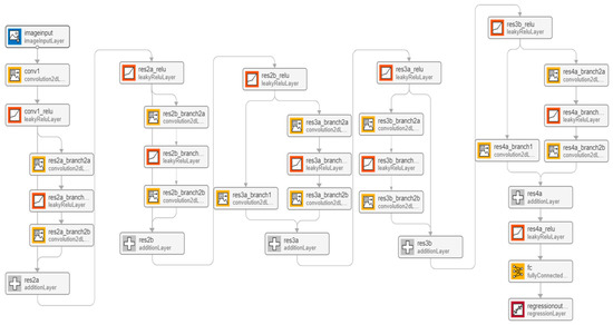
Figure 18. Residual network structure.

The RMSE of network models with different depths is shown in Figure 19. As the number of network convolutional layers increased from three to six, the RMSE of the network model became smaller and smaller, and the prediction effect became better and better. However, when the number of convolutional layers was seven, the RMSE of the network model was significantly larger than that of the network model (Model 4) with six convolutional layers. The RMSE of the residual depth network model was the largest at 0.0696. Obviously, it was not the case that the deeper the number of network layers, the better the network prediction effect. Especially when the sample data volume is small, as the number of network layers increases, less effective information can be extracted for the deeper convolutional layer. Therefore, for this experimental dataset, the 2D CNN model with six convolutional layers has the best performance with an RMSE of 0.0666. The comparative results of the network hyperparameter optimization are shown in Appendix A.

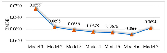
Figure 19. RMSE of CNN models with different depths.

4.2.3. Prediction Results

In this paper, a six-layer 2D CNN model is built. The network structure is shown in Model 4 in Table 7. The network solver adopts Adam, the initial learning rate is 0.001, and 300 (10%) verification sets are taken as the test set. The prediction performance of the model is shown in Figure 20.

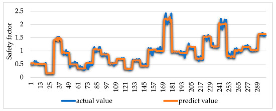
Figure 20. Model prediction results.

In order to verify the generalization ability of the model, this paper collects a typical landslide case from the existing literature. The landslide is located in Qingning Township, Daxian County, Sichuan Province. The slope shape is shown in the figure, and the physical parameters of the soil are listed in Table 11. The coordinate information and the physical and mechanical parameters of the soil layer are arranged as shown in Table 3 and input into the trained network model. The actual slope safety factor is 1.0197, the model prediction result is 1.0229, and the absolute error is 0.0032, which verifies the applicability of the model.

Table 11. Qingning Town landslide, Daxian County, Sichuan Province.

Slope Name	The Slope Shape	Soil Layer	c	$\mathit{\phi }$	$\mathit{\gamma }$	${\mathit{\gamma }}_{\mathit{s}\mathit{a}\mathit{t}}$
Qingning Town landslide, Daxian County, Sichuan Province		Quaternary sediment	34	27	18.8	24
		Strongly weathered sandstone	220.8	44	22.5	27.4
		Weakly weathered mudstone	120.7	32	24	26
		Weakly weathered sandstone	350.5	52	25.5	28.8

5. Conclusions

In this paper, the DT method was used to build a slope stability prediction model based on big data and deep learning. Initially, the sample database of the slope was established by using the sample generation method, and the optimized safety factor of the non-circular slip surface was compared with the safety factor of the circular slip surface. Secondly, the CNN regression model is established, and the predictive effects of 1D and 2D network models and different depth network models are compared, respectively. The following conclusions are drawn:

• The DT slope models generated based on the LEMs greatly expand the slope sample dataset while maintaining the rationality of the slope samples, thus providing robust training samples for the big data-based deep learning method to predict slope stability.
• Based on the circular slip surface, the safety factor of the non-circular slip surface is optimized, and the safety factor is smaller than that of the circular slip surface. The minimum safety factor of the non-circular slip surface decreases slightly as the number of control points on the slip surface increases, but the computation time increases significantly. The RMSE of the prediction model based on the non-circular slip surface is slightly lower than that based on the circular slip surface.
• For this experimental dataset, the RMSE of 2D CNN was slightly lower than that of 1D CNN. The RSME of CNN first decreases and then increases as the number of network layers increases.
• The prediction model of slope safety factor based on CNN had strong generalization ability, and the prediction error was within an acceptable range, providing a method for rapid detection of slope stability.

In this paper, the DT slope stability prediction model based on CNN is built. The inspector only needs to input the exploration data into the slope stability prediction model to obtain the safety factor of the slope. The procedure is simple, does not require strong professional knowledge, and has great engineering application value. However, the input data may be redundant. In future studies, sensitivity analysis will be carried out, and pruning and other methods will be considered for clipping input data from slopes. In addition, this study only considers 2D slopes, and in a later stage, a 3D slope sample database can be constructed by combining finite element analysis to achieve 3D slope stability prediction. Finally, this study only focuses on the study of slope stability prediction methods based on CNNs. In the future, a user-oriented intelligent detection platform can be developed to promote the real implementation of this research result in slope engineering practice.

References

- Su, M.H.; Ma, X.D.; Li, X. Analysis of Engineering Geological Mechanics on the Jiasikou Debris Flow. Appl. Mech. Mater. 2013, 385–386, 404–407. [Google Scholar] [CrossRef]
- Zhou, H.Q.; Liu, D.S.; Chen, Z.H. Analogy Method and It’s Application in the Landslide Control Engineering. Chin. J. Undergr. Space Eng. 2008, 4, 1057–1060. [Google Scholar]
- Duncan, J.M.; Wright, S.G. Soil Strength and Slope Stability; Wiley: Chichester, UK, 2005. [Google Scholar]
- Yang, G.H.; Zhong, Z.H.; Zhang, Y.C.; Li, D.J. Slope stability analysis by local strength reduction method. Rock Soil Mech. 2010, 31, 53–58. [Google Scholar]
- Wang, H.; Moayedi, H.; Foong, L.K. Genetic algorithm hybridized with multilayer perceptron to have an economical slope stability design. Eng. Comput. 2021, 37, 3067–3078. [Google Scholar] [CrossRef]
- Zheng, Y.; Chen, C.X.; Meng, F.; Zhang, H.N.; Xia, K.Z.; Chen, X.B. Assessing the Stability of Rock Slopes with Respect to Block-Flexure Toppling Failure Using a Force-Transfer Model and Genetic Algorithm. Rock Mech. Rock Eng. 2020, 53, 3433–3445. [Google Scholar] [CrossRef]
- Zhou, X.P.; Huang, X.C.; Zhao, X.F. Optimization of the Critical Slip Surface of Three-Dimensional Slope by Using an Improved Genetic Algorithm. Int. J. Geomech. 2020, 20, 04020120. [Google Scholar] [CrossRef]
- Dyson, A.P.; Tolooiyan, A. Comparative Approaches to Probabilistic Finite Element Methods for Slope Stability Analysis. Simul. Model. Pract. Theory 2020, 100, 102061. [Google Scholar] [CrossRef]
- Li, Z.; Hu, Z.; Zhang, X.Y.; Du, S.G.; Guo, Y.K.; Wang, J.X. Reliability analysis of a rock slope based on plastic limit analysis theory with multiple failure modes. Comput. Geotech. 2019, 110, 132–147. [Google Scholar] [CrossRef]
- Lim, K.; Li, A.J.; Schmid, A.; Lyamin, A.V. Slope-Stability Assessments Using Finite-Element Limit-Analysis Methods. Int. J. Geomech. 2017, 17, 06016017. [Google Scholar] [CrossRef]
- Liu, S.Y.; Su, Z.N.; Li, M.; Shao, L.T. Slope stability analysis using elastic finite element stress fields. Eng. Geol. 2020, 273, 105673. [Google Scholar] [CrossRef]
- Oberhollenzer, S.; Tschuchnigg, F.; Schweiger, H.F. Finite element analyses of slope stability problems using non-associated plasticity. J. Rock Mech. Geotech. Eng. 2018, 10, 1091–1101. [Google Scholar] [CrossRef]
- Rawat, S.; Gupta, A.K. Analysis of a Nailed Soil Slope Using Limit Equilibrium and Finite Element Methods. Int. J. Geosynth. Ground Eng. 2016, 2, 34. [Google Scholar] [CrossRef]
- Xiao, T.; Li, D.Q.; Cao, Z.J.; Au, S.K.; Phoon, K.K. Three-dimensional slope reliability and risk assessment using auxiliary random finite element method. Comput. Geotech. 2016, 79, 146–158. [Google Scholar] [CrossRef]
- Yu, M.D. Analysis on stability of mountain mass and numerical calculation of landslide resistance based on strength reduction method. Arab. J. Geosci. 2020, 13, 617. [Google Scholar] [CrossRef]
- Zhang, T.W.; Cai, Q.X.; Han, L.; Shu, J.S.; Zhou, W. 3D stability analysis method of concave slope based on the Bishop method. Int. J. Min. Sci. Technol. 2017, 27, 365–370. [Google Scholar] [CrossRef]
- Chen, Z.Y.; Mi, H.L.; Zhang, F.M.; Wang, X.G. A simplified method for 3D slope stability analysis. Can. Geotech. J. 2003, 40, 675–683. [Google Scholar] [CrossRef]
- Zhou, X.P.; Cheng, H. Analysis of stability of three-dimensional slopes using the rigorous limit equilibrium method. Eng. Geol. 2013, 160, 21–33. [Google Scholar] [CrossRef]
- Tang, G.P.; Zhao, L.H.; Li, L.; Yang, F. Stability charts of slopes under typical conditions developed by upper bound limit analysis. Comput. Geotech. 2015, 65, 233–240. [Google Scholar] [CrossRef]
- Song, F.; Chen, R.Y.; Ma, L.Q.; Cao, G.R. A new method for the stability analysis of geosynthetic-reinforced slopes. J. Mt. Sci. 2016, 13, 2069–2078. [Google Scholar] [CrossRef]
- Das, S.K.; Biswal, R.K.; Sivakugan, N.; Das, B. Classification of slopes and prediction of factor of safety using differential evolution neural networks. Environ. Earth Sci. 2011, 64, 201–210. [Google Scholar] [CrossRef]
- Erzin, Y.; Cetin, T. The prediction of the critical factor of safety of homogeneous finite slopes subjected to earthquake forces using neural networks and multiple regressions. Geomech. Eng. 2014, 6, 1–15. [Google Scholar] [CrossRef]
- Rahul Khandelwal, M.; Rai, R.; Shrivastva, B.K. Evaluation of dump slope stability of a coal mine using artificial neural network. Geomech. Geophys. Geo-Energy Geo-Resour. 2015, 1, 69–77. [Google Scholar] [CrossRef]
- Suman, S.; Khan, S.Z.; Das, S.K.; Chand, S.K. Slope stability analysis using artificial intelligence techniques. Nat. Hazards 2016, 84, 727–748. [Google Scholar] [CrossRef]
- Chakraborty, A.; Goswami, D. Prediction of slope stability using multiple linear regression (MLR) and artificial neural network (ANN). Arab. J. Geosci. 2017, 10, 385. [Google Scholar] [CrossRef]
- Bui, X.N.; Muazu, M.A.; Nguyen, H. Optimizing Levenberg-Marquardt backpropagation technique in predicting factor of safety of slopes after two-dimensional OptumG2 analysis. Eng. Comput. 2020, 36, 941–952. [Google Scholar] [CrossRef]
- Mahmoodzadeh, A.; Mohammadi, M.; Ali, H.F.H.; Ibrahim, H.H.; Abdulhamid, S.N.; Nejati, H.R. Prediction of safety factors for slope stability: Comparison of machine learning techniques. Nat. Hazards 2022, 111, 1771–1799. [Google Scholar] [CrossRef]
- Chen, Z.Y.; Morgenstern, N.R. Extensions to the generalized method of slices for stability analysis. Can. Geotech. J. 2011, 20, 104–119. [Google Scholar] [CrossRef]
- Bai, T.; Qiu, T.; Huang, X.M.; Li, C. Locating Global Critical Slip Surface Using the Morgenstern-Price Method and Optimization Technique. Int. J. Geomech. 2014, 14, 319–325. [Google Scholar] [CrossRef]
- Zhang, Y.L.; Yang, Y.H. Cross-validation for selecting a model selection procedure. J. Econom. 2015, 187, 95–112. [Google Scholar] [CrossRef]
Disclaimer/Publisher’s Note: The statements, opinions and data contained in all publications are solely those of the individual author(s) and contributor(s) and not of MDPI and/or the editor(s). MDPI and/or the editor(s) disclaim responsibility for any injury to people or property resulting from any ideas, methods, instructions or products referred to in the content. |
© 2023 by the authors. Licensee MDPI, Basel, Switzerland. This article is an open access article distributed under the terms and conditions of the Creative Commons Attribution (CC BY) license (https://creativecommons.org/licenses/by/4.0/).