5.1. Dynamic Simulation
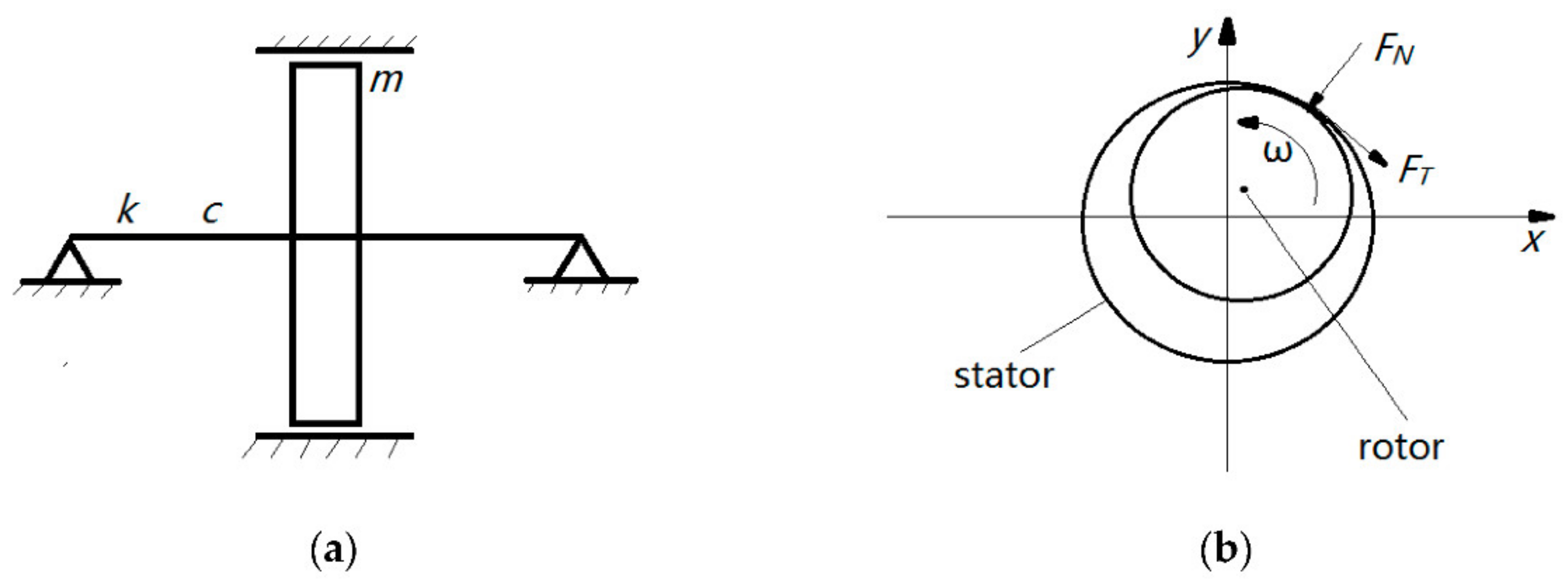
The rub-impact model discussed is a Jeffcott rotor system, as shown in
Figure 7.
The system can be described by the following equations:
in which
is the mass of the rotor system, the gravity of the rotor is
,
is the damping coefficient,
is the stiffness coefficient,
is the lateral displacement,
is the vertical displacement,
is the imbalance,
is the rotation speed,
and
are the rub-impact forces. The rub-impact forces are shown in the following equation
in which
is the radial displacement of the disk center,
is the clearance between the rotor and the stator,
is the contacting stiffness for the stator,
is the friction coefficient and the Heaviside function
is defined as
The parameters in the above equations are shown in
Table 2.
Using the fourth order Runge–Kutta method to solve for . The second derivative of , which is , using numerical method can be solved. Additionally, the step size of the numerical derivative is .
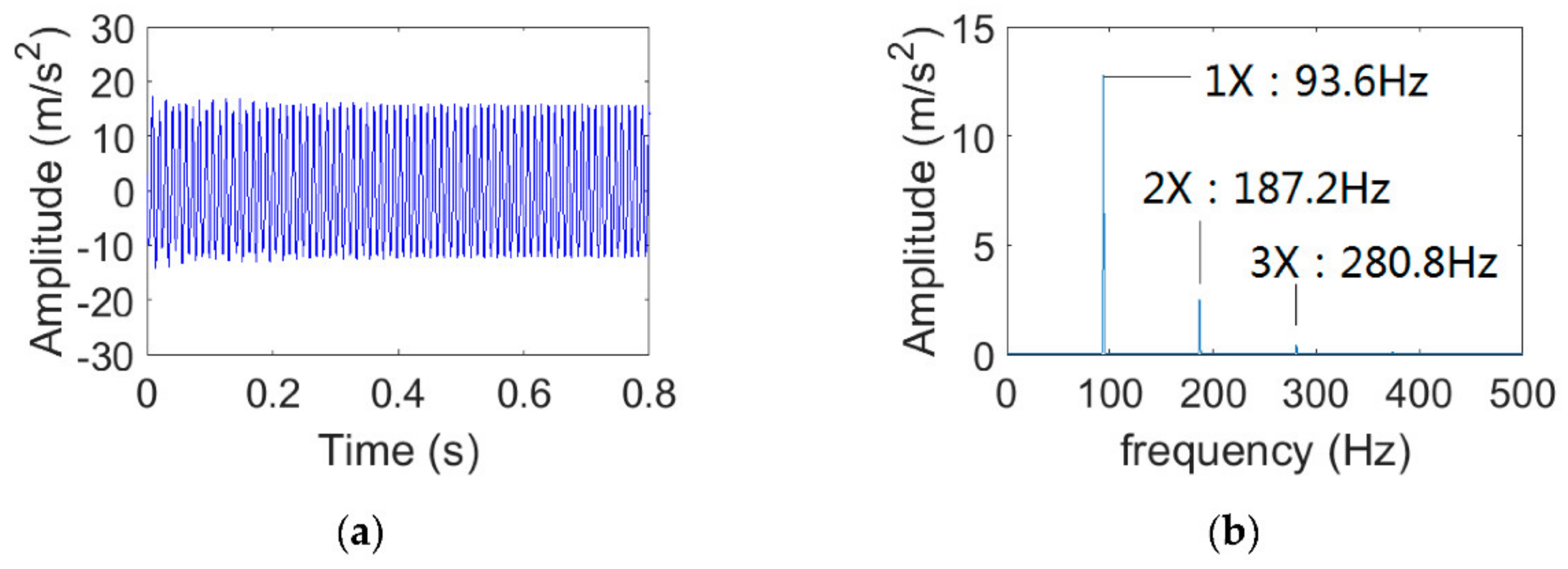
The waveform and FFT of
is revealed in
Figure 8, and
is set to 5616 r/min. It is illustrated that the amplitudes of 1× and 2× are relatively high, and the amplitude of 3× is lower, as revealed in
Figure 8b.
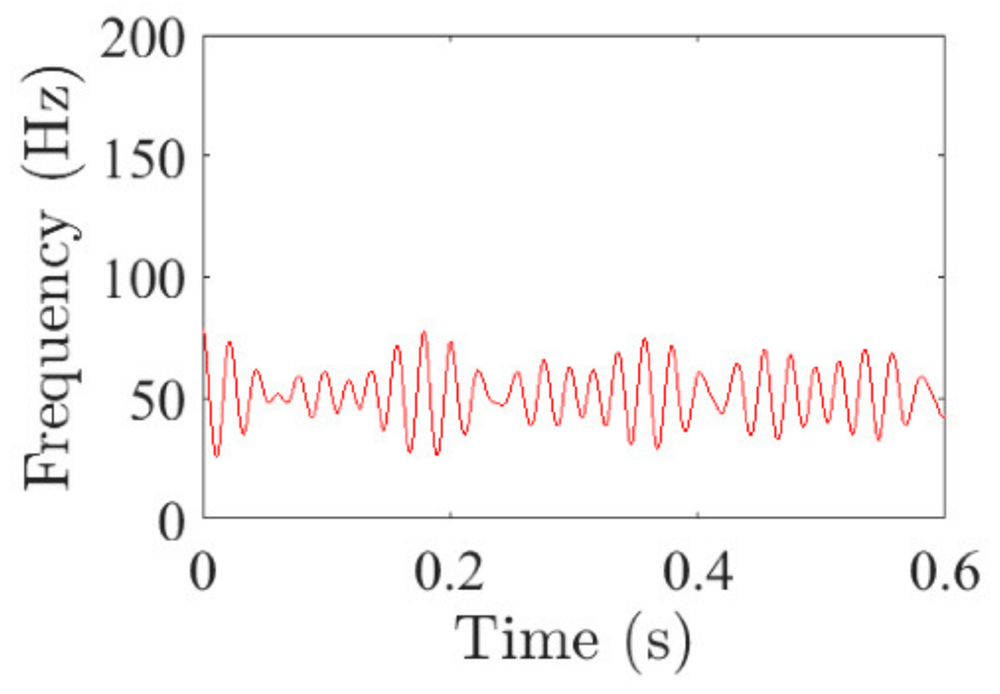
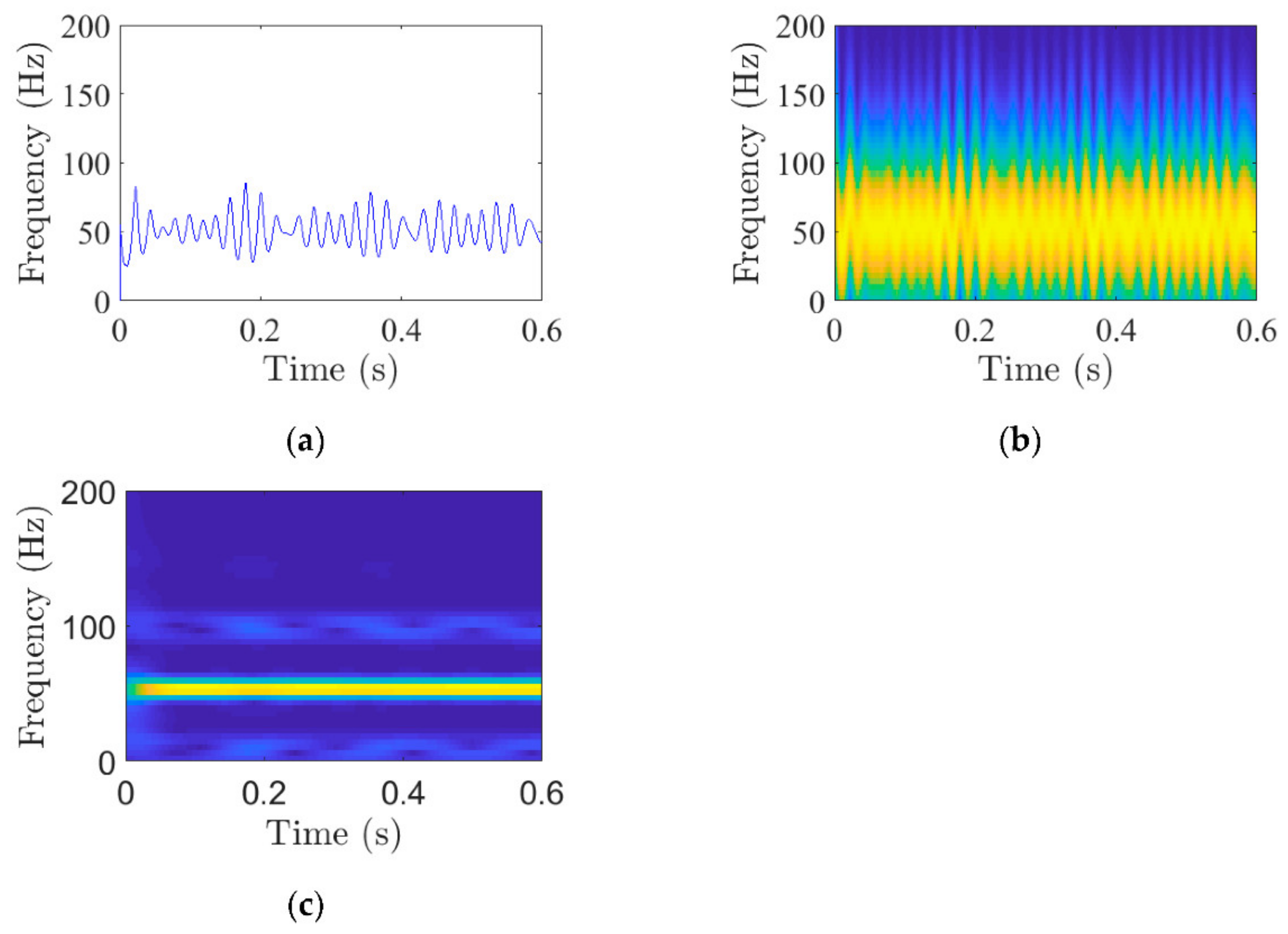
The Hilbert spectrum of
is shown in
Figure 9.
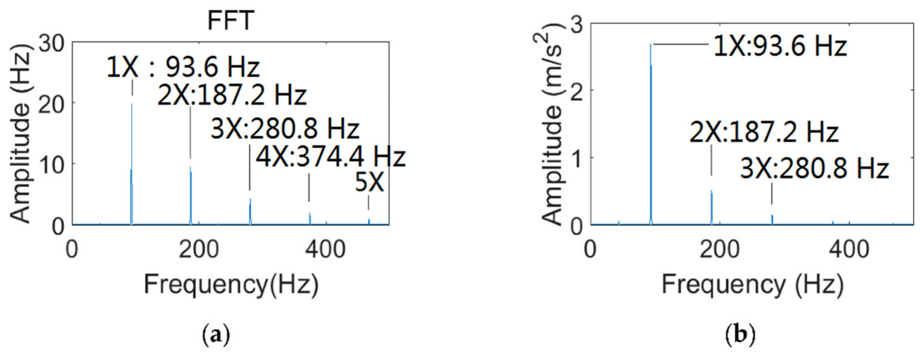
FFT is applied to the IF of 1×, and the FFT of the IF is revealed in
Figure 10a. We can see that the main fluctuating frequencies of the IF of 1× are 468.0 Hz, 374.4 Hz, 280.8 Hz, 187.2 Hz, and 93.6 Hz. Additionally, 468.0 Hz is five-times the rotation frequency, 374.4 Hz is four-times the rotation frequency, 280.8 Hz is three-times the rotation frequency, 187.2 Hz is two-times the rotation frequency, 93.6 Hz is the rotation frequency. The envelope spectrum for 1× is revealed in
Figure 10b. The main fluctuating frequencies of the envelope of 1× are 280.8 Hz, 1187.2 Hz and 93.6 Hz. Additionally, 280.8 Hz is three-times the rotation frequency, 187.2 Hz is two-times the rotation frequency, 93.6 Hz is the rotation frequency.
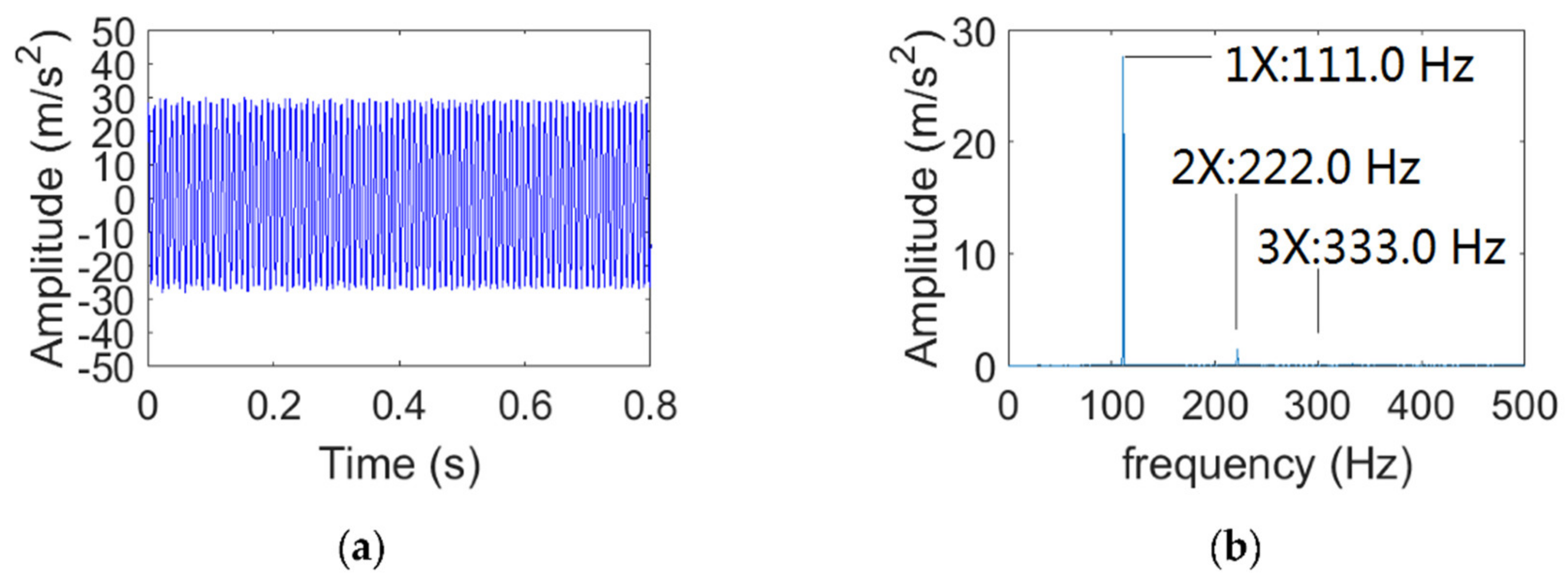
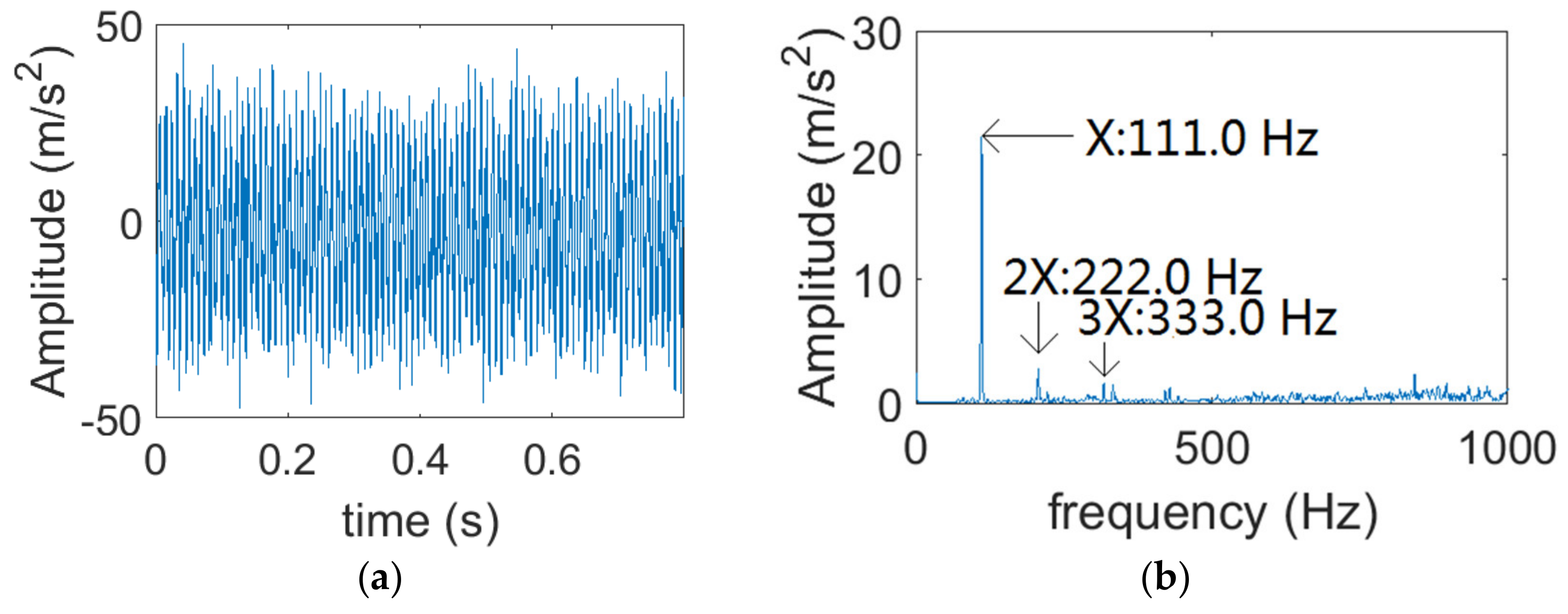
The waveform and FFT of
is revealed in
Figure 11, and
is set to 6660 r/min. It is illustrated that the amplitude of 1× is relatively high, and the amplitudes of 2× and 3× are lower, as revealed in
Figure 11b.
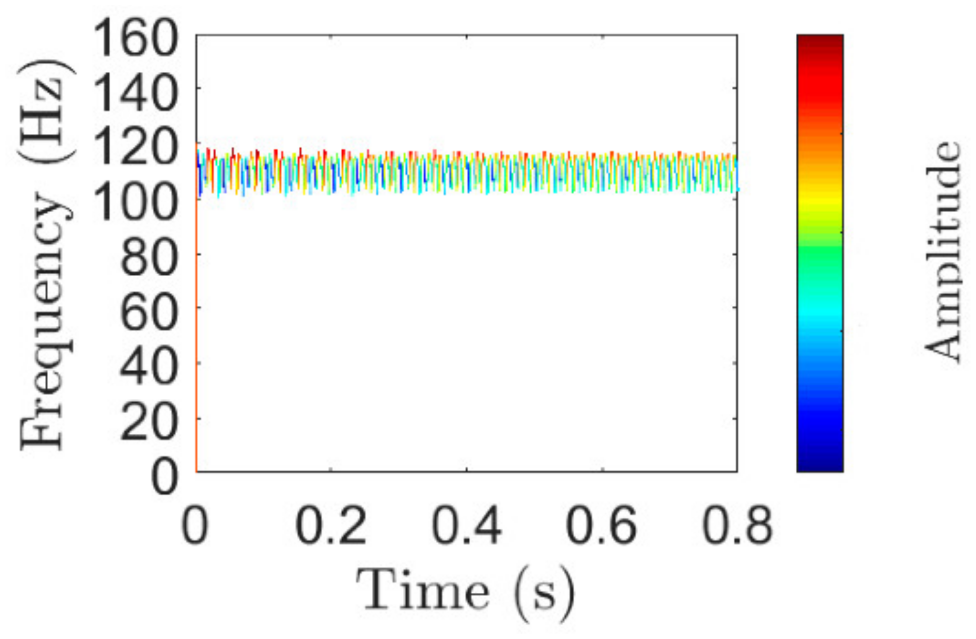
The Hilbert spectrum of
is shown in
Figure 12.
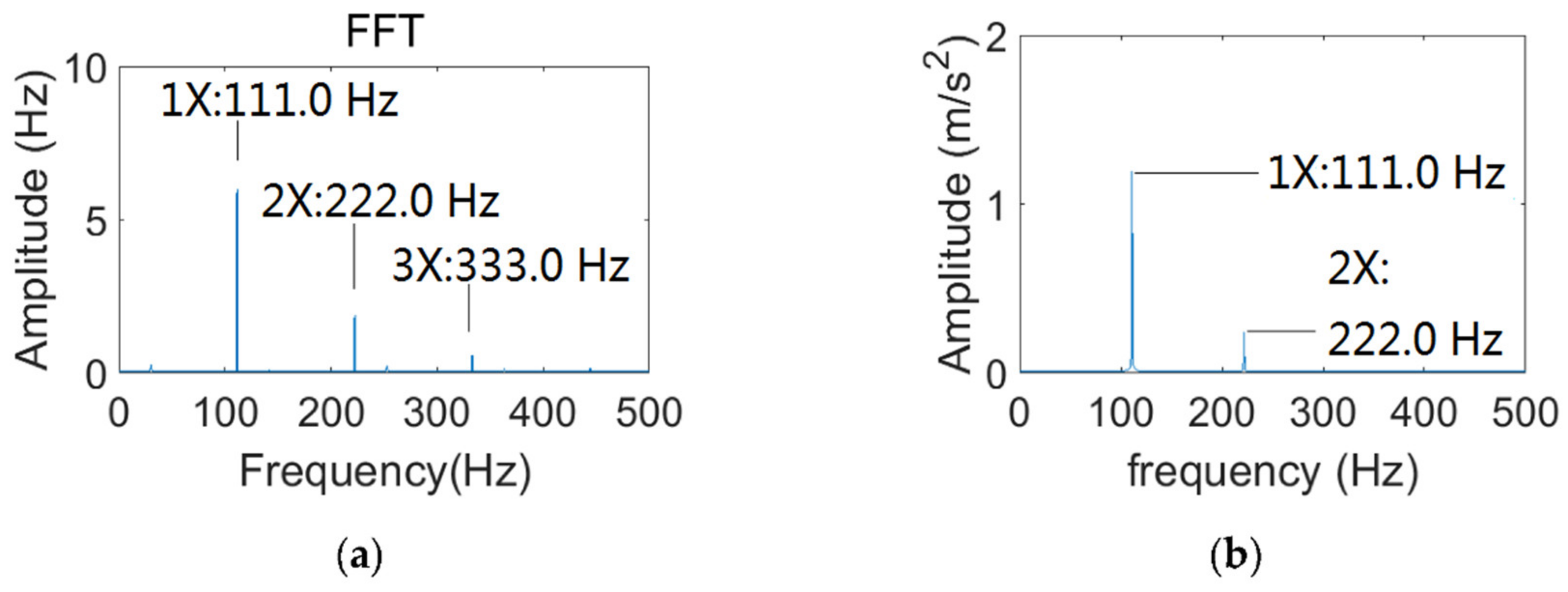
The FFT of the IF and the envelope spectrum for 1× are shown in
Figure 13. FFT is applied to the IF of 1×, and the FFT of the IF is revealed in
Figure 13a We can see that the main fluctuating frequencies of the IF of 1× are 333.0 Hz, 222.0 Hz, and 111.0 Hz. Additionally, 333.0 Hz is three-times the rotation frequency, 222.0 Hz is two-times the rotation frequency, 111.0 Hz is the rotation frequency. The envelope spectrum for 1× is revealed in
Figure 13b. The main fluctuating frequencies of the envelope of 1× are 222.0 Hz and 111.0 Hz. Additionally, 222.0 Hz is two-times the rotation frequency, 111.0 Hz is the rotation frequency.
5.2. Application to Vibration Signals of Aeroengine
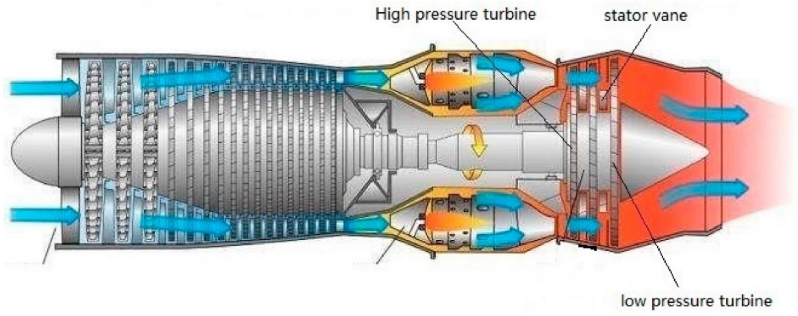
The structure sketch of the aeroengine is revealed in
Figure 14. The rotation speed of the low-pressure turbine is approximately 5616 r/min (93.6 Hz), and the rotation speed of the high pressure turbine is approximately 10,445 r/min (174.1 Hz). A charge output accelerometer was used to measure the vibration acceleration, which was installed on the outer surface of aeroengine casing. There existed rubbing between the low-pressure turbine and the stator vane.
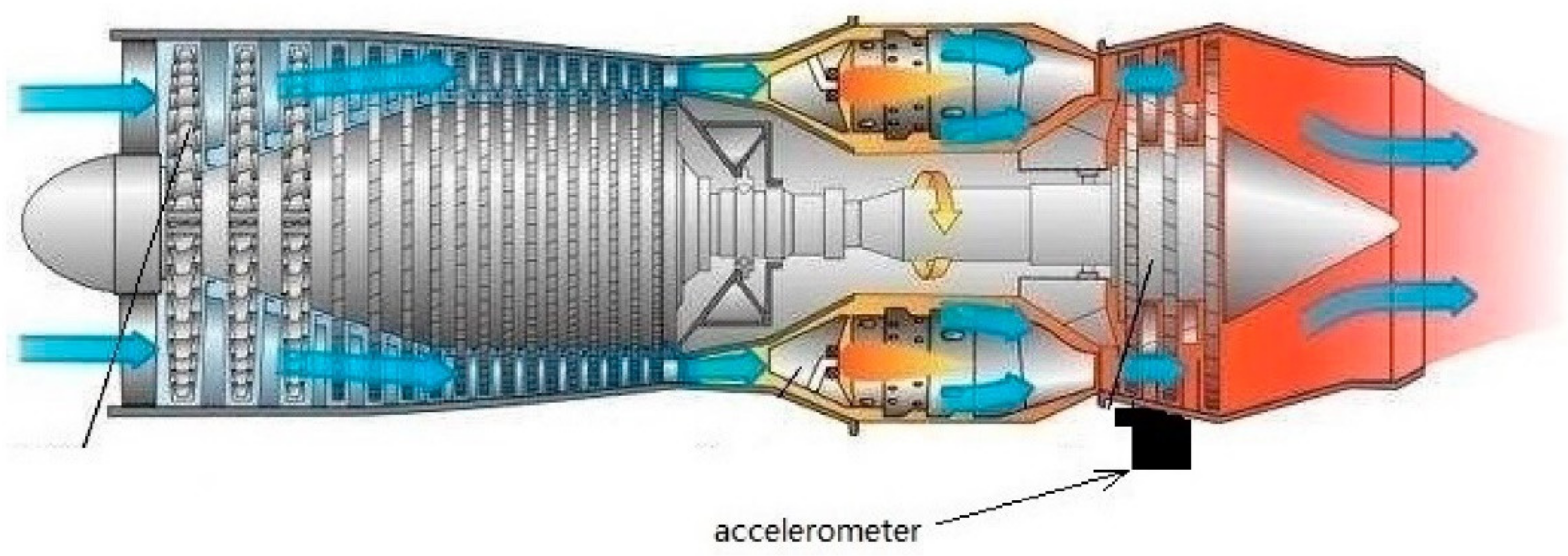
The mounting position of the accelerometer is shown in
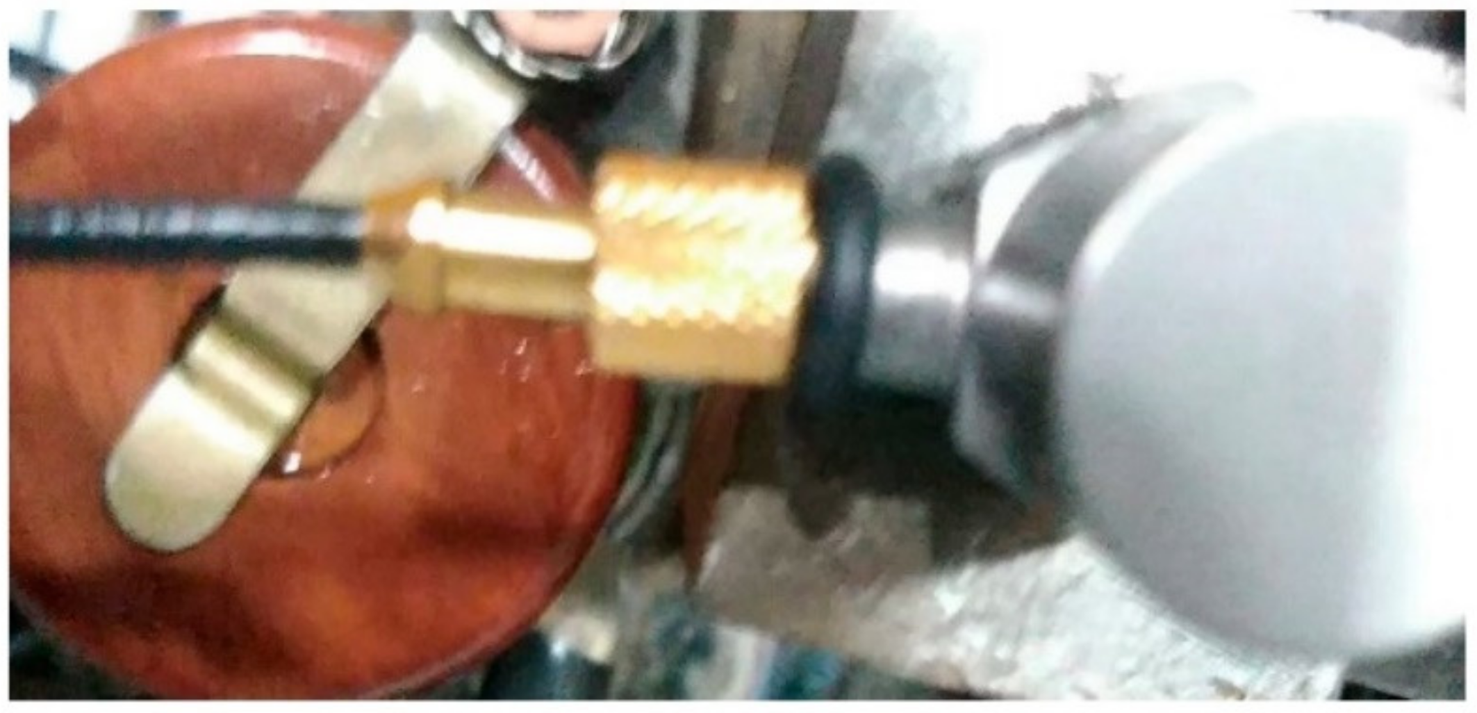
Figure 15. During installation, according to the requirements on the “installation and operating manual of the accelerometer”, the mounting torque is controlled within the range of 113 N.cm to 225 N.cm. A photo of the accelerometer is shown in
Figure 16. The accelerometer was produced by PCB company. Its sensitivity is 1.02 pC/(m/s
2), its frequency range is 9 kHz, its non-linearity ≤1%, its operating temperature range is (−71) °C to 260 °C, and its weight is 11 g. The accelerometer transfers the charge through the cable to the charge converter.
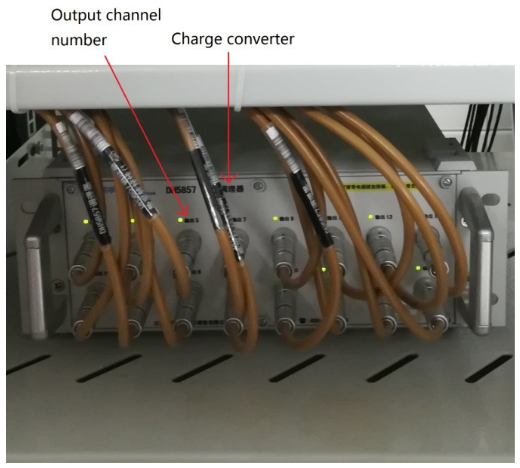
A photo of the charge converter is shown in
Figure 17. The charge converter was produced by DONGHUA company. It has 16 channels, its maximum measurement range is 100,000 pC, its maximum signal output voltage is ±10 V, its current excitation is 2 mA, and its frequency range is 100 kHz. It transfers the voltage through the cable to a data acquisition device.
A photo of the data acquisition device is shown in
Figure 18. The data acquisition device was produced by DONGHUA company. Maximum sampling frequency of the data acquisition device is 1 MHz per channel. It has 16 data acquisition channels and its accuracy is ±0.5%. It has multiple measurement ranges that can be switched; the minimum measurement range is ±5 mV, and the maximum measurement range is ±10 V. It transmits the signal to the computer through the network cable.
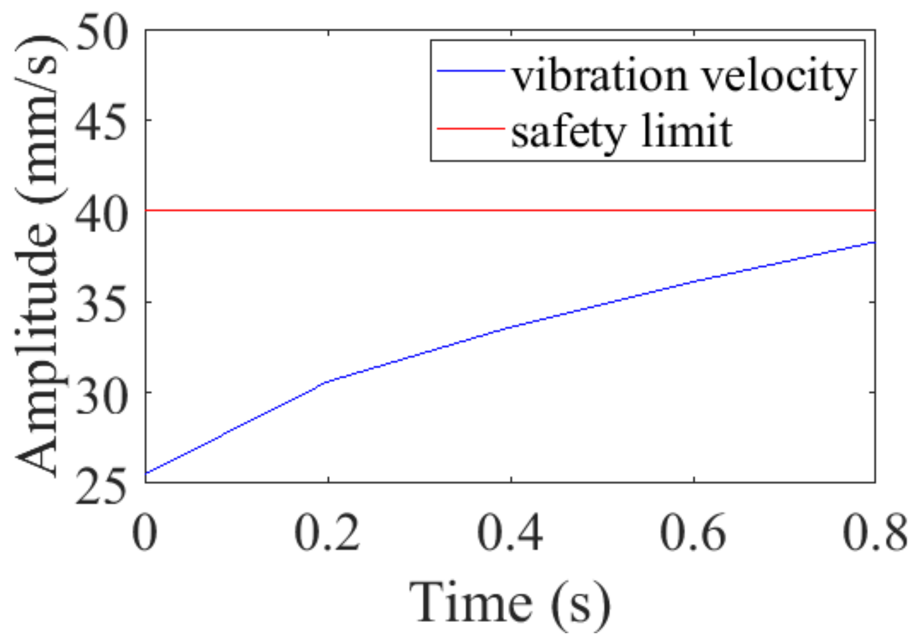
During the aeroengine test, the root mean square (RMS) of vibration velocity almost reached the safety limit, as illustrated in
Figure 19.
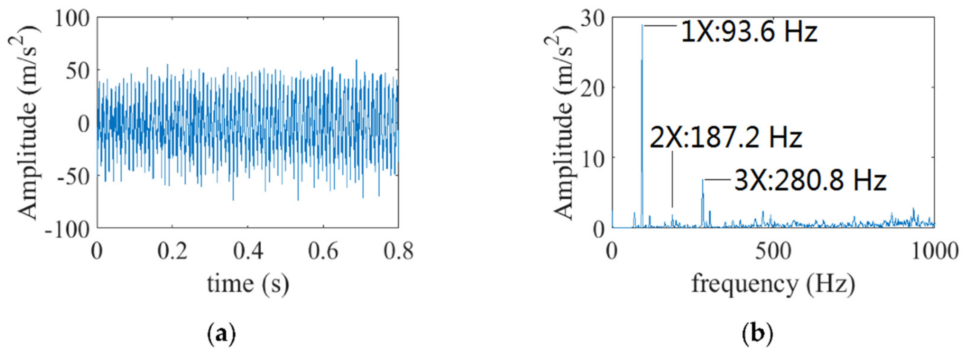
The waveform and Fourier spectrum of the vibration signal obtained from the aeroengine test is revealed in
Figure 20. It is illustrated that there are two frequency peaks with high amplitude, i.e., the rotation frequency of the low-pressure turbine (X), and its three multiples (3×). After comparing with the FFT of the simulated vibration signal in
Figure 8b, it was found that the amplitude of 3× of the vibration signal obtained from simulation is high is very low. During the engine test, the rub-impact occurred more complicated than in the dynamic simulation, and the parameters
,
, etc. in the dynamic simulation were not completely consistent with the parameters in the real aeroengine test.
The raw signal is decomposed into 4 modes using VMD [
18]. u
1(t) is 1×, u
4(t) is 3×. Additionally, u
1(t), u
4(t) are shown in
Figure 21.
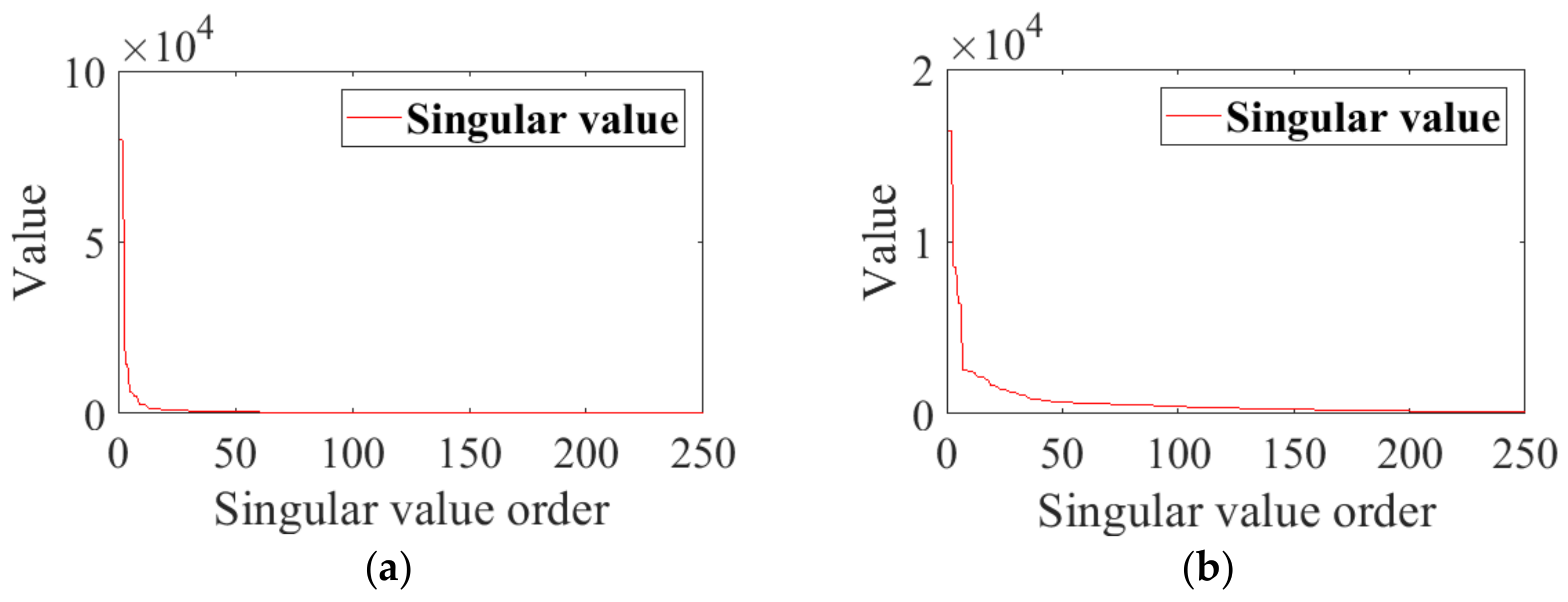
Then, first-layer SVD was applied to u
1(t), u
4(t) for signal denoising. Firstly, the Hankel matrices were constructed. Then, SVD was performed on these two matrices; the first 250 singular values obtained are shown in
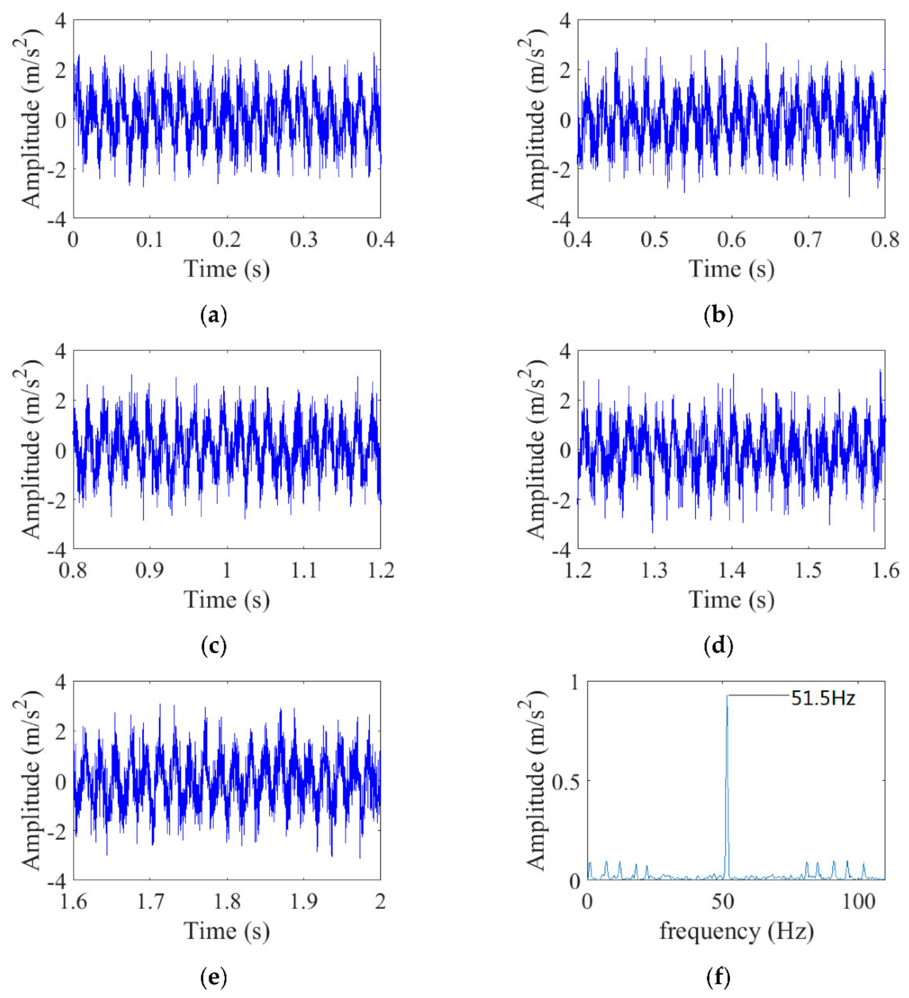
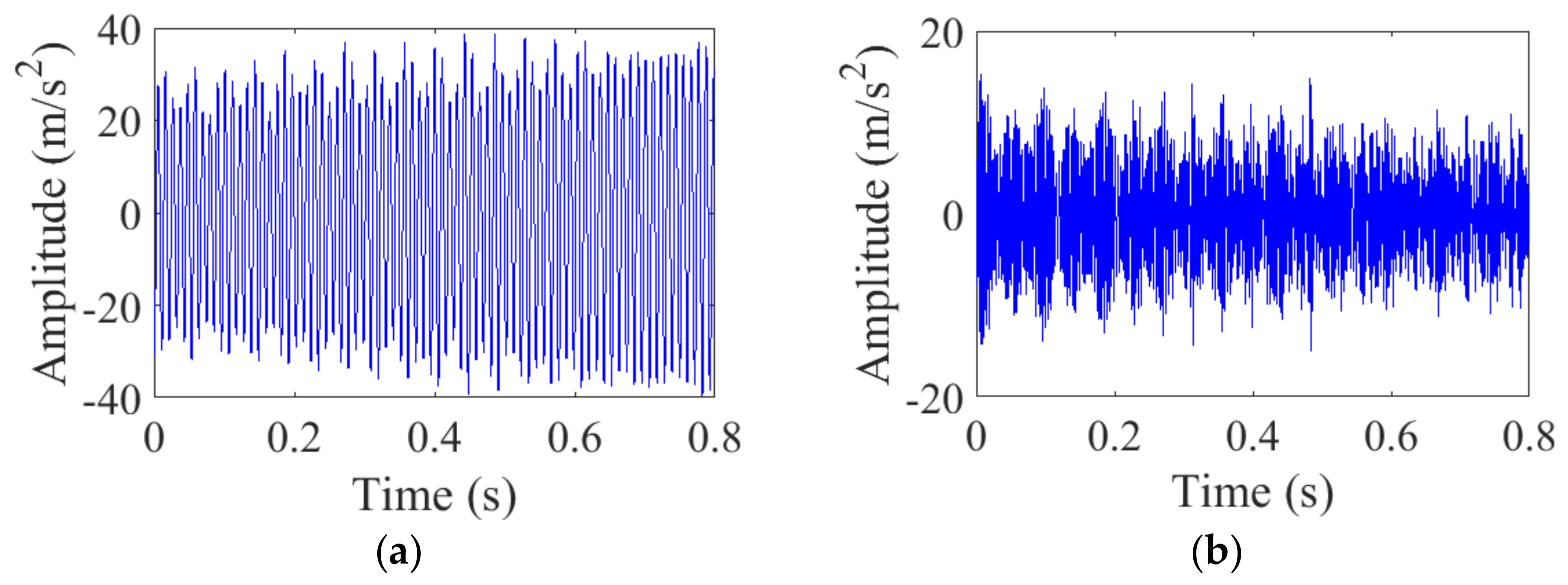
Figure 22. The first 250 largest singular values for matrix reconstruction were then selected, several component matrices were obtained, and the component matrices were superimposed to obtain the reconstruction matrix. Then, the signal from the reconstruction matrix was recovered to obtain the purified signal. C
1(t), C
2(t) are the purified signals of u
1(t), u
4(t), and C
1(t), C
2(t)are shown in
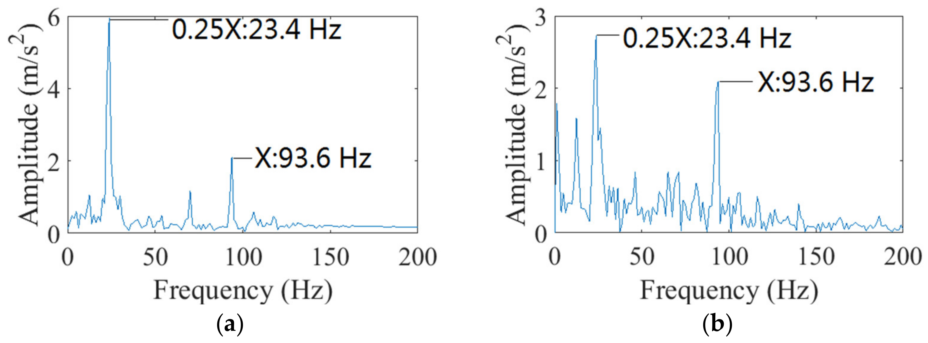
Figure 23. The envelope spectrums for C
1(t) (i.e., 1×) and C
2(t) (i.e., 3×) are revealed in
Figure 24. The main fluctuating frequencies of the envelope of 1× are 23.4 Hz and 93.6 Hz. Additionally, 23.4 Hz is 1/4-times the rotation frequency, 93.6 Hz is the rotation frequency. As for the 3×, the fluctuating frequencies of the envelope of 3× are also 23.4 Hz and 93.6 Hz. After comparing with the simulated vibration signal in
Figure 10b, it is found that the fluctuating frequencies of the envelope of 1×, which was obtained by processing the simulated signal, do not contain 1/4-times the rotation frequency. The fluctuating frequencies of the envelope of 1×, which was obtained by processing the signal of the real aeroengine test, do not contain two-times and three-times the rotation frequency. During the engine test, the rub-impact occurred more complicated than in the dynamic simulation, and the parameters
,
, etc. in the model were not completely consistent with the parameters in the real aeroengine test.
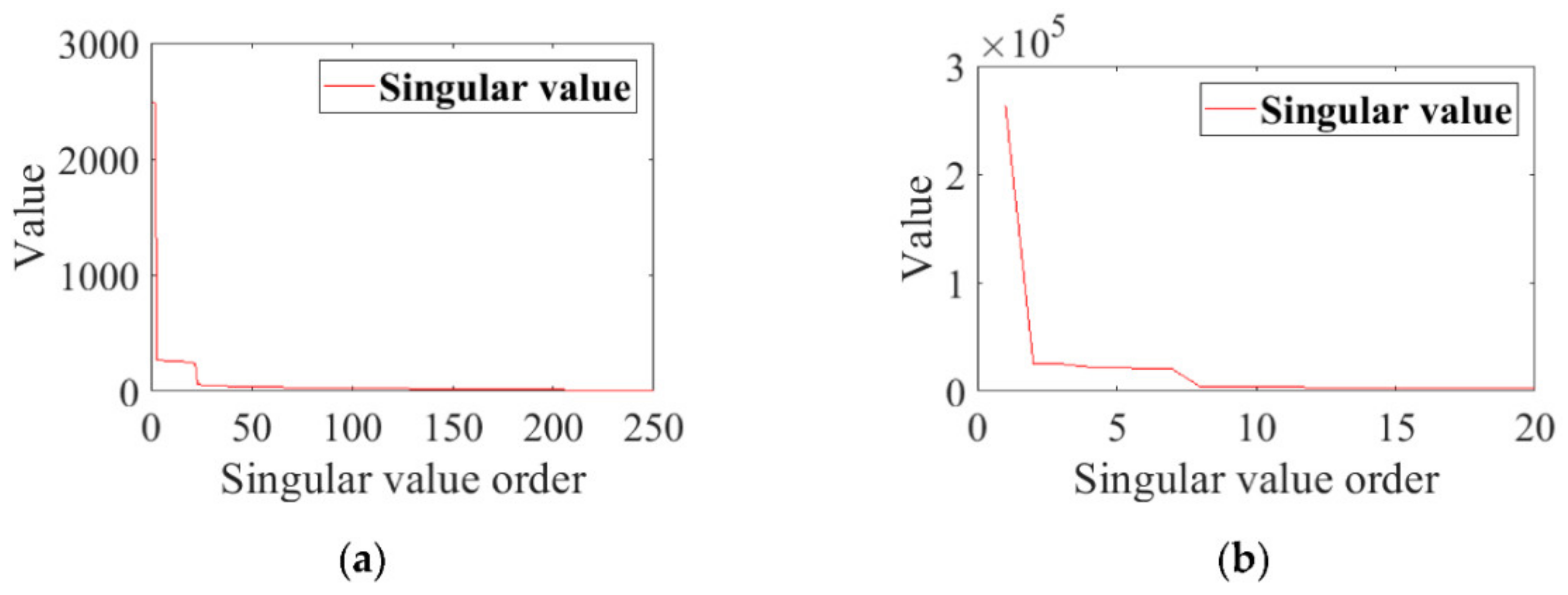
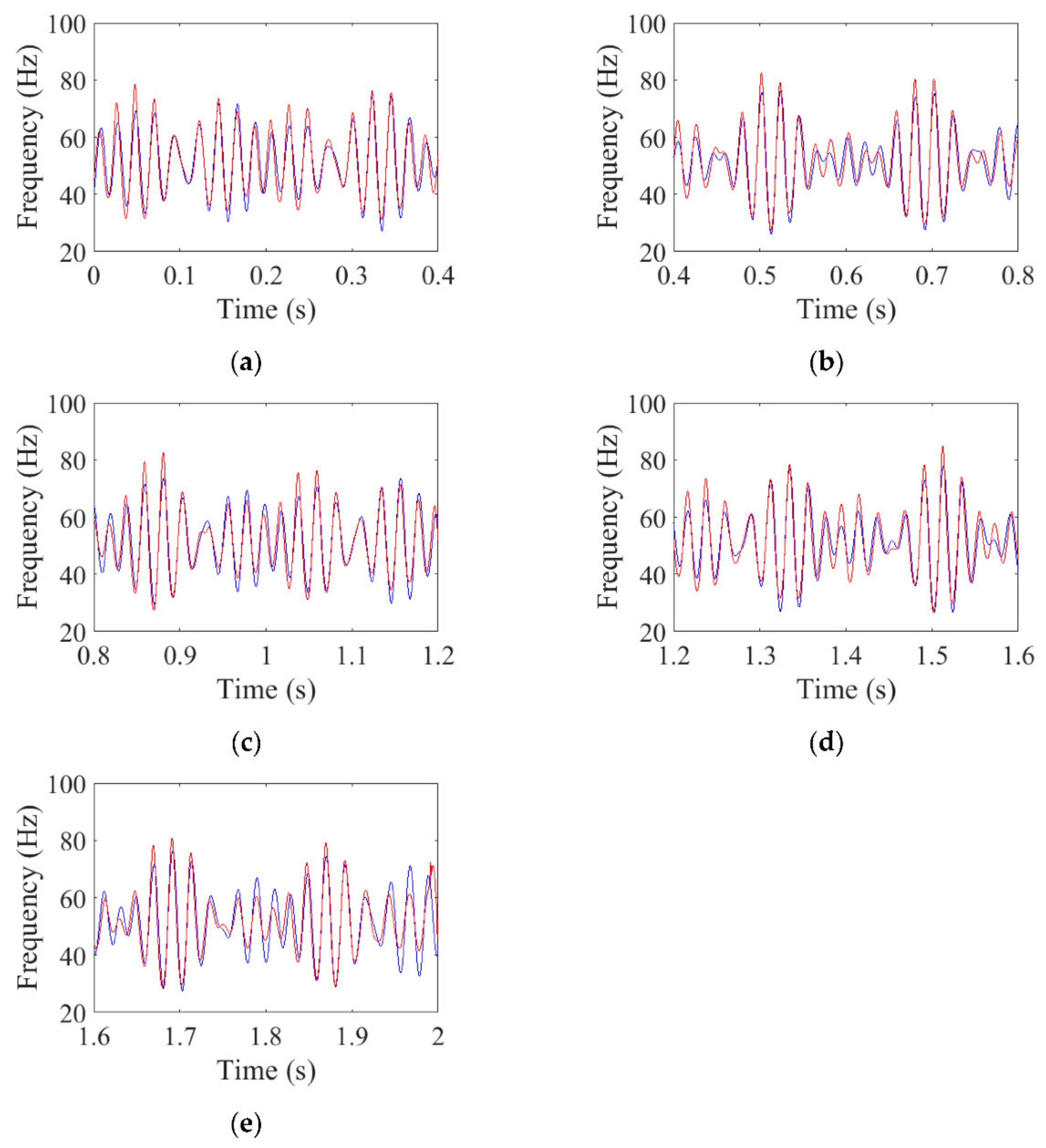
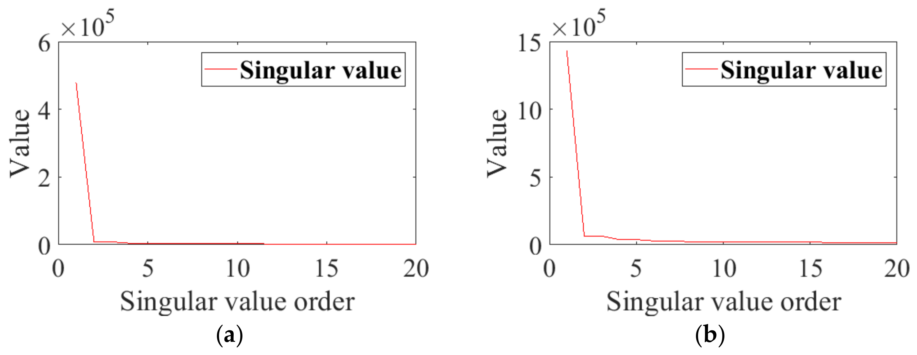
Second-layer SVD was applied to IFs of C
1(t), C
2(t), and the first 20 singular values obtained are shown in
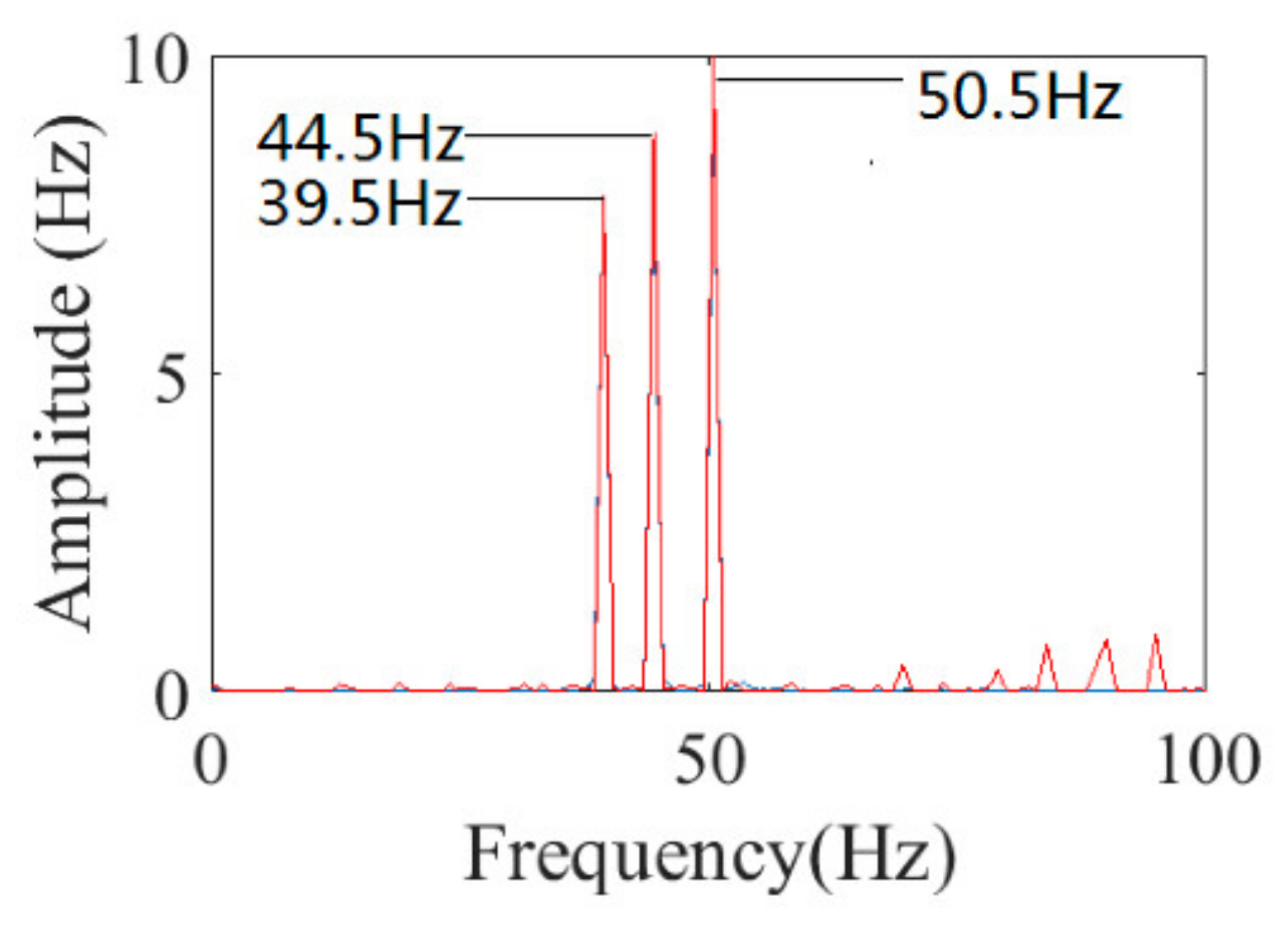
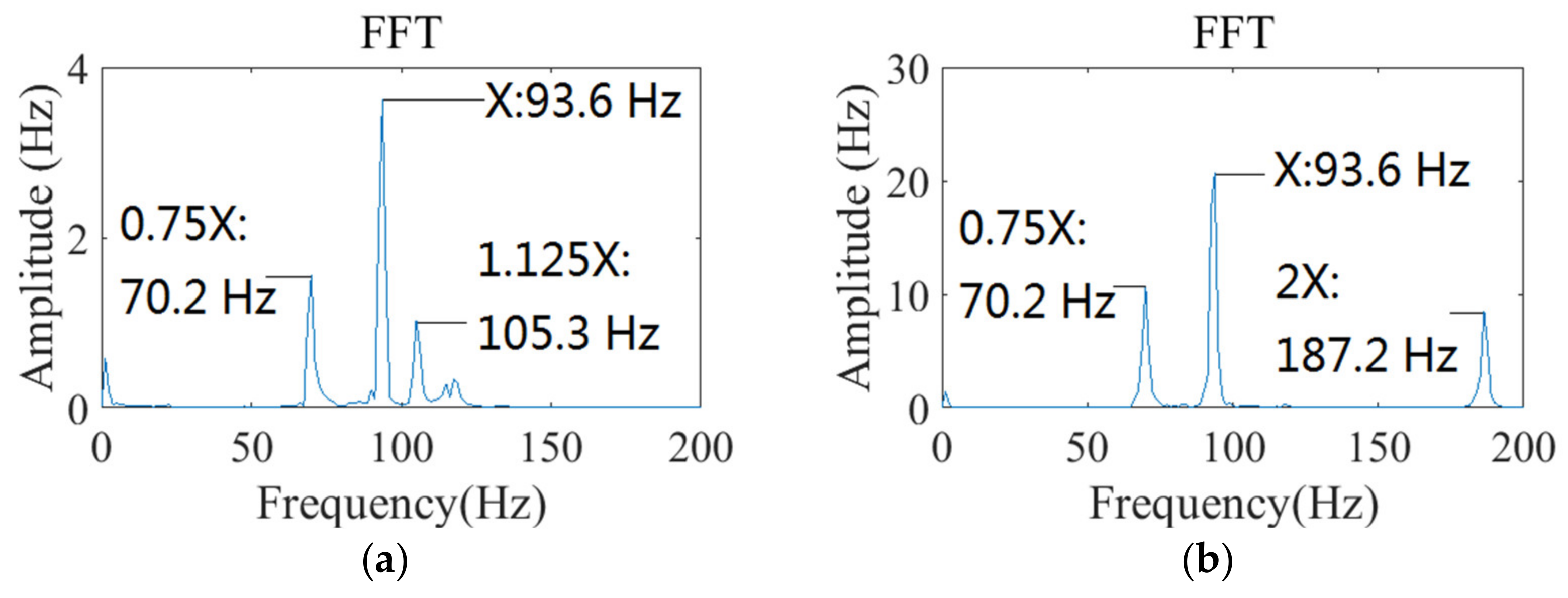
Figure 25. The first seven largest singular values for matrix reconstruction were selected, several component matrices were obtained, and the component matrices were superimposed to obtain the reconstruction matrix. Then, the signal was recovered from the reconstruction matrix. FFT was applied to the IFs of fundamental harmonic (1×) and its three multiples (3×); the FFT of the IFs are revealed in
Figure 26. We can see that the main fluctuating frequencies of the IF of 1× are 70.2 Hz, 93.6 Hz, 105.3 Hz. Additionally, 70.2 Hz is 3/4-times the rotation frequency, 93.6 Hz is the rotation frequency, 105.3 Hz is 9/8-times the rotation frequency. IF, which fluctuates around the rotation frequency, is a feature of rub-impact fault. Additionally, the main fluctuating frequencies of the IF of 3× are 70.2 Hz, 93.6 Hz, 187.2 Hz. Additionally, 70.2 Hz is 3/4-times the rotation frequency, 93.6 Hz is the rotation frequency, 187.2 Hz is two-times the rotation frequency. After comparing with the simulated vibration signal in
Figure 10a, it is found that the fluctuating frequencies of IF of 1×, which was obtained by processing the simulated signal in dynamic simulation, do not contain 3/4-times, and 9/8-times the rotation frequency. The fluctuating frequencies of IF of 1×, which were obtained by processing signal of the real aeroengine test, do not contain two-times the rotation frequency, three-times the rotation frequency, four-times the rotation frequency, and five-times the rotation frequency. During the engine test, the rub-impact occurred more complicated than in the dynamic simulation, and the parameters
,
, etc. in the model were not completely consistent with the parameters in the real aeroengine test.
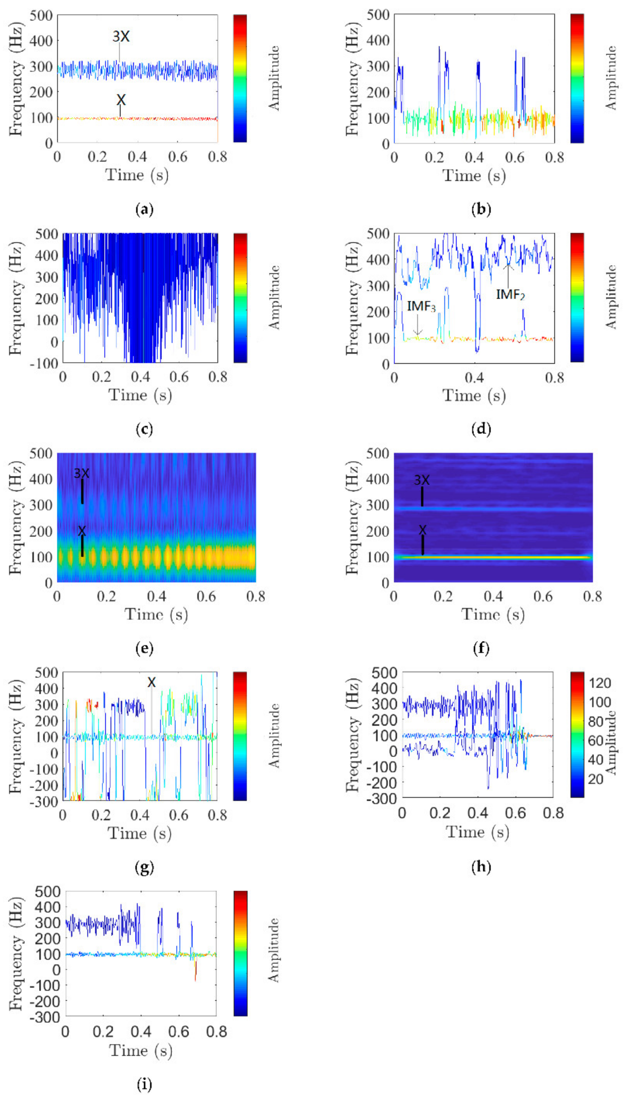
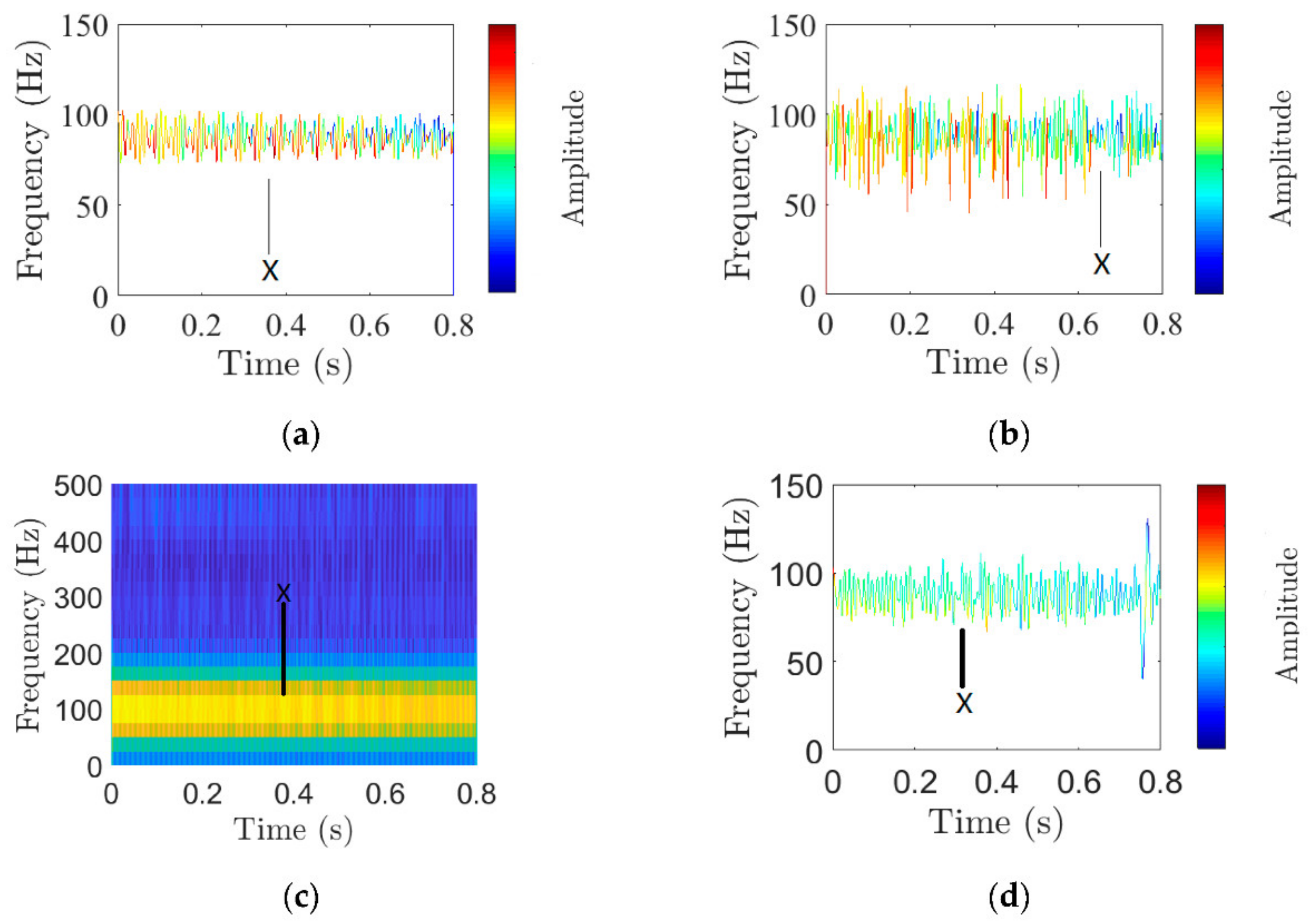
For comparison, the proposed method was used: HHT, STFT, and Nonlinear Chirp Mode Decomposition (VNCMD) on the signal, as shown in
Figure 27. For the VMD method,
was set in advance to determine the number of modes in the data, and
was set to 4. After VMD and two-layer SVD, the Hilbert spectrum of 1× and 3× are shown in
Figure 27a. Compared to
Figure 27b–i, the fluctuating pattern of the IFs are clearly shown in
Figure 27a, and the 1× and 3× can be recognized. The HHT was utilized to analyze the raw signal, which is not purified. The raw signal was decomposed into five IMFs. Only IMF
2, IMF
3, which are related to 1× and 3×, are shown in the Hilbert spectrum. Additionally, the Hilbert spectrum of IMF
3 is shown in
Figure 27b, IMF
3 is almost 1×, IF of IMF
3 fluctuates around 93.6 Hz most of the time. However, it suffers from mode mixing at 0.03 s, 0.21 s, 0.25 s, 0.42 s, 0.60 s and 0.64 s. Additionally, at these times the instantaneous frequency is incorrect. The Hilbert spectrum of IMF
2 is shown in
Figure 27c; the instantaneous frequency of IMF
2 fluctuates irregularly, with a large fluctuation range from 0 s to 0.8 s. The minimum value of its fluctuation is even less than 0 Hz from 0.3 s to 0.5 s, which is obviously wrong. Then, the median filtering was utilized to the IFs and instantaneous amplitudes (IAs); the result is shown in
Figure 27d. IMF
3 is almost 1×, but it suffers from mode mixing. 3× cannot be seen from IMF
2, and the FM feature of IMF
2, IMF
3 disappear. So, signal denoising before Hilbert transform is necessary. The short-time Fourier transform (STFT) was used for the original signal, when the length of the window is 256. Additionally, the result of STFT is shown in
Figure 27e. By comparing
Figure 27a–c,e, it is found that both
Figure 27a,e can successfully show 1× and 3×, whereas
Figure 27b,c do not display 1× and 3× correctly due to noise. However,
Figure 27e has a lower frequency resolution than
Figure 27a. To make the frequency resolution of STFT higher, the length of the window was adjusted to 2560. By comparing
Figure 27a,f, it is found that
Figure 27f cannot show the characteristic of rapid change of instantaneous frequencies. The time–frequency diagram obtained by using STFT cannot guarantee good frequency resolution and the fast-changing instantaneous frequency can be displayed at the same time, no matter how we adjust the length of the window. In fact, the time–frequency diagram obtained by this method cannot guarantee good time resolution and frequency resolution [
29]. Applying VNCMD to the signal, when using this method, the number of signal components needs to be set to K in advance [
30,
31,
32], when K is set equal to 2, the decomposition result is shown in
Figure 27g. 1× is correctly decomposed, but 3× cannot be seen. When K is set to 3, the VNCMD result is shown in
Figure 27h. It can be seen that the instantaneous frequency of 1× is wrong at 0.65 s, and 0.72 s, and the instantaneous frequency of 3× is wrong from 0.62 s to 0.8 s. When K is set to 4, the VNCMD result is shown in
Figure 27i. The first three modes almost overlap each other, and their center frequency is all 93.6 Hz, and the instantaneous frequency of 3× is wrong from 0.4 s to 0.8 s.
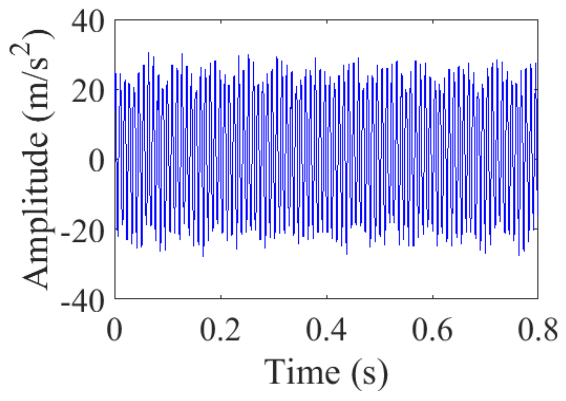
Next, we analyzed the second set of fault data, when the speed of the low-pressure turbine is about 6660 r/min (111.0 Hz). The waveform of the vibration signal is shown in
Figure 28a, The FFT of the vibration signal is shown in
Figure 28b. After comparing with the simulated vibration signal in
Figure 11b, it is found that the Fourier spectra of the dynamic simulation signal and the aeroengine test signal are relatively similar, with higher 1× amplitudes and lower 2× and 3× amplitudes.
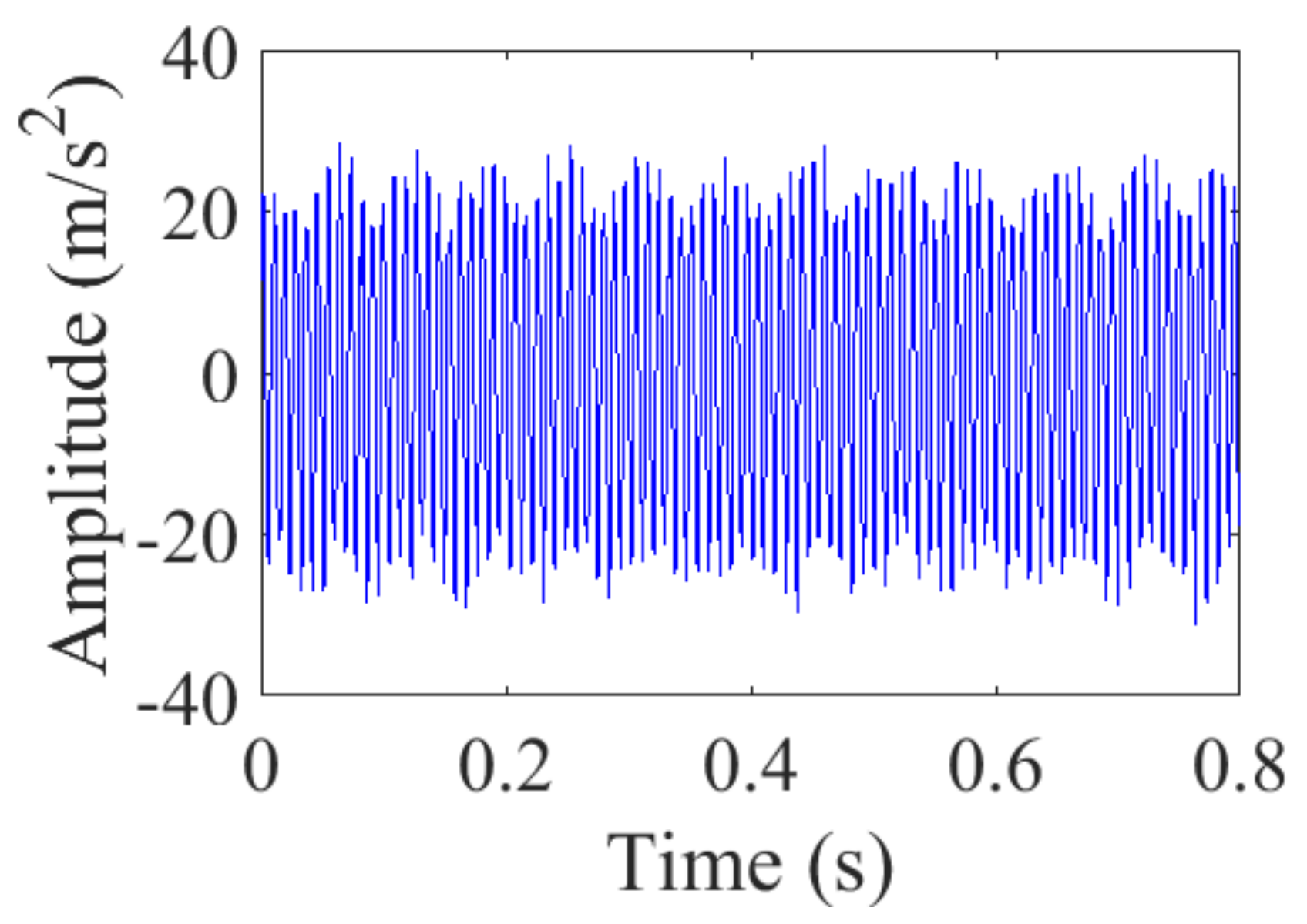
The raw signal is decomposed into two modes using VMD. D
1(t) is 1×. Additionally, D
1(t) is shown in
Figure 29.
The first layer SVD was performed to denoise D
1(t) and retain the first 250 singular value components; the first 250 singular values obtained are shown in
Figure 30. The signal after denoising is E
1(t), E
1(t) is shown in
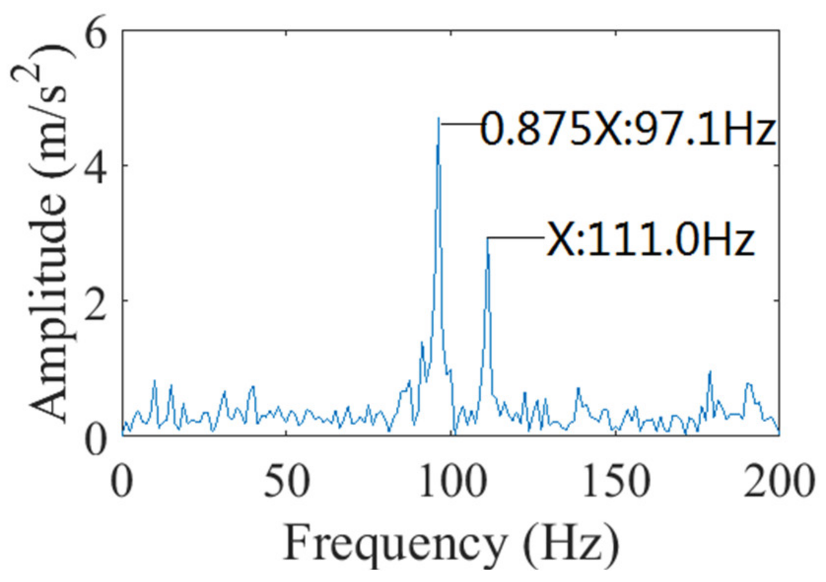
Figure 31 The envelope spectrum of the signal after signal denoising is shown in
Figure 32. It can be seen that the main fluctuating frequencies of 1× on the envelope spectrum are 97.1 Hz and 111.0 Hz. Additionally, 97.1 Hz is 7/8-times the rotation frequency and 111.0 Hz is equal to the rotation frequency. After comparing with the simulated vibration signal in
Figure 13b, it is found that the fluctuating frequencies of the envelope of 1×, which is obtained by processing the simulated signal, do not contain 7/8-times the rotation frequency. The fluctuating frequencies of the envelope of 1×, which were obtained by the processing signal of the real aeroengine test, do not contain two-times the rotation frequency. During the engine test, the rub-impact occurred more complicated than in the dynamic simulation, and the parameters
,
, etc. in the model were not completely consistent with the parameters in the real aeroengine test.
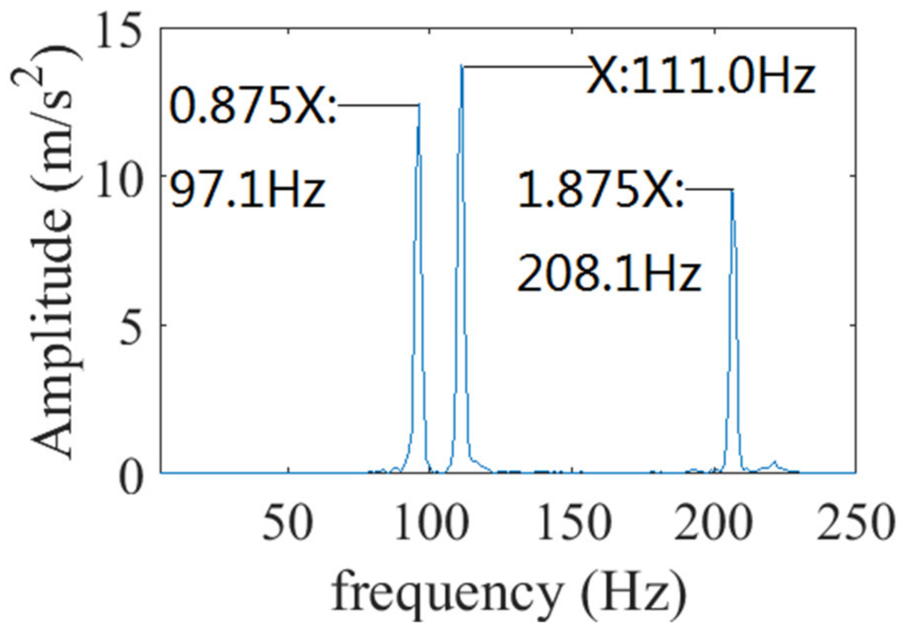
The second layer SVD was performed on the instantaneous frequency. The FFT of the instantaneous frequency is shown in
Figure 33. It can be seen that the fluctuating frequencies of the instantaneous frequency are mainly 97.1 Hz, 111.0 Hz, and 208.1 Hz, which are, respectively, equal to 7/8-times, one-time, and 15/8-times the rotation frequency. Moreover, the fluctuating frequencies of the instantaneous frequency of 97.1 Hz and 111.0 Hz are consistent with the fluctuating frequencies on the envelope spectrum. IF fluctuating around the rotation frequency is a feature of rub-impact fault, and it can identify rub-impact fault more clearly than the lower amplitude 2×, 3× in Fourier spectrum in
Figure 28b. After comparing with the simulated vibration signal in
Figure 13a, it is found that the fluctuating frequencies of IF of 1×, which was obtained by processing the simulated signal in dynamic simulation, do not contain 7/8-times, and 15/8-times the rotation frequency. The fluctuating frequencies of IF of 1×, which was obtained by the processing signal of the real aeroengine test, do not contain two-times the rotation frequency, and three-times the rotation frequency. During the engine test, the rub-impact occurred more complicated than in the dynamic simulation, and the parameters
,
, etc. in the model were not completely consistent with the parameters in the real aeroengine test.
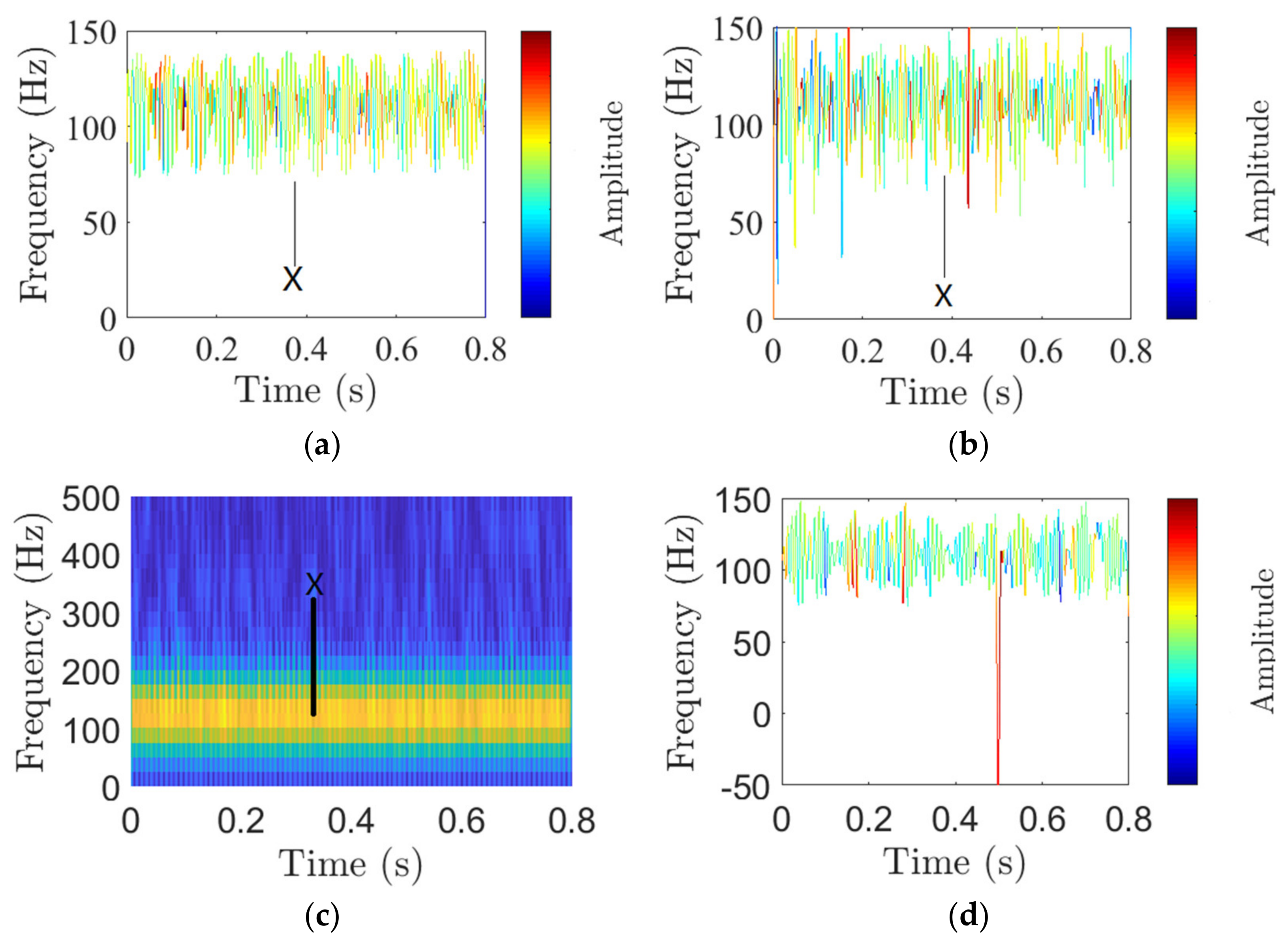
For comparison, the proposed method was used; HHT, STFT, VNCMD, on the signal, as shown in
Figure 34. Using the proposed method, the instantaneous frequency result obtained is very good, as shown in
Figure 34a. It can be clearly seen that the instantaneous frequency is the sum of several sinusoids. After using HHT, 1× is decomposed, as shown in
Figure 34b. However, the instantaneous frequency fluctuates irregularly, with a large fluctuation range around 0 s, and a small fluctuation range around 0.8 s. The STFT result of the signal is shown in
Figure 34c. 1× is shown in the time–frequency diagram. The time–frequency diagram obtained by this method cannot guarantee good time resolution and frequency resolution [
29]. Directly using VNCMD on the signal, the number of signal components was set to K equal to 2, and 1× was almost decomposed, as shown in
Figure 34d, but the result at 0.5 s on the time–frequency diagram is wrong.
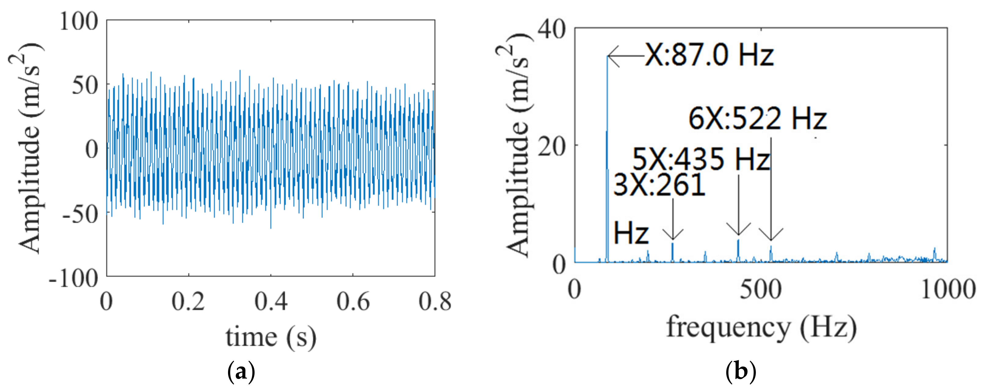
Next, let us analyze the third set of data. At this time, the speed of the low-pressure turbine is 5220 r/min (87.0 Hz), and the waveform of the vibration signal is shown in
Figure 35a. The FFT of the vibration signal is shown in
Figure 35b, the amplitude of 1× is high, amplitudes of 2× to 6× are low.
The raw signal is decomposed into two modes using VMD. F
1(t) is 1×, the waveform of the F
1(t) is shown in
Figure 36.
The first layer of SVD was performed on F
1(t) for signal denoising, and the first 250 singular value components retained, and the first 250 singular values obtained are shown in
Figure 37. The signal after denoising was G
1(t), and G
1(t) is shown in
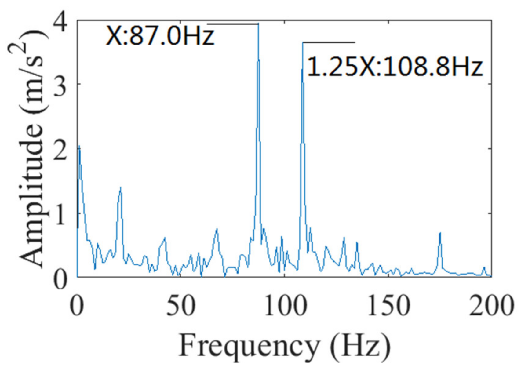
Figure 38. The envelope spectrum of the signal after denoising is shown in
Figure 39. It can be seen that the main fluctuating frequencies of 1× on the envelope spectrum are 87.0 Hz and 108.8 Hz. Additionally, 87.0 Hz is equal to the rotation frequency, 108.8 Hz is 5/4-times the rotation frequency.
The second layer SVD is performed on the instantaneous frequency. The FFT of the instantaneous frequency is shown in
Figure 40. It can be seen that the fluctuating frequencies of the instantaneous frequency are mainly 87.0 Hz, 108.8 Hz, and 174 Hz, which are, respectively, one-time, 5/4-times, and two-times the rotation frequency. IF fluctuating around the rotation frequency is a feature of the rub-impact fault. Moreover, the fluctuating frequencies of the instantaneous frequency are 87.0 Hz and 108.8 Hz, which are consistent with the fluctuating frequencies on the envelope spectrum.
For comparison, the proposed method was used; HHT, STFT, VNCMD, on the signal, as shown in
Figure 41. Using the proposed method, the instantaneous frequency result obtained was very good, as shown in
Figure 41a. It can be clearly seen that the instantaneous frequency is the sum of several sinusoids. After using HHT, 1× was decomposed, as shown in
Figure 41b. However, the instantaneous frequency fluctuates irregularly. The STFT result of the signal is shown in
Figure 41c. You can see 1× in the time–frequency diagram. The time–frequency diagram obtained by this method cannot guarantee good time resolution and frequency resolution [
29]. Using VNCMD on the signal, the number of signal components was set K equal to 2, and 1× was also decomposed, as shown in
Figure 41d.


 ,
, 


