Application of Remote Sensing Tools to Assess the Land Use and Land Cover Change in Coatzacoalcos, Veracruz, Mexico

Abstract

Land use and land cover (LULC) change has become an important research topic for global environmental change and sustainable development. As an important part of worldwide land conservation, sustainable development and management of water resources, developing countries must ensure the use of innovative technology and tools that support their various decision making systems. This study provides the most recent LULC change analysis for the last six years (2015–2021) of Coatzacoalcos, Veracruz, Mexico, one of the most important petrochemical cities in the world and host of the ongoing Interoceanic Corridor project. The analysis was carried out using Landsat 8 Operational Land Imager (OLI) satellite images, ancillary data and ground-based surveys and the Normalized Difference Vegetation Index (NDVI) to identify and to ameliorate the discrimination between four main macro-classes and fourteen classes. The LULC classification was performed using the maximum likelihood classifier (MLC) to produce maps for each year, as it was found to be the best approach when compared to minimum distance (MDM) and spectral angle mapping (SAM) methods. The macro-classes were water, built-up, vegetation and bare soil, whereas the classes were an improved classification within those. Our study achieved both user accuracy (UA) and producer accuracy (PA) above 90% for the proposed macro-classes and classes. The average Kappa coefficient for macro-classes was 0.93, while for classes it was 0.96, both comparable to previous studies. The results from the LULC analysis show that residential, industry and commercial areas slowed down their growth throughout the study period. These changes were associated with socio-economical drivers such as insecurity and lack of economic investments. Groves and trees presented steady behaviors, with small increments during the five-year period. Swamps, on the other hand, significantly degraded, being about 2% of the study area in 2015 and 0.93% in 2021. Dunes and medium and high vegetation densities ($\sim 80\%$) transitioned mostly to low vegetation densities. This behavior is associated with rainfall below the annual reference and increments of surface runoff due to the loss of vegetation cover. Lastly, the present study seeks to highlight the importance of remote sensing for a better understanding of the dynamics between human–nature interactions and to provide information to assist planners and decision-makers for more sustainable land development.

1. Introduction

Land use and land cover (LULC) changes are among the research topics more recurrent in remote sensing [1,2,3,4]. Remote sensing provides comprehensive and extensive information to understand the interaction between terrestrial ecosystems and their responses to environmental factors [5,6,7,8,9,10,11]. This technology is considered a powerful source to obtain information from terrestrial surface characteristics at different temporal and spatial scales [12,13,14,15,16]. For more than half a century, scientists have used several types of remote sensing data. From those, the most commonly used source is the Landsat satellite based-data [17]. One of main uses of the Landsat-based satellite images is the identification or classification of LULC changes [18,19,20,21,22]. Some interesting conclusions have been driven through the use of remote sensing in LULC changes. It has been observed that changes in land uses are dynamic, non-linear interactions between humans and nature and are driven by complex stochastic processes [23]; worldwide changes in LULC for the last 300 years have shown gains in agriculture and losses in forest [24]; rapid population growth in Africa has been identified as the main driving force for the expansion of agricultural land, whereas in developing countries, urbanization dynamics are attributed to demographic factors [25] and transitions from cropland to urban and water bodies areas have been identified as an important trend in Europe [26].

Some of the more remarkable research found in literature is the work conducted by Yuan et al. [27]. Their research consists of the use of multi-temporal Landsat Thematic Mapper data to map and quantify the LULC changes in seven counties of the Twin Cities located in the metropolitan area of the state of Minnesota, United States. They used satellite images corresponding to the years 1986, 1991, 1998 and 2002. Yuan et al. demonstrated an urban zone increment from 23.7 to 32.8% in the study area. Surfaces such as rural areas, croplands, forests and wetlands decreased from 69.6 to 60.5%. Another unique example is the work carried out by Demissie et al. [28], where Landsat satellite data from 1973 to 2015 were classified to study land use change and its possible causes in Gonder, Ethiopia. The study showed that about 60.1% of the area experienced land use changes within the study period.

In Mexico, little research related to the quantification of LULC changes has been found within the literary review. One of the few works found was carried out by Colditz et al. [29]. Their research presents a methodology to develop a land use map in Mexico for the year 2005. The scheme was based on time series from a Moderate Resolution Imaging Spectroradiometer (MODIS) with a 250 m resolution and an extensive sampling of data for the different geographic zones of the Mexican surface. The results showed a map with an overall precision of 82.5% (Kappa statistic = 0.79). A further evaluation with 780 randomly generated samples within the classes with referenced field data indicated a precision equal to 83.4% (Kappa statistic = 0.80). Another study found in the literature includes the generation of a land use map of the Latin American and Caribbean zone for the year 2008. This project was developed within the framework of the project of the Latina American Network for Monitoring and Studying of Natural Resources (SERENA) [30]. Similar to Colditz et al. [29], time series and decision trees with MODIS data (250 m) were used for the classification of land use changes. The discrete SERENA model showed an overall accuracy of 84%. Other uses of remote sensing in Mexico include the detection of chinampas in the Xaltocan area in the Northern Basin of Mexico [31], the evolution of sea temperature on the west coast of Baja California [32] and/or hydropower assessment [33].

Due to the limitations observed in the use of remote sensing in Mexico, such as limited research using remote sensing and map course resolution, this study has integrated remote sensing, Geographic Information Systems (GIS) analysis, field sampling and image revision to assess the potential of the use of Landsat 8 satellite data to assess and monitor land use changes and coverage changes in the southeastern region of the state of Veracruz, Mexico, located in the southern coastal area of the Gulf of Mexico. Three widely used classification methods are explored to select the more appropriate algorithm for LULC classification under the same level of information previously extracted from field data, digital maps and ancillary data. This comparison allows for conclusions on the advantages and drawbacks of current classification algorithms. The analysis encompasses the definitions of macro-classes of land use and their derived classes. The Normalized Difference Vegetation Index, also known as NDVI, was used to identify and improve discrimination between macro-classes and classes within the study area. A supervised classification method, the Maximum Likelihood Classification (MLC), was applied in this study due to its availability within the GIS applications in addition to it not requiring an extensive training process [34,35]. The most important advantage of the MLC as a parametric classifier is that it takes into account the variance within the selected classes and that, for normally distributed data, the MLC method performs a better qualification than other methods, namely, decision trees [34,36].

Additionally, this study proposes a methodology to obtain updated temporal information of the change in land use and land cover for the Coatzacoalcos area using Landsat 8 satellite imagery, which has a higher resolution with the available MODIS maps. The mapping of land use and its changes are critical and important factors for sustainable development as well as the monitoring of environmental impacts. The final product of this research will help government agencies to make decisions on urban development and preservation of available natural resources, since one of the emblematic projects in Mexico known as the Interoceanic Corridor is being executed in the present year. Lastly, this piece of research is going to serve as the baseline for additional contributions on LULC change prediction with more complex analyses of the drivers forcing these landscape modifications.

2. Materials and Methods

2.1. Study Area

The study area is the southeastern region of the state of Veracruz, Mexico, in which one of the most important pretrochemical ports of the country is located at the city of Coatzacoalcos. This city is surrounded by the Coatzacoalcos and Tonalá rivers and extends between latitudes 18.06${}^{\circ }$ and 18.21${}^{\circ }$ and longitudes −94.22${}^{\circ }$ and −94.64${}^{\circ }$ (Figure 1). The area of study extends over an area about 220 km${}^2$. The port of Coatzacoalcos is dominated by the petrochemical sector [37]. Four of the petrochemical complexes located near the city make the city one of the most important oil areas in the world [38]. Coatzacoalcos has been a transportation hub for hundreds of years; it is connected by air, land, sea and railroad to the rest of the world. Currently, the Mexican government is working on a project called the Interoceanic Corridor of the Isthmus of Tehuantepec, which represents the modernization and installation of industrial parks inside the industrial areas of the ports of Coatzacoalcos and Salina Cruz, Mexico [39]. This project will represent economic and population growth within the city. As a result, land use assessments and projections have become priorities to help both state and federal government make decisions for the projected economical growth.

Physiographically, the study area has an average elevation of 10 meters above sea level. The soils found in the region are clayey lateritic Acrisol and Luvisol in high elevations and Gleysol, Cambisol, Vertisol and Nitosol in plains [40]. The vegetation consists of riparian vegetation, swamps and wetlands in floodable areas, mesophilic mountain pine oak forests in high areas and high evergreen forests in hills and acahual areas in abandoned and cultivated pastures. The climate of the region is a warm humid climate with abundant rains in summer. The average annual temperature varies between 24 and 25 °C, while the average annual precipitation varies between 1500 and 2500 mm [41].

2.2. Data Acquisition and Processing

The images used in this study were obtained from the Landsat 8 satellite, which captures multispectral images of 30 m resolution sampled with the OLI (Operational Land Imager) sensor. The Landsat 8 satellite also provides a 15 m panchromatic band, allowing for a greater spatial resolution. All images were geometrically corrected and acquired in level 1 (L1). The images can be directly downloaded from the EarthExplorer gateway of the United States Geological Survey (USGS) [17].

Table 1. Images of Landsat 8 OLI used in the present study.

Satellite	Acquisition Date	Bands	Spectral Resolution	Path/Row	Cloudiness
Landsat 8 OLI	14/06/2015	2–7	30 m	023/047	30%
Landsat 8 OLI	26/06/2016	2–7	30 m	023/047	25%
Landsat 8 OLI	02/06/2017	2–7	30 m	023/047	9%
Landsat 8 OLI	23/06/2018	2–7	30 m	023/047	13%
Landsat 8 OLI	10/06/2019	2–7	30 m	023/047	0%
Landsat 8 OLI	12/06/2020	2–7	30 m	023/047	5%
Landsat 8 OLI	23/06/2021	2–7	30 m	023/047	0%

displays the details of the images used in this study.

The Landsat 8 OLI products used consist of band 2 (0.45–0.51 µm), band 3 (0.53–0.59 µm), band 4 (0.64–0.67 µm), band 5 (0.85–0.88 µm), band 6 (1.57–1.65 µm) and band 7 (2.11–2.29 µm) [42]. All images were processed using the free software Quantum GIS (QGIS) version 3.14.16. Atmospheric correction was performed through the Semi-Automatic Classification Plugin (SCP) tool based on the Dark Object Subtraction (DOS1) algorithm [43]. The panchromatic band was used to provide higher spatial resolution. This is achieved using Gram–Schmidt Pan-Sharpening to produce a high-resolution color image that improves the training set and the classification process. Google Earth images were acquired according to acquisition dates (Table 1) and geoferenced using QGIS. The closest dates to the acquisition date were selected. Field data included collection of georeferenced points and their corresponding land use for the last two years of the analyzed periods. Figure 2 shows the methodology used for the study.

The DOS1 atmospheric correction method was selected, as it is the most widely used method for LULC change detection [42]. This method uses the properties of the images. For instance, pixels conforming elements such as shadows, water or forests are considered dark objects when the magnitude of the reflectance is close to zero, namely, when the reflectance is less than or equal to 1%, and all the analyzed pixels are assumed dark elements. This assumption indicates that pixels receiving low values of solar radiation (∼100% shade) registered by the satellite correspond to atmospheric dispersion, which generally is caused by effects of the topography [44]. Once a dark object is found in the image, the minimum reflectance value of the total Digital Number (DN) histogram is assigned to the object. This minimum is then modified by the effects of atmospheric correction [45]. The surface reflectance is calculated using the following expression:

$${\rho }_s=\frac{\pi (L_{\mathsf{\lambda }}-L_p)d^2}{ESU{N}_{\mathsf{\lambda }}cos{\theta }_s}$$

(1)

where ${\rho }_s$ is the surface reflectance, d is the distance to the sun, $ESU{N}_{\mathsf{\lambda }}$ is the mean solar exo-atmospheric irradiance, $L_{\mathsf{\lambda }}$ is the solar spectral radiance to the satellite, ${\theta }_s$ is the zenith angle and ${\mathsf{\lambda }}_p$ is the path radiance given by [46]

$$L_p=L_{min}-L_{DO1\%}$$

(2)

where $L_{min}$ is the radiance corresponding to a digital count value for which the sum of all the pixels with digital counts lower than or equal to this value is equal to 0.01% of all the pixels from the image considered [46] and $L_{DO1\%}$ is the radiance of Dark Object assumed to have reflectance value of 0.01.

2.3. NDVI Classification

Based on the interpretation of the Normalized Difference Vegetation Index (NDVI), the analysis of Google-Earth-extracted images, RGB (red, green, blue) images, panchromatic bands and ground-based georeferenced information, NDVI thresholds were proposed to classify the area of study into four macro-classes during the analysis period (2015–2021), as shown in

Table 2. Suitable NDVI ranges identified for the LULC macro-classes.

Macro-Class	NDVI Range
Water	−0.010–−0.133
Built-up	0.040–0.232
Bare soil	0.145–0.259
Vegetation	0.694–0.895

.

The NDVI thresholds implemented in the proposed classification were selected after an extensive literature review of previous studies where the NDVI was used as the spectral index of diverse land covers [47,48,49,50,51,52]. The NDVI values were calculated by the equation proposed in [53,54]:

$$NDVI=\frac{{\varphi }_{nir}-{\varphi }_{red}}{{\varphi }_{nir}+{\varphi }_{red}}$$

(3)

where ${\varphi }_{nir}$ is the near-infrared reflectance and ${\varphi }_{red}$ is the red-band reflectance. Band 4 (0.64–0.67 µm) and band 5 (0.85–0.88 µm) represent ${\varphi }_{nir}$ and ${\varphi }_{red}$, respectively, in the Landsat products. The NDVI values vary from −1 to 1. Values close to 1 represent vegetation in optimal environmental conditions, whereas low values of NDVI indicate low vegetation density or a different land use. After the macro-class definition, a second classification was performed to refine the LULC characteristics through a more extensive discrimination of pixels. These new classes were defined according to the CORINE land cover inventory proposed by the European Environmental Agency [55]. This classification process required the use of the ancillary data and field data to assign new information to the training set. This assignation was repeated until a suitable spatial distribution was obtained. This new classification consisted of 14 classes, as shown in

Table 3. Land use and land cover (LULC) classes and descriptions.

LULC Type	Description
Water
Sea	Area of salt water that surrounds landmasses
Water courses	Natural or artificial water courses serving as water drainage channels
Water bodies	Natural or artificial water bodies with presence of standing water surface during most of the year
Built-up
Industry	Any factory processing of raw materials and manufacture of goods
Residence	Land use in which housing predominates
Commercial	Areas for retail sales, services, offices, etc.
Roads	Roads of any artificial paved surface material (asphalt or concrete)
Vegetation
Mixed forest	Vegetation formation composed principally of trees, including shrub and bush understorey
Shrub	A shrub or clump of shrubs with stems of moderate length
Wetland	Areas of low-lying, uncultivated ground where water collects
Bare soil
Dune	A mound of sand or other loose sediment formed by the wind
Bare surfaces	Soil with low vegetation density
Sparse vegetation	Soil with a mix of low and high vegetation densities
Grassland	Soil with high vegetation density, such as grasslands

.

2.4. Classifier Comparison

In addition to its social and environmental objectives, this study seeks to evaluate the potential and the drawbacks of the minimum distance classifier [56], the spectral angle mapping classifier [57] and the maximum likelihood classifier [34,35,58] in deriving information on LULC. Although there are more classifications, such as artificial neural networks [34] and parallelepiped classification [56], the comparison was limited to the three selected methods because they are often used to classify LULC. However, limited information exists when the same training input and ancillary data are used to perform the classification process. Here, the comparison was set under the assumption that the same amount of information was available.

2.4.1. Minimum Distance Classifier

The minimum distance method (MDM) calculates the Euclidean distance $d(x,y)$ between the spectral signatures given in the training data set and the spectral signatures of the image pixels. The spectral distance is calculated through the following expression:

$$d(x,y)=\sqrt{\sum _{i=1}^n{(x_i-y_i)}^2}$$

(4)

where x is the spectral signature vector of an image, y is the spectral signature vector of the training area and n is the number of bands of the image. Once the spectral distance is computed for every pixel, the class with the closest spectral signature to the training set is assigned according to the following discrimination function [56]:

$$xϵC_k⟺d(x,y_k)<d(x,y_j)$$

(5)

where $C_k$ is the land cover macro-class or class, $y_k$ is the spectral signature of class k and $y_j$ is the spectral signature of class j. This equation is valid when $k\ne j$.

2.4.2. Spectral Angle Mapping Classifier

The spectral angle mapping (SAM) algorithm computes the spectral angle between the spectral signatures of the image pixels and the training spectral signatures. The spectral angle $\theta$ is given by

$$\theta (x,y)=arccos\left(\frac{{\sum }_{i=1}^n{x}_i{y}_i}{\sqrt{{\sum }_{i=1}^n{x}_i^2}\sqrt{{\sum }_{i=1}^n{y}_i^2}}\right)$$

(6)

Thus, a pixel resides in the macro-class or class that has the lowest spectral angle, as provided by

$$xϵC_k⟺\theta (x,y_k)<\theta (x,y_j)$$

(7)

where $k\ne j$.

2.4.3. Maximum Likelihood Classifier

The maximum likelihood classifier (MLC) is based on the probability that a pixel belongs to or is within macro-classes or a particular class [59,60].

The MLC algorithm calculates the weighted distance or probability D that an unknown value in the vector $M_p$ belongs to one of the macro-classes or classes $M_c$. This likelihood is based on the Bayesian equation [61]:

$$D=ln\left(a_c\right)-\frac{ln\left(\right|Co{v}_c\left|\right)}{2}-\frac{(M_p-M_c)T(Co{v}_c-1)(M_p-M_c)}{2}$$

(8)

where D is the weighted distance or probability, c is a particular macro-class or class, $M_p$ is the measurement vector of the candidate pixel, $M_c$ is the mean vector of the sample of macro-class or class c, $a_c$ is the percentage probability of any pixel belonging to the macro-class or class c, $Co{v}_c$ is the covariance matrix of the pixels in the sampled macro-class or class c, $|Co{v}_c|$ is the determinant of the matrix $Co{v}_c$, $Co{v}_{c-1}$ is the inverse of $Co{v}_c$ and T is the transposition function.

2.5. Precision Assessment

The analysis of the accuracy is an important step for the evaluation of the resulting classification because the users of the information, once the classification is performed, need to know how accurate the result is in order to use the data in their decision making. A minimum level of overall precision for a selected macro-class or class of at least 85%, according to the recommendations found in similar works [49,60,62,63], was proposed in this study. The selected ratio between a training set and validation set was 70/30. This means that 70% of the available information was used for training purposes, whereas 30% was used for validation. Acceptable precision measurements used in this work included producer precision (PA > 85%), user precision (UA > 85%), overall precision (OA > 85%) and the Kappa coefficient (K) [49,64,65]. The reference values of the Kappa coefficient proposed by Viera and Garrett [66] are shown in

Table 4. Possible ranges of map comparison and level of agreement of Kappa coefficient (K).

Level	Value	Range
1	<0	Poor
2	0.01–0.40	Fair
3	0.41–0.60	Acceptable
4	0.61–0.80	Good
5	0.81–1.00	Excellent

.

For precision evaluation, a set of verification points are required. The sample should be designed to achieve low standard errors in precision estimates, and this is generally achieved by random selection of points. The number of samples should be calculated by

$$N={\left(\frac{{\sum }_{i=0}^N(W_i-S_i)}{S_o}\right)}^2$$

(9)

where N is the sample size, $W_i$ is the mapped area proportion of the class i, $S_i$ is the standard deviation of the stratum i and $So$ is the expected standard deviation of overall accuracy, often valued at 0.01 [67,68,69].

2.6. Validation Point Estimation

The number of samples calculated with Equation (9) is shown in

Table 5. Average number of samples for macro-class and class validation. Units in pixels.

Macro-class	Water			Built-Up				Vegetation			Bare soil
Samples (pixel)	128			111				122			123
Class	Sea	W. C	W. B.	Industry	Residential	Commercial	Roads	Mixed forest	Shrubland	Wetland	Dune	B. S.	S. V.	Grassland
Samples (pixel)	83	41	28	30	56	23	36	79	37	26	29	88	27	24

. The assumption of this expression claims that randomly generated validation points are proportional to the size of the selected class. In other words, the larger the class is, the more sample points are needed to verify the correct LULC assignation. For instance, as vegetation represented the larger area of the city and its surroundings, more points were needed to validate the land use classification. This behavior can be seen in Table 5 for the macro-classes in question. Similarly, the number of samples required to validate the classes presents the same behavior; the classes representing mixed forest (vegetation) and bare surfaces (bare soil) needed 79 and 88 samples, respectively, as they are the largest land uses in the study area.

It is important to mention that pixels representing the sea area were not counted, as they did not change significantly during this period of time and we found no factor for any small increment of decrease that suggested any environmental effect on ties. However, it was taken into consideration to illustrate the applicability of the classification algorithm. On the other hand, rivers and water bodies might be subjected to changes due to water availability or variations in hydrologic processes.

3. Results

This section is divided into four main subsections: First, the analysis of the land use and its spatial distribution at macro-class level is presented. Second, an analysis at class level is performed, similar to the one conducted in the first section. Third, an assessment of the land use change from 2015 to 2021 is carried out as a study case, and, lastly, a discussion of the possible drivers forcing land use change is established.

3.1. LULC Classifier Assessment and Selection

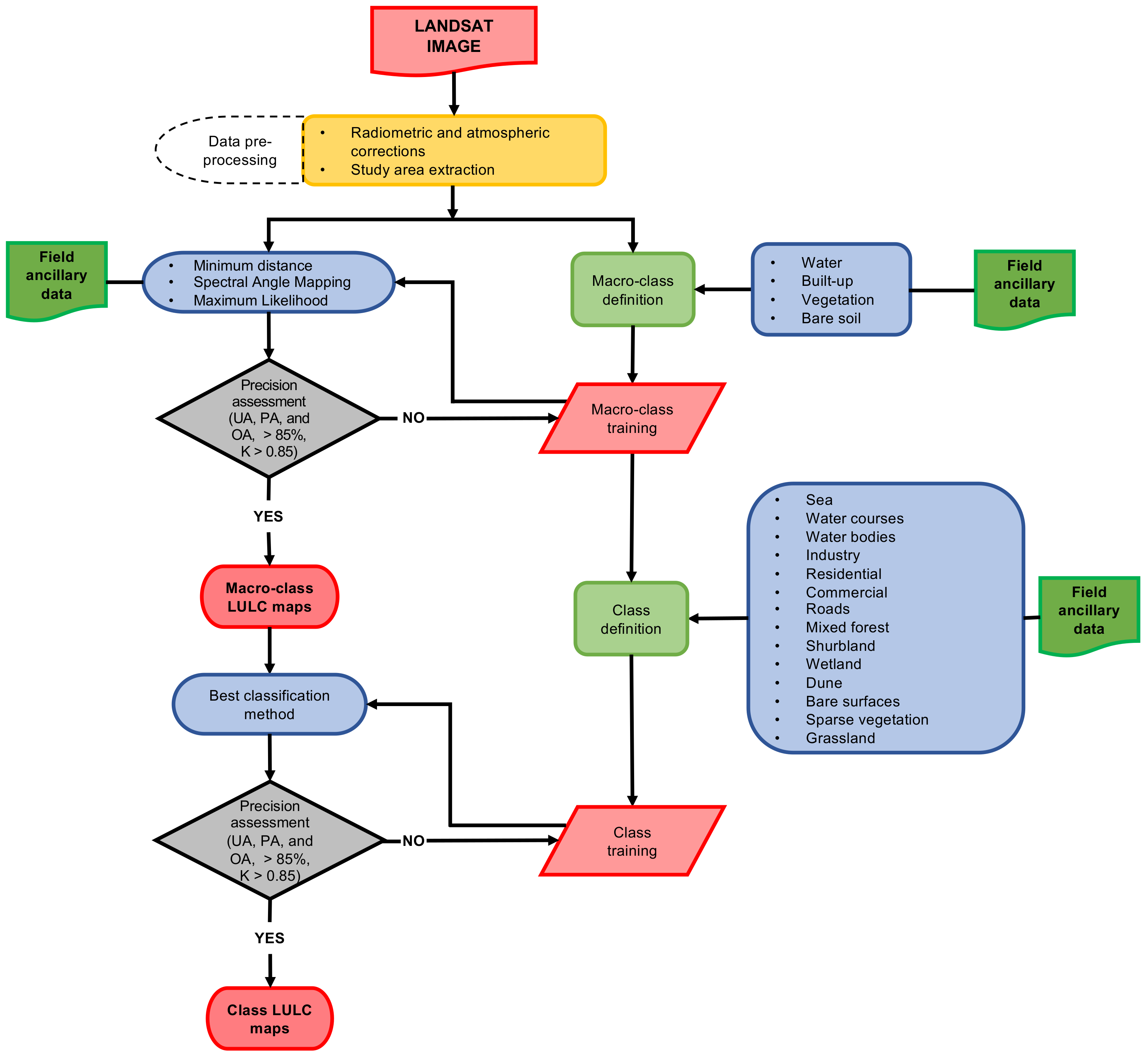
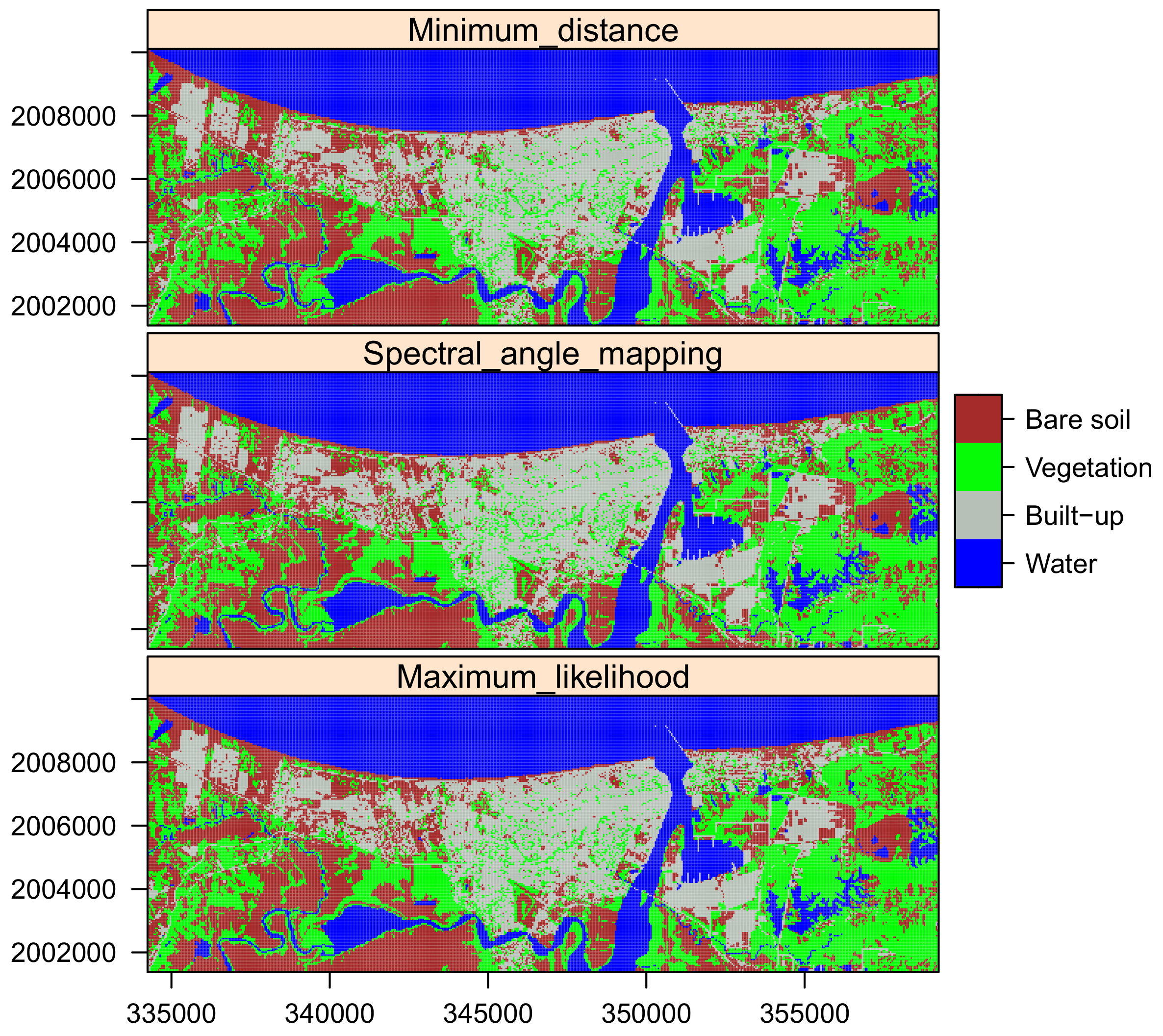
The three classification methods were run for the seven-year period proposed in this analysis. Results show a similar behavior for extracting LULC information using the same level of ancillary data. This condition allowed a fair comparison between the classification algorithms. Figure 3 shows the macro-class classification for the year 2017, which was the year which presented higher discrepancy among LULC classification methods. Graphically, one can observe that algorithms performed comparably. Significant variations were found within the clusters sharing bare soil and and built-up zones, whereas a more accurate definition was found for those composed of built-up vegetation and bare soil vegetation. These variations were attributed mostly to the spectral signature dispersion and departure within the pixels defining each class and the nearby areas. Bare soil and vegetation areas, being those mostly distributed over the west and east parts of the city, respectively, presented similar spatial distributions.

Numerically, all the classification methods presented good behavior for both overall precision and Kappa values, all being above 85% and 0.85, respectively (

Table 6. Precision assessment of the macro-class-based classification for 2017 under three classification methods.

	MDM		SAM		MLC
Year	OP	K	OP	K	OP	K
2015	89.12	0.85	88.89	0.85	93.28	0.91
2016	88.91	0.85	88.91	0.85	90.72	0.88
2017	89.31	0.86	89.28	0.86	95.36	0.94
2018	89.53	0.86	89.27	0.87	98.14	0.98
2019	90.13	0.87	89.90	0.86	90.02	0.87
2020	90.13	0.87	89.87	0.86	99.34	0.99
2021	89.67	0.86	89.43	0.86	96.95	0.96

). The spectral angle mapping (SAM) was the method that showed the smallest overall precision and Kappa values, 89% and 0.86, respectively. The highest accuracy was obtained using the maximum likelihood classifier (MLC), which presented overall precision above 90% and Kappa coefficients above 0.90 for all the years in the study period. It was observed that the MLC required less field data to obtain accuracy compared to the other classification methods.

The three classification methods showed the advantages of a perfect decision boundary to distinguish the macro-classes and a consistent mathematical expression based on the decision boundary for further classifications. However, these methods might overtrain the decision tree, as the training set needs several examples to cover all the possible cases within a specific class. Lastly, training tends to require significant computational time to be effective. As the MLC presented the highest level of accuracy under the same training set, it was selected as the main classification method for this study.

3.2. Macro-Class-Based LULC Classification

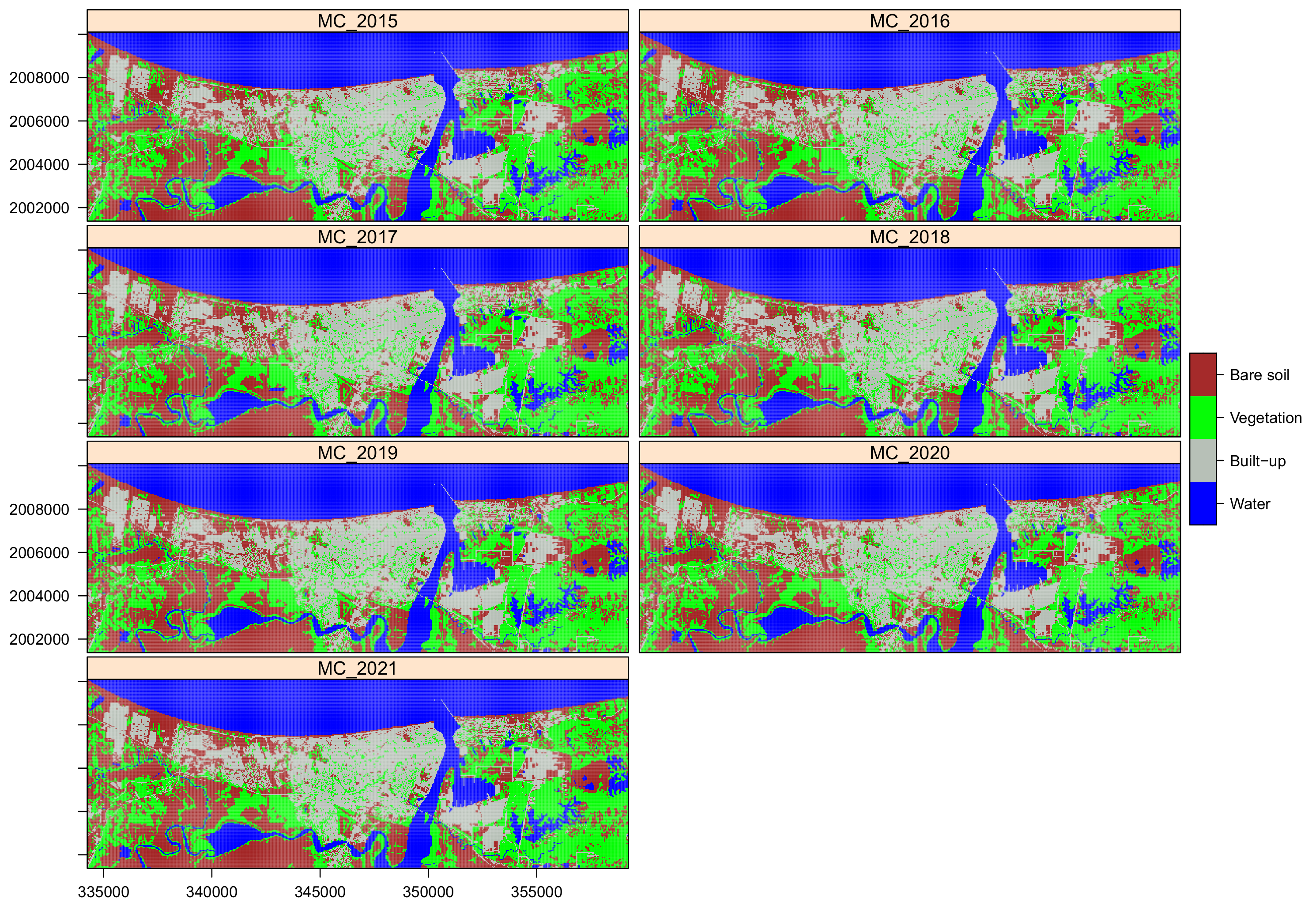
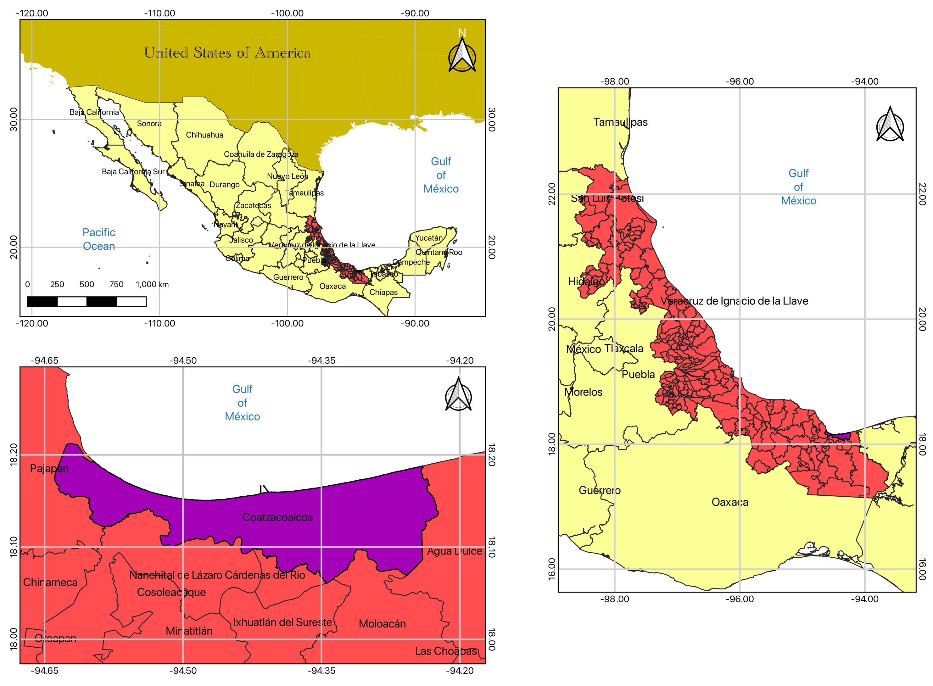
The classification based on macro-classes represented a course scheme to generate four of the main land uses found in Coatzacoalcos. These macro-classes are water, built-up, vegetation and bare soil. The spatial distribution of them can be observed in Figure 4. Graphically, one can see that the terrestrial surface is proportionally divided into three land uses without considering water. Most of the urbanization or built-up areas are in the north and south of the city near the river, as they were sites of the first settlers since the foundation of the city. However, the south potential flood areas and their development have been delayed, and small changes can be observed. It can also be seen that both north and south areas contain significant patches of vegetation, which, including the creation of green areas, is a good practice in urbanization development. However, urbanization in the west area of the city seemed to increment over the study period, but no vegetation buffers were observed in those zones. This indicates the absence of good practices in urbanization and government decisions in terms of territorial planning as well as the economic, social, cultural and environmental unconsciousness of new developers [70]. These zones may provoke a higher temperature sensation or heat islands, which might translate into health problems for the inhabitants [71]. Additionally, bare soil areas seemed to increase over time and were more prominent in the west area of the study. As seen in Figure 4, bare soil replaced areas of vegetation and also increased close to developed areas. These changes can be attributed to water availability during the growing season and afforestation during the development of urbanization.

In terms of vegetation, the east part of the city seemed to remain unaltered, except for zones near Allende Village in the northeastern and southeastern parts of the city, where the industries and petrochemical complexes are located and trigger the soil degradation. Numerically,

Table 7. Percentage area estimated for the macro-class-based classification.

Macro-Class	2015	2016	2017	2018	2019	2020	2021
Water	28.45	28.44	28.50	28.47	28.43	28.44	28.44
Built-up	19.88	19.92	19.99	20.03	20.12	20.15	20.21
Vegetation	26.00	25.98	25.74	25.56	25.46	25.18	24.96
Bare soil	25.67	25.66	25.77	25.94	25.99	26.24	26.37

supports the claim observed on the above maps. Pixels representing water show small variations attributed to possible changes in the surface water balance, but a more refined classification is needed to understand how these variations occurred. The maximum percentage of water land use was $28.58\%$ in 2017, whereas its minimum was $28.43\%$ in 2019. 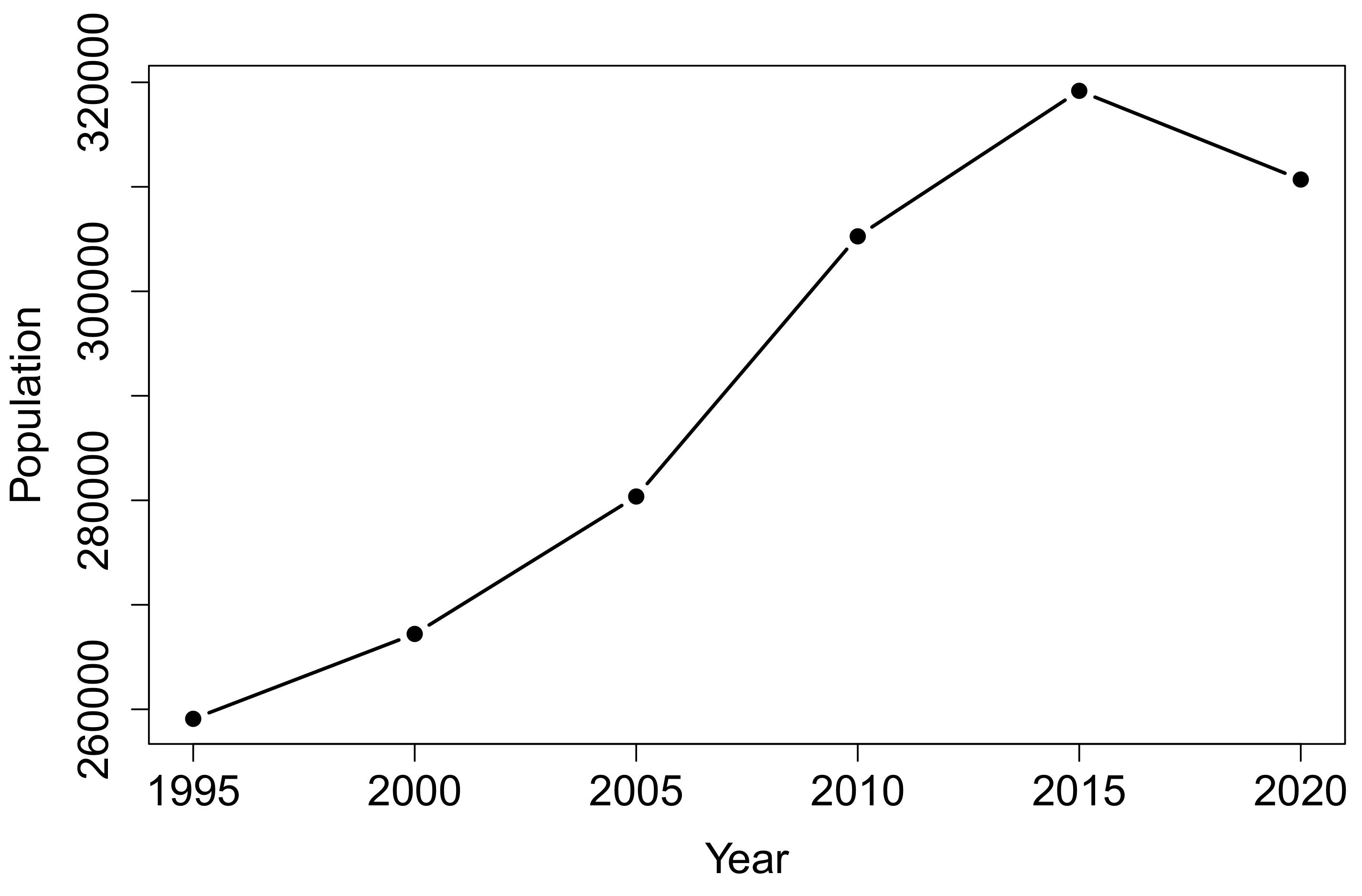Urbanization or man-made construction increased from $19.88\%$ in 2015 to $20.21\%$ in 2021. This increment can be explained by the trend observed in Figure 5, which shows the last six 5-year censuses. Coatzacoalcos had a mean population growth rate from 1995 to 2015 equal to 2.68%. However, we can observe that a rate equal −0.54% was shown in 2020. This means that population growth decreased in the last census. This variation can be illustrated with the reported built-up information, where man-made construction showed similar increments on a year-to-year basis. Nonetheless, the growth from 2019 to 2020 was its minimum, and no change was seen in 2021. This decrease in population and the variation within estimated in this study have socio-economic drivers. The city of Coatzalcoalcos was the second most dangerous city in 2019 [72]. This fact provoked serious economic and social issues due to extortion, racketeering and kidnapping. People moved to nearby cities to feel safe, and big companies closed their services; as a result, unemployment rate grew and investments in the city slowed down, which, in turn, decelerated urbanization and industry development.

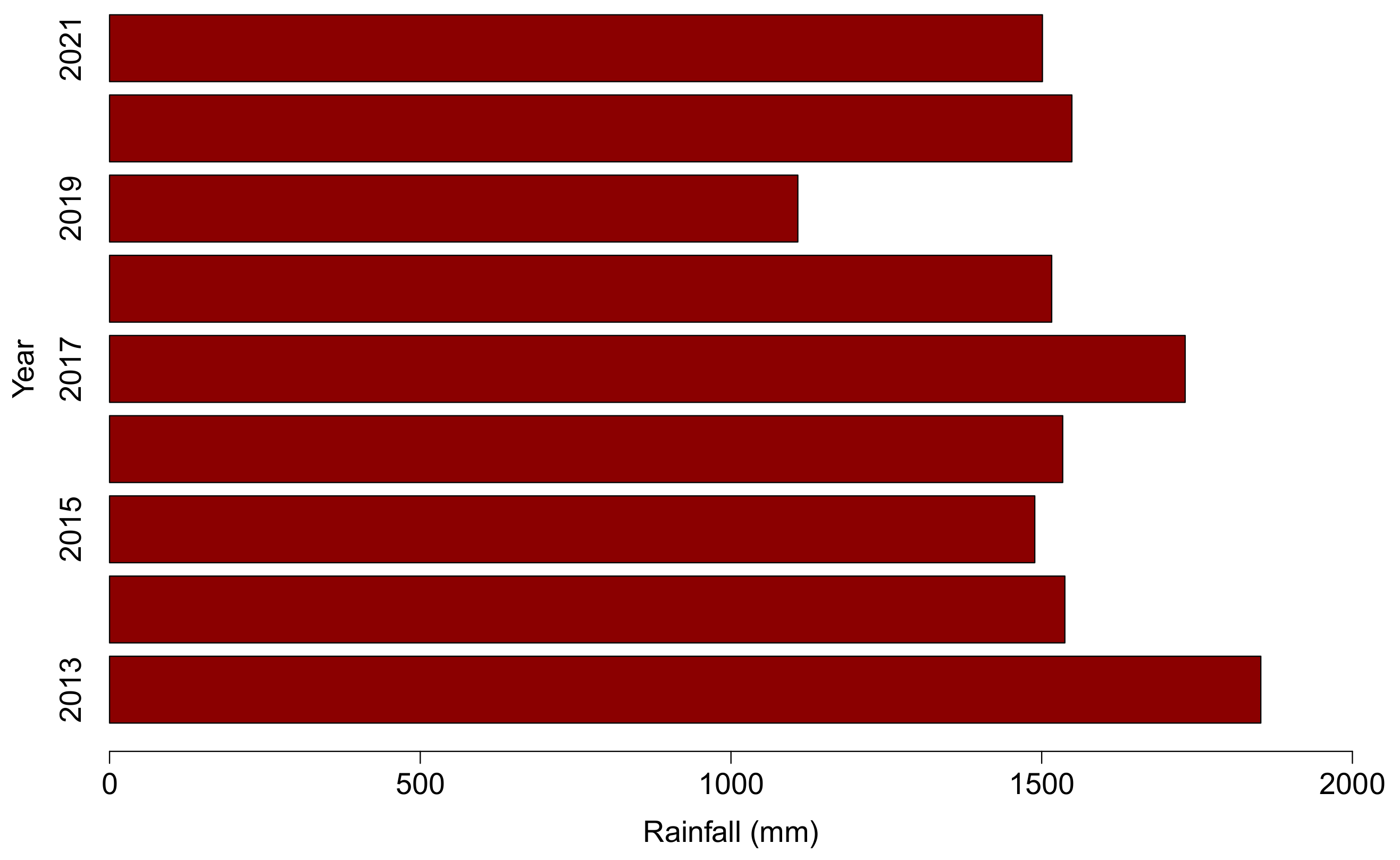
Bare soil also seems to increase visually in Figure 4 and is confirmed in Table 7. Bare soil variations are linked to a decrease in vegetation. These two variables are highly dependent on water availability, droughts and weather fluctuations. We can see that, in 2015, the area of study was 25.67% of bare soil, while, in 2021, it increased up to 26.37%. On the other hand, vegetation presented the inverse behavior, being 26% and 24.96% in 2015 and 2021, respectively. Analyzing the water availability, which is proportional to the precipitation, one can see in Figure 6 that rainfall tended to fluctuate from a minimum of 1107.6 mm in 2015 to a maximum of 1730.90 mm in 2017. This fluctuation, in general, tells us that, of the last three years of the period of analysis studied here, precipitation reduced drastically in 2019, which can explain the cause of the bare soil increment.

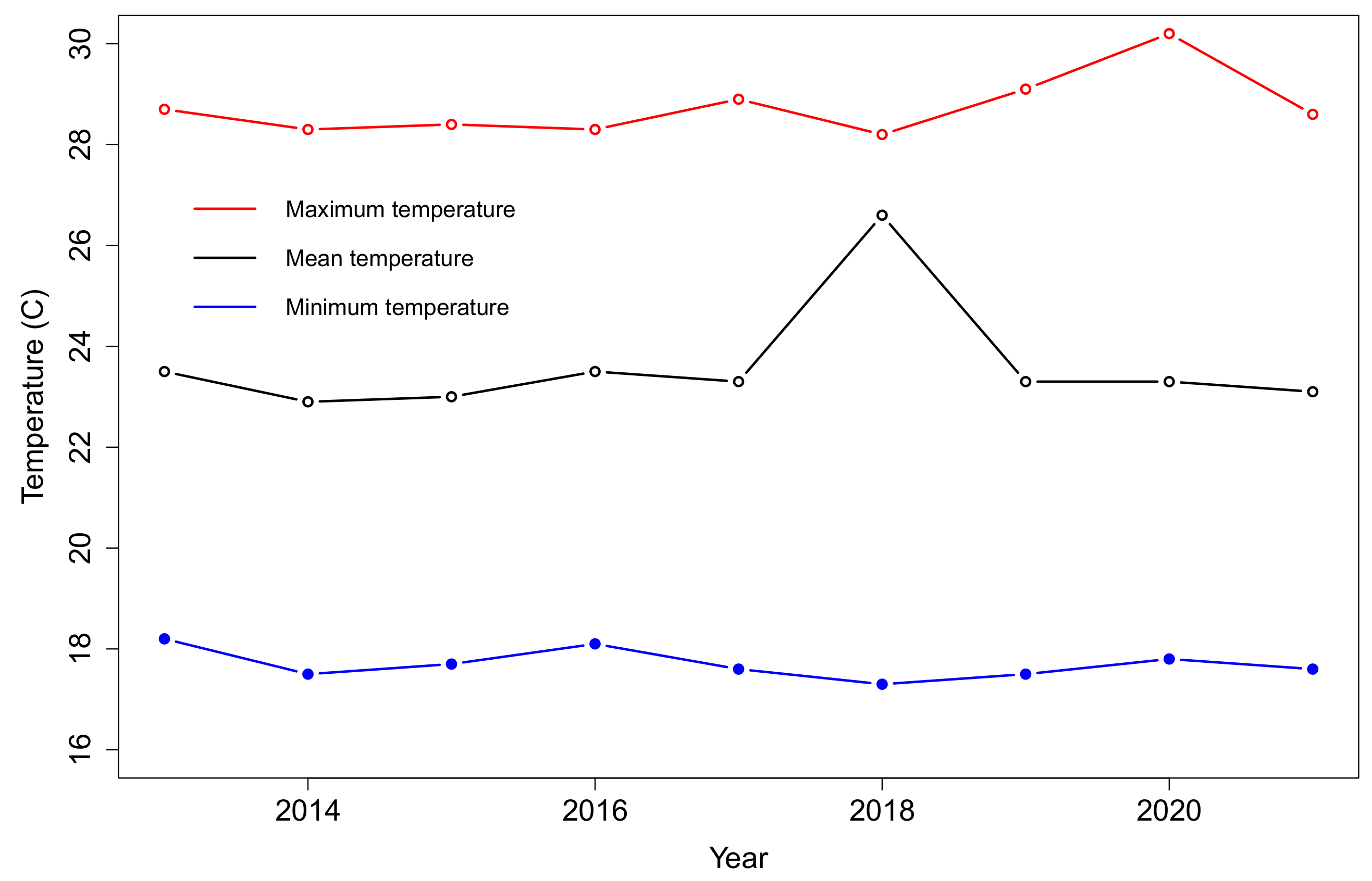
Additionally, Figure 7 shows that although minimum temperature tended to be steady from 2013 to 2021, mean temperature and maximum temperature increased during the study period. For instance, mean temperature was 26.60 ${}^{\circ }$C in 2018, whereas the maximum temperature increased from 28.20 to 30.20 ${}^{\circ }$C in 2018 and 2020, respectively. Increments in temperature increases soil evaporation and plant transpiration. If the latter is limited due to lack of water, water stress occurs in plants and they do not reach maturity, which might explain changes in pixel color and the move from vegetation to bare soil. It can be seen that the use of remote sensing for LULC evolution can be related and explained with inland information. This not only promotes the use of remote sensing but also validates its implementation. All the macro-class-based classification showed average user accuracy (UA) and producer accuracy (PA) higher than 90% (

Table 8. Overall precision and Kappa coefficient (K) for macro-class-based classification.

Measure	2015	2016	2017	2018	2019	2020	2021
UA	93.50	91.00	95.50	98.00	90.20	99.25	96.68
PA	93.06	91.45	96.04	98.06	90.32	99.36	96.60
Overall precision	93.38	90.72	95.36	98.14	90.02	99.34	96.75
K	0.91	0.88	0.94	0.98	0.87	0.99	0.96

).

This means that both producers and users of these maps can rely on this classification with at least 90% confidence. These values are comparable to the ones found in [47,48]. The mean overall precision for the study period is 94.81%. The Kappa coefficients for all the studied years are located in an excellent range, as they all are higher than 0.81, according to Viera and Garret [66]. Although this classification was appropriate for the proposed macro-classes, a more refined algorithm was implemented to understand more about the evolution of the LULC of Coatzacoalcos, as it is necessary for decision making purposes.

3.3. Class-Based LULC Classification

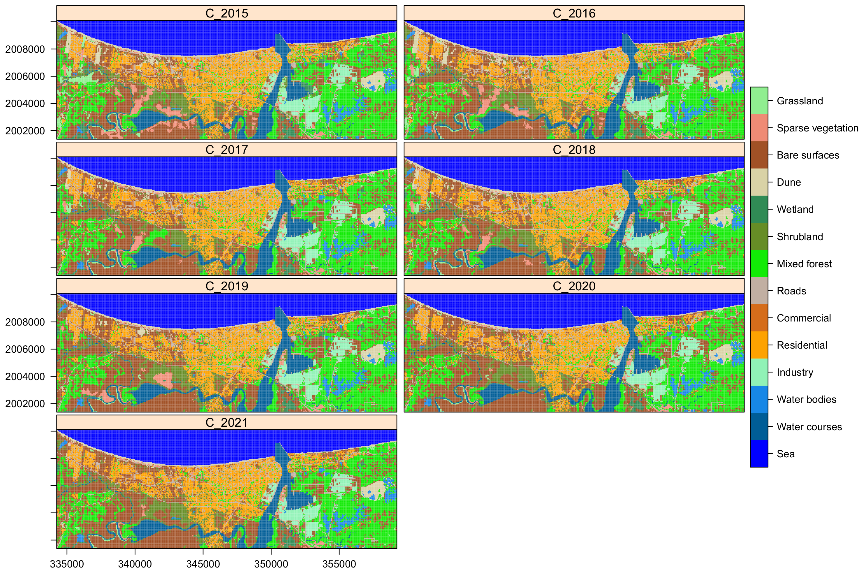
A class-based LULC classification was conducted to identify a more discrete evolution of the land use within the study period. This identification will help prioritize the location of areas that require ecological attention, the inclusion of best management practices (BMP) for water and soil conservation as well as a more appropriate location of the upcoming urbanization due to the Interoceanic Corridor project execution. At this level, we identified that pixels representing the sea did not change significantly. This behavior can be observed in Figure 8 and

Table 9. Percentage area estimated for the class-based classification.

Class	2015	2016	2017	2018	2019	2020	2021
Sea	20.10	20.1	20.1	20.09	20.1	20.1	20.1
Water courses	6.10	6.31	6.31	6.31	6.32	6.33	6.34
Water bodies	1.91	1.96	2.00	1.98	1.93	2.01	2.00
Industry	2.74	2.76	2.76	2.76	2.76	2.76	2.76
Residential	11.85	11.86	12.16	12.07	12.24	12.24	12.20
Commercial	0.52	0.51	0.46	0.55	0.45	0.44	0.50
Roads	4.77	4.78	4.84	4.84	4.81	4.83	4.87
Mixed forest	18.56	18.60	19.02	18.68	18.14	18.67	18.60
Shrubland	5.15	5.21	4.82	5.18	5.16	5.31	5.28
Wetland	1.86	1.40	1.10	1.13	1.13	0.93	0.92
Dune	2.83	2.79	2.28	2.30	2.15	1.96	1.96
Bare surfaces	19.31	20.71	22.12	22.02	22.61	23.19	23.20
Sparse vegetation	2.79	2.19	1.31	1.36	1.72	0.79	0.84
Grassland	1.51	0.81	0.64	0.66	0.41	0.41	0.42

, in which the percentage area representing the sea is about 20.1% for the entire period. However, water courses and water bodies seemed to change over time. Although these changes might not be significant, these changes can be confusing. We observed in Figure 6 that the annual precipitation throughout the study period decreased. As a result, bare soil area increased due to lack of water. One could assume that water bodies and water courses cannot increase in area. Nonetheless, this claim might not be entirely true, as increments of bare soil decrease infiltration and enhance the overland flow of the areas draining to the closest water courses. For that reason, water courses and water bodies in western areas increased due to increment of overland runoff in areas classified into bare soil with different vegetation densities (i.e., bare surfaces, sparse vegetation or grassland) and some over-flooded wetlands (i.e., swamps).

Man-made construction was divided into industry, residential, commercial and roads classes. Industry shows a constant percentage from 2016 to 2021. The only change occurred in 2015. The industrial area called Etileno XXI, the largest petrochemical complex in Latin America, concluded 99.2% of its construction in 2015 [75]. This, once again, confirms the accuracy of the generated map. Residence land use increased from 11.85% in 2015 to 12.24% in 2019 and maintained a steady value in 2021 (Table 9). This, once again, matches the period of violence described above that eventually provoked a decrease in population, as seen in Figure 5, which means that residence land use remained as it was in the previous years. Commercial areas showed fluctuations due to the city’s economical variation. It can be observed that, in 2018, commercial areas reached their maximum of 0.55%. However, the value decreased at the end of the study period (0.43%). A small increment was observed in 2021, when commercial areas increased to 0.50%. The city experienced transitions from high commercial zones to abandoned places due to the socio-economical problems previously described. These areas transformed either to low density vegetation areas or abandoned buildings. Lastly, in this class, roads were the most difficult to identify due to the Landsat satellite image resolution equaling 30 m. Roads close to the coast line and main avenues crossing from north to south and west to east were detected easily. However, narrow streets were not characterized as roads and they were either characterized as residence, commercial or industry classes. For that reason, although roads showed increments due to increase in population and urbanization development, no claim is expressed in order to avoid confusion in this class.

Vegetation plays an important role in our natural ecosystem and also holds up the biosphere in various ways. Vegetation helps to regulate the flow of numerous biogeochemical cycles, most importantly those of nitrogen, carbon and water. It also contributes to the local and global energy balances. In this study, the classes within vegetation included mixed forest, shrubland, wetland and dune. Figure 8 shows that mixed forest is the largest extension of the study area. One can see that the eastern and southwestern areas are dominated by this class, especially for those areas where no urbanization is present. Mixed forest occupied about 18% of city and its metropolitan area for the analyzed period, reaching its minimum in 2019 when the precipitation reached its lowest value (Figure 6). As previously mentioned, at this point, one can confirm that vegetation established in the urban areas were mostly mixed forest, having more pixels where the city was initially developed than where the more recent residential areas in the west of the city have been developed. Shrublands, in general, showed an increment over time. They reached their maximum percentage area, equal to 5.31%, in 2020 with some fluctuations in 2017, a year preceded by annual precipitation below 1500 mm, which represents the driest year of the analyzed period.

One of the most representative classes in this classification is wetland (i.e, swamps) because it represents multiple biological, economic and social values. Swamps provide services to ecological well-being, such as groundwater recharge, water purification, micro-climate regulation, food resources, biodiversity and carbon storage [76,77,78]. In the last decades, in Coatzacoalcos, urbanization has degraded swamps indiscriminately through industrial development or residential areas. These developments followed the erroneous idea that swamps were areas with dangerous species, such as snakes, alligators, mosquitoes, etc., which represented risks to the nearby areas [79]. This study evidences how wetland or swamp degradation continues. Visually, swamps located south and southeast of the city have mostly transitioned to some degree of vegetation density, either from water stress or landfill. In 2015, swamps represented about 2% of the study area, whereas, in 2021, this fraction reached 0.92%. This fact makes this study a good indicator to prevent and preserve swamps and wetlands within Coatzacoalcos and its metropolitan area due to the important ecological services that they represent.

Dunes, in Figure 8, are located along the coastline of the study area. In addition, there are some banks utilized by the industry (sandblasting) in the east area across the Coatzacoalcos river. One can see that dunes were replaced mainly by residential areas in the northwest part of the city. In 2015, dunes occupied almost 3% of the area in question. However, this area declined to 1.96% in 2021. The most significant evolution of urbanization occurred from 2017 to 2019. Additionally, the western coastline presented a transition from dunes to bare surfaces because that area is naturally preserved and the absence of tourism has improved the growth of native vegetation. Lastly, bare surfaces are the dominant land use along with mixed forest and residential areas (Figure 8). This land use increased from 19.31 to 23.19% through the study period in Table 9. Visually, most of the transitions were from sparse vegetation and high grassland to bare surfaces. This might have occurred because of the decrease in infiltration and precipitation previously mentioned and explored in Figure 6 and Figure 7. Sparse vegetation decreased from 2.79% to 0.79% and increased to 0.84% in 2021, whereas grasslands reduced from 1.51% to 0.42%.

Table A1. Precision assessment of the LULC maps of the city of Coatzacoalcos.

	2015			2016			2017			2018			2019			2020			2021
Class	UA	PA	K	UA	PA	K	UA	PA	K	UA	PA	K	UA	PA	K	UA	PA	K	UA	PA	K
Sea	100	99.86	1	100	100	1	100	100	1	100	98.72	1	100	100	1	100	100	1	100	100	1
Water courses	98	100	0.97	99	100	0.99	99	100	0.99	95.88	99.15	0.96	97	99.93	0.97	97	99.15	0.97	100	99.53	1
Water bodies	94.95	100	0.95	91.92	100	0.92	96.97	100	0.97	96	100	0.96	98	100	0.98	97.98	100	0.98	97.96	98.15	0.98
Industry	95.88	100	0.96	97	100	0.97	100	100	1	97.96	98.23	0.98	93.94	100	0.94	97	100	0.97	97.96	98.15	0.98
Residential	90	92.74	0.89	90	93.24	0.89	91	93.21	0.89	94	93.34	0.93	97	95.27	0.96	94	91.94	0.93	93	93.58	0.98
Commercial	94.84	80.48	0.95	95.24	100	0.95	95.88	100	0.96	96.81	100	0.97	97.96	91.02	0.98	98.97	100	0.99	97.89	93.41	0.98
Roads	100	86.49	1	96	86.41	0.96	95.96	86.71	0.96	96.97	88.32	0.97	99	90.09	0.99	94.95	86.95	0.95	97	83.78	0.97
Mixed forest	97	98.93	0.96	98	95.99	0.97	98	94.90	0.98	96	97.62	0.95	97	97.82	0.96	98	96.06	0.97	94	99	0.93
Shrubland	96	88.81	0.95	95	94.54	0.95	90.91	88.34	0.90	91	97.04	0.91	95	98.18	0.95	95	99.06	0.95	95	81.10	0.95
Wetland	98.98	91.39	0.99	96.84	100	0.97	98	100	0.98	98.97	96.54	0.98	100	94.72	1	97.92	99.06	0.98	96.91	98.07	0.97
Dune	99	100	0.99	98	99.28	0.98	96.94	98.22	0.97	99	100	0.99	96.94	98.18	0.97	98	95.44	0.98	98.98	88.96	0.98
Bare surfaces	93	95.80	0.91	96	97.19	0.95	94	97.29	0.92	99	98.50	0.98	97	98.76	0.96	96	98.57	0.95	91	97.14	0.89
Sparse vegetation	99	91.24	0.98	97.95	90.89	0.98	98.98	100	0.99	98.98	100	0.99	98.99	100	0.99	96.94	100	0.96	83.33	98.73	0.83
Grassland	94	96.49	0.94	94.90	100	0.95	94.85	100	0.95	98.93	95.90	0.98	94.85	100	0.95	93.75	100	0.94	94.62	100	0.95

shows the UA, PA and K values from each class throughout the analyzed period. User accuracy and producer accuracy show remarkable performance, with values within 90–100% and 80.48–100%, respectively. These individual accuracies, PA and UA, represent how well referenced pixels of the ground cover class are classified and the probability that a pixel classified into a given category actually represents that category on the ground, respectively. As expected, water and its classes showed the best performance, as it is the macro-class that presented the least variation while the other classes presented more significant variability. The Kappa coefficient shown for all classes was located in the range of excellent, according to the suggested values by Viera and Garret [66]. One can expect from these results that all the classes provide at least 90% confidence to the users of this information. The mean UA and PA values are presented in

Table 10. Overall precision and Kappa coefficient (K) for class-based classification.

Measure	2015	2016	2017	2018	2019	2020	2021
UA	96.48	96.13	96.46	97.11	97.33	96.82	95.13
PA	94.45	96.97	97.05	97.38	94.57	97.59	90.41
Overall precision	96.18	96.64	96.28	97.22	97.59	97.03	95.19
K	0.95	0.96	0.96	0.97	0.97	0.95	0.94

. Both UA and PA also are greater than 90%, as shown in each of the selected classes. The overall precision of the maps is also above 90%, which indicates that more than 90% of the reference pixels were correctly classified, and the K values validate the quality of this study, as they are all above 0.95.

3.4. Land Use and Land Cover Change through LULC Transition Matrix

The last part of the analysis of these results includes the generation of the LULC transition matrix (

Table A2. LULC matrix representing the class transitions. Units in km${}^2$.

Class	Sea	Water Courses	Water Bodies	Industry	Residential	Commercial	Roads	Mixed Forest	Shrubland	Wetland	Dune	Bare Surfaces	Sparse Vegetation	Grassland	Loss
Sea	43.85	0	0	0	0	0	0	0	0	0	0	0	0	0	0
Water courses	0	13.31	0	0	0	0	0.0009	0.0036	0	0.0009	0	0	0	0	−0.0054
Water bodies	0	0	4.13	0	0	0	0	0	0	0.0117	0	0.0009	0.0009	0	−0.0297
Industry	0	0	0	5.99	0	0	0	0	0	0	0	0	0	0	0
Residential	0	0	0	0	25.72	0.0909	0.0261	0	0	0	0	0.009	0	0	−0.126
Commercial	0	0	0	0	0.1449	0.95	0.0261	0.0009	0	0	0	0.0054	0	0	−0.1773
Roads	0	0	0	0.0027	0.0702	0.0216	10.30	0.0009	0	0	0	0.0108	0	0	−0.1062
Mixed forest	0	0	0.0009	0	0.0018	0.0009	0.0009	40.05	0.26	0	0	0.1188	0.0009	0.0432	−0.4383
Shrubland	0	0.0045	0.0063	0.0009	0.0261	0.0009	0	0.081	10.83	0	0	0.26	0.0261	0	−0.4095
Wetland	0	0.50	0.23	0	0	0	0.0063	0.31	0.29	1.97	0	0.7488	0.0117	0.0189	−2.0952
Dune	0.0189	0.0045	0	0.0135	0.31	0.0171	0.1575	0.0126	0.0324	0	4.26	1.323	0.0243	0.0063	−1.9206
Bare surfaces	0	0.0108	0.0081	0.0171	0.3087	0.0207	0.0468	0.0693	0.0135	0.0099	0.018	41.51	0.0756	0.0063	−0.6318
Sparse vegetation	0	0	0	0.0126	0.0081	0.0054	0.0306	0.0207	0.0288	0.0009	0	4.55	1.4319	0.0045	−4.6593
Grassland	0	0.009	0	0	0.0045	0.0009	0.0216	0.0279	0.0765	0.0072	0.0018	2.08	0.25	0.8046	−2.4795
Gain	0.0189	0.5238	0.2439	0.0486	0.882	0.1584	0.3159	0.522	0.6948	0.0306	0.0198	9.1179	0.396	0.1062	218.1617

), which indicates the transitions of each of the classes with respect to each other, for instance, how much area of the dunes converted to low vegetation density areas [69]. This matrix summarizes the changes already validated by the precision matrix but in terms of actual surface area. One disadvantage of this analysis is that it does not consider what happened throughout the two isolated years. However, it brings up an excellent tool for studies where LULC changes want to be predicted for future scenarios along with the possible drivers forcing those changes. The main diagonal contains the reference areas of the classes between the analyzed years. Columns named loss and gain represent the area lost or gained, respectively, for a particular class. Total gain or loss are calculated by adding up columns or rows of the reference area for each class. Particularly, this study selected the ends of the period, the years 2015 and 2021. The analysis of this matrix is straightforward. For instance, the water bodies gained 0.24 km${}^2$ but lost 0.0297 km${}^2$. Gains were associated with transitions of wetland (0.22 km${}^2$), shrubland (0.0063 km${}^2$), mixed forest (0.0009 km${}^2$) and bare surfaces (0.0081 km${}^2$) to water bodies. On the other hand, losses are due to a mixture of transitions, including sparse vegetation (0.009 km${}^2$), bare surfaces (0.009 km${}^2$) and wetlands (0.00117 km${}^2$). All these transitions occurred between the two selected classifications.

For the sake of simplicity, only the most significant changes are discussed here. Residential land use grew only 0.88 km${}^2$ during the last six years, which reflects a very small growth in comparison with that of industrial cities in Mexico, which has been characterized as about 5% per year [80], while Coatzacoalcos only grew 1% per year. Commercial areas reduced by 0.16 km${}^2$, resulting in abandoned areas due to the previous mentioned socio-economic issues. One of the prominent changes was in areas of mixed forest, which gained 0.52 km${}^2$ and lost 0.43 km${}^2$, indicating reforestation practices and more sustainable urbanization development in some new residential, industrial and commercial areas but some activities of deforestation. Swamps, on the other hand, lost 2.09 km${}^2$. This loss warns us of the possible future loss of ecological services provided by wetlands and their habitat, which are essential for biochemical processes and water purification because some of the non-point pollution in the city is contained by them. Lastly, vegetation densities fluctuated the most among them, namely, grassland and sparse vegetation density areas transitioned to bare surfaces. The latter gained 9.12 km${}^2$, whereas the former two lost 2.48 and 4.66 km${}^2$, respectively, which represents 80% of the bare surfaces gain.

4. Discussion

LULC changes measure the transitions of different land uses in complex interactions between humans and the physical environment [81,82]. Analysing LULC changes helps facilitate sustainable land use planning to protect and conserve the natural habitat and resources. The present study applied available remote sensing technology to classified course land uses, similarly to what has been presented in several studies [23,81,83,84,85,86]. The macro-classes identified were water, built-up, vegetation and bare soil. This first division allowed us to discriminate NDVI spectral indexes to improve a latter classification. Fractions of the area of study divided into macro-classes help us to observe the evolution of the city and its metropolitan area development and to explore the possible drivers forcing the changes in this initial classification. Broadly, some socio-economic factors, climate and topography were proposed as possible drivers. These drivers have also been identified as important factors for land use evolution [23,87,88,89]. This paper identified that security, precipitation, climate and topography were the main drivers causing LULC changes. Measurements such as producer accuracy (PA) and user accuracy (UA) showed high confidence, since they were higher than 90% for most of the macro-classes. These values are comparable and even superior to previous studies found in literature [49,84,89,90]. One can observe that the maximum likelihood classifier (MLC) is a suitable classification method to obtain acceptable results, as cited by several scientific contributions [34,35,58]. After the analysis of the macro-classes, 14 classes were exhaustively found to analyze and identify the land use in detail. Among those classes, some discussions are driven. Industry has experienced no change since the last petrochemical complex opened in 2015. Commercial areas have declined and residential zones present a slow increment due to the above-mentioned socio-economic drivers, which served to confirm the proposed hypothesis. Mixed forest and bare surfaces with low vegetation density tended to increase in surface area because reforestation programs and vegetation implemented in the coastline by the government have been a priority, as wind erosion has provoked much damage to the city’s infrastructure [91]. Swamps (i.e., wetlands) also showed an important decrease in spatial contribution, losing about 2 km${}^2$. This, in turn, might become an important environmental issue, since swamps are seen as important regulators of water pollution, carbon storage and habitat of species [92,93,94,95]. For that reason, actions need to be considered to avoid the continuous degradation of local wetlands and swamps. Additionally, it was observed that about 80% of the bare surface areas came from sparse vegetation and grassland areas. Associated changes in precipitation and high temperatures throughout the assessment period were responsible for these changes, as shown in results section. As a result of increments of bare surfaces, infiltration decreases and overland flow is exacerbated because soil properties such density, porosity and hydraulic conductivity depend on the level of established vegetation [96,97]. Lastly, a LULC transition matrix reflected the changes in surface area for each of the classes identified in this study. This is the baseline for future research that involves local problems in the city of Coatzacoalcos. A subsequent prediction of the land use using more extended spatial information of the drivers forcing the changes observed here will be proposed as an extension of this work. Additionally, the city is facing an issue with the relocation of solid residues, which naturally correlated with the actual land use. As a result, this study and methodology using higher-resolution imagery (i.e., sentinel satellite) help to study possible and suitable landfill sites.

5. Conclusions

This paper determined land use and land cover (LULC) over the period 2015–2021 for the city of Coatzacoalcos and its metropolitan area, located in the state of Veracruz, Mexico. Based on images from Landsat 8, MLC, Geographic Information Systems (GIS), NVDI spectral index and field data, the annual land use variability was produced up-to-date as reliable information for decision making and ecosystem preservation during the execution of the ongoing project called the Interoceanic Corridor. This project represents Mexico’s narrowest stretch between the Pacific and Atlantic oceans and the expansion and modernization of Coatzacoalcos and Salina Cruz ports.

The objective of this study was to provide the most recent information on land use spatial distribution that Coatzacoalcos experienced in the last six years and to improve the current available course resolution maps. The satisfactory results can be summarized in four main aspects: (1) built-up areas, including industry, residential and commercial areas, have slowed down their growth due to socio-economical drivers such as security and null monetary investments; (2) vegetation such as mixed forest and low density vegetation (bare surfaces, sparse vegetation and grassland) has been sustained and increased over time due to reforestation or migration from other classes; (3) swamps experienced considerable degradation over the past five years and (4) high and medium vegetation densities have transformed mostly to low vegetation densities due to climate drives such as low precipitation and possible high soil evaporation, which might also increase the overland flow for those areas.

Lastly, this study demonstrated the use of free available Landsat data and their processing by open source tools. It provided an accurate approach to mapping and assessing LULC changes over time. This methodology can be applied similarly for longer periods of time and other satellite products and contributes to improving the number of applications of remote sensing and research in Mexico and other developing countries.

References

1. Giri, C.; Wang, Y. Remote Sensing of Land Use and Land Cover; CRC Press: Boca Raton, FL, USA, 2012. [Google Scholar]
2. Gong, P.; Wang, J.; Yu, L.; Zhao, Y.; Zhao, Y.; Liang, L.; Niu, Z.; Huang, X.; Fu, H.; Liu, S.; et al. Finer resolution observation and monitoring of global land cover: First mapping results with Landsat TM and ETM+ data. Int. J. Remote Sens. 2013, 34, 2607–2654. [Google Scholar] [CrossRef] [Green Version]
3. Chowdhury, S.; Chao, D.K.; Shipman, T.C.; Wulder, M.A. Utilization of Landsat data to quantify land-use and land-cover changes related to oil and gas activities in West-Central Alberta from 2005 to 2013. GISci. Remote Sens. 2017, 54, 700–720. [Google Scholar] [CrossRef]
4. Ye, J.; Hu, Y.; Zhen, L.; Wang, H.; Zhang, Y. Analysis on Land-Use Change and Its Driving Mechanism in Xilingol, China, during 2000–2020 Using the Google Earth Engine. Remote Sens. 2021, 13, 5134. [Google Scholar] [CrossRef]
5. Muttitanon, W.; Tripathi, N.K. Land use/land cover changes in the coastal zone of Ban Don Bay, Thailand using Landsat 5 TM data. Int. J. Remote Sens. 2005, 26, 2311–2323. [Google Scholar] [CrossRef]
6. Gerard, F.; Petit, S.; Smith, G.; Thomson, A.; Brown, N.; Manchester, S.; Wadsworth, R.; Bugar, G.; Halada, L.; Bezak, P. Land cover change in Europe between 1950 and 2000 determined employing aerial photography. Prog. Phys. Geogr. 2010, 34, 183–205. [Google Scholar] [CrossRef] [Green Version]
7. Baumann, M.; Ozdogan, M.; Wolter, P.T.; Krylov, A.; Vladimirova, N.; Radeloff, V.C. Landsat remote sensing of forest windfall disturbance. Remote Sens. Environ. 2012, 143, 171–179. [Google Scholar] [CrossRef]
8. Clerici, N.; Paracchini, M.L.; Maes, J. Land-cover change dynamics and insights into ecosystem services in European stream riparian zones. Ecohydrol. Hydrobiol. 2014, 14, 107–120. [Google Scholar] [CrossRef]
9. Pervez, M.S.; Henebry, G.M. Assessing the impacts of climate and land use and land cover change on the freshwater availability in the Brahmaputra River basin. J. Hydrol. Reg. Stud. 2015, 3, 285–311. [Google Scholar] [CrossRef] [Green Version]
10. Balthazar, V.; Vanacker, V.; Molina, A.; Lambin, E.F. Impacts of forest cover change on ecosystem services in high Andean mountains. Ecol. Indic. 2015, 48, 63–75. [Google Scholar] [CrossRef]
11. Pasha, S.V.; Reddy, C.S.; Jha, C.S.; Rao, P.P.; Dadhwal, V.K. Assessment of land cover change hotspots in Gulf of Kachchh, India using multi-temporal remote sensing data and GIS. J. Indian Soc. Remote. Sens. 2016, 44, 905–913. [Google Scholar] [CrossRef]
12. Satyanarayana, B.; Thierry, B.; Seen, D.L.; Raman, A.V.; Muthusankar, G. Remote sensing in mangrove research-relationship between vegetation indices and dendrometric parameters: A case for Coringa, east coast of India. In Proceeding of the 22nd Asian Conference on Remote Sensing, Singapore, 5–9 November 2001; Volume 5, p. 9. [Google Scholar]
13. Liang, D.; Zuo, Y.; Huang, L.; Zhao, J.; Teng, L.; Yang, F. Evaluation of the consistency of MODIS Land Cover Product (MCD12Q1) based on Chinese 30 m GlobeLand30 datasets: A case study in Anhui Province, China. ISPRS Int. J. Geo-Inf. 2015, 4, 2519–2541. [Google Scholar] [CrossRef] [Green Version]
14. Randazzo, G.; Italiano, F.; Micallef, A.; Tomasello, A.; Cassetti, F.P.; Zammit, A.; D’Amico, S.; Saliba, O.; Cascio, M.; Cavallaro, F.; et al. WebGIS Implementation for Dynamic Mapping and Visualization of Coastal Geospatial Data: A Case Study of BESS Project. Appl. Sci. 2021, 11, 8233. [Google Scholar] [CrossRef]
15. Randazzo, G.; Cascio, M.; Fontana, M.; Gregorio, F.; Lanza, S.; Muzirafuti, A. Mapping of Sicilian Pocket Beaches Land Use/Land Cover with Sentinel-2 Imagery: A Case Study of Messina Province. Land 2021, 10, 678. [Google Scholar] [CrossRef]
16. Ghassemi, B.; Dujakovic, A.; Żółtak, M.; Immitzer, M.; Atzberger, C.; Vuolo, F. Designing a European-Wide Crop Type Mapping Approach Based on Machine Learning Algorithms Using LUCAS Field Survey and Sentinel-2 Data. Remote Sens. 2022, 14, 541. [Google Scholar] [CrossRef]
17. USGS. Available online: https://earthexplorer.usgs.gov (accessed on 10 December 2021).
18. Townshend, J.R.G.; Gayler, J.R.; Hardy, J.R.; Jackson, M.J.; Baker, J.R. Preliminary analysis of LANDSAT-4 Thematic Mapper. Int. J. Remote Sens. 1983, 4, 817–828. [Google Scholar] [CrossRef]
19. Lunetta, R.S.; Lyon, J.G.; Guindon, B.; Elvidge, C.D. North American landscape characterization dataset development and data fusion issues. Photogramm. Eng. Remote Sens. 1998, 64, 821–828. [Google Scholar]
20. Cohen, W.B.; Goward, S.N. Landsat’s role in ecological applications of remote sensing. Bioscience 2004, 54, 535–545. [Google Scholar] [CrossRef]
21. Taylor, P.; Horler, D.N.H.; Ahern, F.J. Forestry information content of Thematic Mapper data. Int. J. Remote Sens. 2007, 7, 37–41. [Google Scholar]
22. Campbell, J.B. Introduction to Remote Sensing, 4th ed.; The Guildford Press: New York, NY, USA, 2007. [Google Scholar]
23. Leta, M.K.; Demissie, T.A.; Tränckner, J. Modeling and Prediction of Land Use Land Cover Change Dynamics Based on Land Change Modeler (LCM) in Nashe Watershed, Upper Blue Nile Basin, Ethiopia. Sustainability 2021, 13, 3740. [Google Scholar] [CrossRef]
24. Pérez-Vega, A.; Mas, J.F.; Ligmann-Zielinska, A. Comparing two approaches to land use/cover change modeling and their implications for the assessment of biodiversity loss in a deciduous tropical forest. Environ. Model. Softw. 2012, 29, 11–23. [Google Scholar] [CrossRef]
25. Riad, P.; Graefe, S.; Hussein, H.; Buerkert, A. Landscape transformation processes in two large and two small cities in Egypt and Jordan over the last five decades using remote sensing data. Landsc. Urban Plan. 2020, 197, 103766. [Google Scholar] [CrossRef]
26. Tarasovicova, Z.; Saksa, M.; Blazik, T.; Faltan, V. Changes in agricultural land use in the context of ongoing transformational processes in Slovakia. Agriculture 2013, 59, 49–64. [Google Scholar]
27. Yuan, F.; Sawaya, K.E.; Loeffelholz, B.C.; Bauer, M.E. Land cover classification and change analysis of the Twin Cities (Minnesota) Metropolitan Area by multitemporal Landsat remote sensing. Remote Sens. Environ. 2005, 98, 317–328. [Google Scholar] [CrossRef]
28. Demissie, F.; Yeshitila, K.; Kindu, M.; Schneider, T. Land use/Land cover changes and their causes in Libokemkem District of South Gonder, Ethiopia. Remote Sens. Appl. Soc. Environ. 2017, 8, 224–230. [Google Scholar] [CrossRef]
29. Colditz, R.R.; Saldaña, G.L.; Maeda, P.; Espinoza, J.A.; Tovar, C.M.; Hernández, A.V.; Benítez, C.Z.; López, I.C.; Ressl, R. Generation and analysis of the 2005 land cover map for Mexico using 250 m MODIS data. Remote Sens. Environ. 2012, 123, 541–552. [Google Scholar] [CrossRef]
30. Blanco, P.D.; Colditz, R.R.; Saldaña, G.L.; Hardtke, L.A.; Llamas, R.M.; Mari, N.A.; Fischer, A.; Caride, C.; Aceñolaza, P.G.; del Valle, H.F.; et al. A land cover map of Latin America and the Caribbean in the framework of the SERENA project. Remote Sens. Environ. 2013, 132, 13–31. [Google Scholar] [CrossRef]
31. Morehart, C.T. Mapping ancient chinampa landscapes in the Basin of Mexico: A remote sensing and GIS approach. J. Archaeol. Sci. 2012, 39, 2541–2551. [Google Scholar] [CrossRef]
32. Robinson, C.J. Evolution of the 2014–2015 sea surface temperature warming in the central west coast of Baja California, Mexico, recorded by remote sensing. Geophys. Res. Lett. 2016, 43, 7066–7071. [Google Scholar] [CrossRef]
33. Alcalá, G.; Grisales-Noreña, L.F.; Hernandez-Escobedo, Q.; Muñoz-Criollo, J.J.; Revuelta-Acosta, J.D. SHP Assessment for a Run-of-River (RoR) Scheme Using a Rectangular Mesh Sweeping Approach (MSA) Based on GIS. Energies 2021, 14, 3095. [Google Scholar] [CrossRef]
34. Pal, M.; Mather, P.M. An assessment of the effectiveness of decision tree methods for land cover classification. Remote Sens. Environ. 2003, 86, 554–565. [Google Scholar] [CrossRef]
35. Osunmadewa, B.A.; Gebrehiwot, W.Z.; Csaplovics, E.; Adeofun, O.C. Spatio-temporal monitoring of vegetation phenology in the dry sub-humid region of Nigeria using time series of AVHRR NDVI and TAMSAT datasets. Open Geosci. 2018, 10, 1–11. [Google Scholar] [CrossRef]
36. Rawat, J.S.; Kumar, M. Monitoring land use/cover change using remote sensing and GIS techniques: A case study of Hawalbagh block, district Almora, Uttarakhand, India. Egypt. J. Remote. Sens. 2015, 18, 77–84. [Google Scholar] [CrossRef] [Green Version]
37. González-Mille, D.J.; Ilizaliturri-Hernández, C.A.; Espinosa-Reyes, G.; Costilla-Salazar, R.; Díaz-Barriga, F.; Ize-Lema, I.; Mejía-Saavedra, J. Exposure to persistent organic pollutants (POPs) and DNA damage as an indicator of environmental stress in fish of different feeding habits of Coatzacoalcos, Veracruz, Mexico. Ecotoxicology 2010, 19, 1238–1248. [Google Scholar] [CrossRef]
38. Morales, M.A.; Herrero, V.M.; Martinez, S.A.; Rodriguez, M.G.; Valdivieso, E.; Garcia, G.; Elias, M.A. Cleaner production and methodological proposal of eco-efficiency measurement in a Mexican petrochemical complex. Water Sci. Tech. 2006, 53, 11–16. [Google Scholar] [CrossRef]
39. BNAMERICAS. United States. 2021. Available online: https://www.bnamericas.com/en/features/mexicos-us1bn-interoceanic-corridor-to-start-operations-in-2023 (accessed on 10 December 2021).
40. INEGI. Available online: https://www.inegi.org.mx/temas/edafologia/ (accessed on 10 December 2021).
41. CONABIO. Available online: http://www.conabio.gob.mx/informacion/gis/ (accessed on 10 December 2021).
42. Prieto-Amparan, J.A.; Villarreal-Guerrero, F.; Martinez-Salvador, M.; Manjarrez-Domínguez, C.; Santellano-Estrada, E.; Pinedo-Alvarez, A. Atmospheric and radiometric correction algorithms for the multitemporal assessment of grasslands productivity. Remote Sens. 2018, 10, 219. [Google Scholar] [CrossRef] [Green Version]
43. Campbell, J.B. Evaluation of the dark-object subtraction technique for adjustment of multispectral remote-sensing data. In Digital Image Processing and Visual Communications Technologies in the Earth and Atmospheric Sciences II; International Society for Optics and Photonics: Bellingham, DC, USA, 1993; Volume 1819, pp. 176–188. [Google Scholar]
44. Chavez, P.S., Jr. An improved dark-object subtraction technique for atmospheric scattering correction of multispectral data. Remote Sens. Environ. 1988, 24, 459–479. [Google Scholar] [CrossRef]
45. Cui, Q.Y.; Gaillard, M.J.; Lemdahl, G.; Stenberg, L.; Sugita, S.; Zernova, G. Historical land-use and landscape change in southern Sweden and implications for present and future biodiversity. Ecol. Evol. 2014, 4, 3555–3570. [Google Scholar] [CrossRef]
46. Sobrino, J.A.; Jimenez-Munoz, J.C.; Paolini, L. Land surface temperature retrieval from LANDSAT TM 5. Remote Sens. Environ. 2004, 90, 434–440. [Google Scholar] [CrossRef]
47. El Hafyani, M.; Essahlaoui, A.; Fung-Loy, K.; Hubbart, J.A.; Van Rompaey, A. Assessment of Agricultural Water Requirements for Semi-Arid Areas: A Case Study of the Boufakrane River Watershed (Morocco). Appl. Sci. 2021, 11, 10379. [Google Scholar] [CrossRef]
48. Akbar, T.A.; Hassan, Q.K.; Ishaq, S.; Batool, M.; Butt, H.J.; Jabbar, H. Investigative spatial distribution and modelling of existing and future urban land changes and its impact on urbanization and economy. Remote Sens. 2019, 11, 105. [Google Scholar] [CrossRef] [Green Version]
49. Mohajane, M.; Essahlaoui, A.; Oudija, F.; Hafyani, M.E.; Hmaidi, A.E.; Ouali, A.E.; Teodoro, A.C. Land use/land cover (LULC) using landsat data series (MSS, TM, ETM+ and OLI) in Azrou Forest, in the Central Middle Atlas of Morocco. Environments 2018, 5, 131. [Google Scholar] [CrossRef] [Green Version]
50. Ding, Y.; Zheng, X.; Zhao, K.; Xin, X.; Liu, H. Quantifying the impact of NDVIsoil determination methods and NDVIsoil variability on the estimation of fractional vegetation cover in Northeast China. Remote Sens. 2016, 8, 29. [Google Scholar] [CrossRef] [Green Version]
51. Aburas, M.M.; Abdullah, S.H.; Ramli, M.F.; Ashaari, Z.H. Measuring land cover change in Seremban, Malaysia using NDVI index. Procedia Environ. Sci. 2015, 30, 238–243. [Google Scholar] [CrossRef] [Green Version]
52. Anim, D.O.; Kabo-bah, A.T.; Nkrumah, P.N.; Murava, R.T. Evaluation of NDVI using Spot-5 satellite data for northern Ghana. Environ. Manag. Sustain. Dev. 2013, 2, 167. [Google Scholar]
53. Song, C.; Woodcock, C.E.; Seto, K.C.; Lenney, M.P.; Macomber, S.A. Classification and change detection using Landsat TM data: When and how to correct atmospheric effects? Remote Sens. Environ. 2001, 75, 230–244. [Google Scholar] [CrossRef]
54. Richards, J.A. Remote Sensing Digital Image Analysis; Springer: Berlin, Germany, 1999. [Google Scholar]
55. Kosztra, B.; Büttner, G.; Hazeu, G.; Arnold, S. Updated CLC Illustrated Nomenclature Guidelines; European Environment Agency: Wien, Austria, 2017; pp. 1–124. [Google Scholar]
56. Richards, J.A.; Jia, X. Remote Sensing Digital Image Analysis: An Introduction; Springer: Berlin, Germany, 2006. [Google Scholar]
57. Kruse, F.A.; Lefkoff, A.B.; Boardman, J.W.; Heidebrecht, K.B.; Shapiro, A.T.; Barloon, P.J.; Goetz, A.F.H. The spectral image processing system (SIPS)—interactive visualization and analysis of imaging spectrometer data. Remote Sens. Environ. 1993, 44, 145–163. [Google Scholar] [CrossRef]
58. Currit, N. Development of a remotely sensed, historical land-cover change database for rural Chihuahua, Mexico. Int. J. Appl. Earth Obs. Geoinf. 2005, 7, 232–247. [Google Scholar] [CrossRef]
59. Otukei, J.R.; Blaschke, T. Land cover change assessment using decision trees, support vector machines and maximum likelihood classification algorithms. Int. J. Appl. Earth Obs. Geoinf. 2010, 12, S27–S31. [Google Scholar] [CrossRef]
60. Foody, G.M. Status of land cover classification accuracy assessment. Remote Sens. Environ. 2002, 80, 185–201. [Google Scholar] [CrossRef]
61. Smith, C.; Brown, N. Erdas Field Guide. Revised and Expanded, 5th ed.; eClass: Atlanta, GA, USA, 1999. [Google Scholar]
62. Thomlinson, J.R.; Bolstad, P.V.; Cohen, W.B. Coordinating methodologies for scaling landcover classifications from site-specific to global: Steps toward validating global map products. Remote Sens. Environ. 1999, 70, 16–28. [Google Scholar] [CrossRef]
63. Anderson, J.R. A Land Use and Land Cover Classification System for Use with Remote Sensor Data; US Government Printing Office: Washington, DC, USA, 1976; Volume 964. [Google Scholar]
64. Lu, D.; Weng, Q. A survey of image classification methods and techniques for improving classification performance. Int. J. Remote Sens. 2007, 28, 823–870. [Google Scholar] [CrossRef]
65. Congalton, R.G. A review of assessing the accuracy of classifications of remotely sensed data. Remote Sens. Environ. 1991, 37, 35–46. [Google Scholar] [CrossRef]
66. Viera, A.J.; Garrett, J.M. Understanding interobserver agreement: The kappa statistic. Fam. Med. 2005, 37, 360–363. [Google Scholar]
67. Congedo, L. Semi-Automatic Classification Plugin: A Python tool for the download and processing of remote sensing images in QGIS. J. Open Source Softw. 2021, 6, 3172. [Google Scholar] [CrossRef]
68. Alshari, E.A.; Gawali, B.W. Development of classification system for LULC using remote sensing and GIS. Global Transitions Proceedings 2021, 2, 8–17. [Google Scholar] [CrossRef]
69. Olofsson, P.; Foody, G.M.; Herold, M.; Stehman, S.V.; Woodcock, C.E.; Wulder, M.A. Good practices for estimating area and assessing accuracy of land change. Remote Sens. Environ. 2014, 148, 42–57. [Google Scholar] [CrossRef]
70. Casado-Izquierdo, J.M.; Sánchez-Salazar, M.T. Coatzacoalcos: Reestructuración urbana e inversión privada en una ciudad media mexicana. EURE (Santiago) 2013, 39, 91–116. [Google Scholar] [CrossRef]
71. Tan, J.; Zheng, Y.; Tang, X.; Guo, C.; Li, L.; Song, G.; Chen, H. The urban heat island and its impact on heat waves and human health in Shanghai. Int. J. Biometeorol. 2010, 54, 75–84. [Google Scholar] [CrossRef]
72. Diario de Xalapa. Mexico. 2019. Available online: https://www.diariodexalapa.com.mx/local/habitantes-viven-inseguros-coatzacoalcos-ciudad-segundo-lugar-3914790.html/ (accessed on 21 December 2021).
73. INEGI. Censos y Conteos de Población y Vivienda, 1995 a 2020. Encuesta Intercensal 2015. 2020. Available online: http://ceieg.veracruz.gob.mx/wp-content/uploads/sites/21/2021/06/COATZACOALCOS_2021.pdf (accessed on 10 December 2021).
74. CONAGUA. Sistema Metereológico Nacional. México. 2021. Available online: https://smn.conagua.gob.mx/es/climatologia/temperaturas-y-lluvias/resumenes-mensuales-de-temperaturas-y-lluvias/ (accessed on 21 December 2021).
75. Braskem Idesa. Historia. Available online: https://www.braskem.com.br/idesa/historia (accessed on 21 December 2021).
76. Brasil, M.C.O.; de Magalhães-Filho, R.; do Espírito-Santo, M.M.; Leite, M.E.; Veloso, M.D.D.M.; Falcão, L.A.D. Land-cover changes and drivers of palm swamp degradation in southeastern Brazil from 1984 to 2018. Appl. Geogr. 2021, 137, 102604. [Google Scholar] [CrossRef]
77. Quintas-Soriano, C.; Castro, A.J.; Castro, H.; García-Llorente, M. Impacts of land use change on ecosystem services and implications for human well-being in Spanish drylands. Land Use Policy 2016, 54, 534–548. [Google Scholar] [CrossRef]
78. Tiner, R.W.; Lang, M.W.; Klemas, V.V. Remote sensing of Wetlands: Applications and Advances; CRC Press: Boca Raton, FL, USA, 2015. [Google Scholar]
79. Toledo, A.; Vázquez-Botello, A.; Herzig. El Pantano: Una Riqueza Que se Destruye; de Ecodesarrollo, C., Toledo, A., Eds.; Centro de Ecodesarrollo: México, 1987. [Google Scholar]
80. Sobrino, J. Desempeño industrial en las principales ciudades de México, 1980–2003. Estud. DemográFicos Urbanos 2007, 22, 243–290. [Google Scholar] [CrossRef] [Green Version]
81. Nayak, P.M.; Byrne, M.L. Impact of land use land cover change on a sand dune ecosystem in Northwest Beach, Point Pelee National Park, Canada. J. Great Lakes Res. 2019, 45, 1047–1054. [Google Scholar] [CrossRef]
82. Pielke Sr, R.A.; Pitman, A.; Niyogi, D.; Mahmood, R.; McAlpine, C.; Hossain, F.; de Noblet, N. Land use/land cover changes and climate: Modeling analysis and observational evidence. Wiley Interdiscip. Rev. Clim. Chang. 2011, 2, 828–850. [Google Scholar] [CrossRef]
83. Liping, C.; Yujun, S.; Saeed, S. Monitoring and predicting land use and land cover changes using remote sensing and GIS techniques—A case study of a hilly area, Jiangle, China. PLoS ONE 2018, 13, e0200493. [Google Scholar] [CrossRef]
84. Yirsaw, E.; Wu, W.; Shi, X.; Temesgen, H.; Bekele, B. Land use/land cover change modeling and the prediction of subsequent changes in ecosystem service values in a coastal area of China, the Su-Xi-Chang Region. Sustainability 2017, 9, 1204. [Google Scholar] [CrossRef] [Green Version]
85. Mohan, M.; Kikegawa, Y.; Gurjar, B.R.; Bhati, S.; Kolli, N.R. Assessment of urban heat island effect for different land use–land cover from micrometeorological measurements and remote sensing data for megacity Delhi. Theor. Appl. Climatol. 2013, 112, 647–658. [Google Scholar] [CrossRef]
86. Huang, W.; Liu, H.; Luan, Q.; Jiang, Q.; Liu, J.; Liu, H. Detection and prediction of land use change in Beijing based on remote sensing and GIS. Int. Arch. Photogramm. Remote Sens. Spat. Inf. Sci 2008, 37, 75–82. [Google Scholar]
87. Sarif, M.O.; Gupta, R.D. Spatiotemporal mapping of Land Use/Land Cover dynamics using Remote Sensing and GIS approach: A case study of Prayagraj City, India (1988–2018). Environ. Dev. Sustain. 2021, 24, 888–920. [Google Scholar] [CrossRef]
88. Kolb, M.; Mas, J.F.; Galicia, L. Evaluating drivers of land-use change and transition potential models in a complex landscape in Southern Mexico. Int. J. Geogr. Inf. Syst. 2013, 27, 1804–1827. [Google Scholar] [CrossRef]
89. Serra, P.; Pons, X.; Saurí, D. Land-cover and land-use change in a Mediterranean landscape: A spatial analysis of driving forces integrating biophysical and human factors. Appl. Geogr. 2008, 28, 189–209. [Google Scholar] [CrossRef]
90. Martínez, S.; Mollicone, D. From land cover to land use: A methodology to assess land use from remote sensing data. Remote Sens. 2012, 4, 1024–1045. [Google Scholar] [CrossRef] [Green Version]
91. Universo. Sistema de noticias de la UV. Mexico. 2019. Available online: https://www.uv.mx/prensa/regiones/coatzacoalcos/uv-presenta-propuesta-para-minimizar-arribo-de-arena-en-malecon-de-coatzacoalcos/ (accessed on 21 December 2021).
92. Xiao, K.; Li, H.; Shananan, M.; Zhang, X.; Wang, X.; Zhang, Y.; Liu, H. Coastal water quality assessment and groundwater transport in a subtropical mangrove swamp in Daya Bay, China. Sci. Total Environ. 2019, 646, 1419–1432. [Google Scholar] [CrossRef]
93. Yule, C.M. Loss of biodiversity and ecosystem functioning in Indo-Malayan peat swamp forests. Biodivers. Conserv. 2010, 19, 393–409. [Google Scholar] [CrossRef]
94. Sabo, M.J.; Bryan, C.F.; Kelso, W.E.; Rutherford, D.A. Hydrology and aquatic habitat characteristics of a riverine swamp: I. Influence of flow on water temperature and chemistry. Regul. River 1999, 15, 505–523. [Google Scholar] [CrossRef]
95. Sabo, M.J.; Bryan, C.F.; Kelso, W.E.; Rutherford, D.A. Hydrology and aquatic habitat characteristics of a riverine swamp: II. Hydrology and the occurrence of chronic hypoxia. Regul. River 1999, 15, 525–544. [Google Scholar] [CrossRef]
96. Thompson, S.E.; Harman, C.J.; Heine, P.; Katul, G.G. Vegetation-infiltration relationships across climatic and soil type gradients. J. Geophys. Res. Biogeosci. 2010, 115. [Google Scholar] [CrossRef] [Green Version]
97. Perkins, K.S.; Stock, J.D.; Nimmo, J.R. Vegetation influences on infiltration in Hawaiian soils. Ecohydrology 2018, 11, e1973. [Google Scholar] [CrossRef]
Figure 1. Location of Coatzacoalcos city in Veracruz, Mexico.
Applsci 12 01882 g001
Figure 2. Flow diagram of the LULC classification methodology implemented in the SCP tool.
Applsci 12 01882 g002
Figure 3. Maps of the macro-class-based classification for three classification methods for 2017: Top: minimum distance. Middle: spectral angle mapping. Bottom: maximum likelihood. Units: meters. Projection: WGS84 / UTM Zone 15N.
Applsci 12 01882 g003
Figure 4. Maps of the macro-class-based classification for the study period (2015-2021). Units: meters. Projection: WGS84 / UTM Zone 15N.
Applsci 12 01882 g004
Figure 5. Last six five-year censuses in Coatzacoalcos, Veracruz. Source: National Institute of Statistics and Geography (INEGI) [73].
Applsci 12 01882 g005
Figure 6. Annual precipitation in Coatzacoalcos, Veracruz. Source: Comision Nacional del Agua (CONAGUA) [74].
Applsci 12 01882 g006
Figure 7. Annual precipitation in Coatzacoalcos, Veracruz. Source: Comision Nacional del Agua (CONAGUA) [74].
Applsci 12 01882 g007
Figure 8. Maps of the class-based classification for the study period (2015–2021). Units: meters. Projection: WGS84 / UTM Zone 15N.
Applsci 12 01882 g008