Abstract
The research object of this paper is a geogrid-reinforced embankment. Through numerical simulation and data monitoring, the characteristics of vertical displacement, horizontal displacement, vertical earth pressure, horizontal earth pressure, and internal force in a geogrid-reinforced embankment are studied. The results show that: (1) According to the analysis of monitoring data, the cumulative horizontal displacement decreases and the cumulative vertical displacement increases with time. Additionally, the cumulative vertical displacement is greater than the cumulative horizontal displacement. (2) The vertical pressure of the fill and tensile stress of the geogrid are largest at the center of the structure section, and the horizontal earth pressure is also largest on both sides of the structure. (3) The numerical simulation value and actual monitoring value of the project are compared with the design value. It is found that the tensile force, horizontal pressure, vertical pressure, horizontal displacement, and vertical displacement of the geogrid are less than the design value. The simulated characteristic value is greater than the actual monitored characteristic value. The research results provide a reference for the design of similar geogrid-reinforced embankments.
1. Introduction
Geogrids have good mechanical properties, a low price, light weight, and high strength, and can effectively improve the overall strength of soil. They are widely used in soil embankment and slope engineering [1]. They were first developed by the British Netion company in the 1980s [2], and can be divided into unidirectional, bidirectional, and multidirectional forms [3]. Many scholars have conducted research on the mechanical properties, reinforcement mechanisms, and stability of geogrid-reinforced soil [4,5,6,7,8,9,10,11].
Many scholars take reinforced soil retaining walls and slopes as research objects, using numerical simulation [10,12], the strength reduction method [13], the discrete element method, laboratory tests, and other methods to conduct research [14,15]. Peng Weiping studied reinforcement stress distribution in the process of reinforcement in slope filling by daubing epoxy resin strips on the surface of a model geogrid and pasting strain gauges [16]; they found that the bonding effect of epoxy resin strips was more stable than that of flexible 703 adhesive strips. Yan Fengxiang conducted direct shear friction tests on the interface between four kinds of construction residue with different grades and three kinds of grills [17], and found that the relationship between the interface friction stress and unit shear displacement of grid-construction residue can be expressed by a hyperbolic model. Yi Fu studied the interface friction characteristics between a geogrid and fillers with different particle sizes [18], and found that the maximum pulling force on the geogrid increased with increasing filler particle size and pulling rate. Liu Huabei et al. analyzed the internal force of the reinforcement of a geosynthetic-reinforced soil retaining wall. It was found that the active earth pressure coefficient and the method of limit equilibrium slope analysis were suitable for analyzing the internal force of the reinforcement in the strength limit state of the reinforced earth retaining wall [19]. Shen Huazhang proposed an analysis method to simulate the progressive failure process of a strain-softening slope by adopting the strain-softening constitutive model and vector sum method, and analyzed the progressive failure process of the slope [20].
Terzaghi previously proposed the concept of the progressive failure of soil slope stability [21]. In a study by Morgenstern et al., a clay with near-perfect particle parallelism was prepared by consolidating a slurried kaolin in a large oedometer. Shear box samples trimmed at various angles in relation to the compression direction revealed no significant differences in drained strength. [22]. Lade et al., through a true triaxial test, found that their soil sample has smooth peak failure [23]. Wanatowski et al. found, through experiments, that dense sand and medium-dense sand tended to form shear bands in their natural state, while loose sand did not form obvious shear bands in the test [24]. Hamed M et al., through a laboratory study on the tensile properties of a geogrid in a granular layer, found that embedding a geogrid in a sand gravel layer can significantly improve the uplift resistance of backfill [25]. When analyzing the stability of a retaining structure using the vertical strip partition method, the influence of the length of the reinforcement band on improving the stability of the slope is ignored. Therefore, Lo et al. and Shahgholi et al. proposed the horizontal strip partition method on this basis [26,27]. Based on a study of the location of a fracture line, the conclusion that the broken-line fracture surface of a reinforced slope passes through the toe of the slope was obtained [28,29,30].
At present, many scholars have studied slopes and embankments through experiments, numerical simulation, and theoretical analysis. The research content is singular, and there is no combination with actual projects. There is little research on the characteristics of geogrid-reinforced earth embankments on high and steep slopes under static load, which leads to unclear displacement, filling pressure, and stress characteristics in geogrid-reinforced earth embankments under static load. Therefore, through data monitoring and the establishment of a two-dimensional finite element model, the mechanical state of a high, steep, sloped, geogrid-reinforced earth embankment under static action is analyzed, and the structural stability and actual stress characteristics are obtained.
2. Materials and Methods
2.1. General Project Overview
Figure 1 shows a schematic diagram of the soil embankment. The high and steep slope of the geogrid-reinforced earth embankment is the bullet retaining wall of an anti-terrorism base. The slope material is mainly gabion mesh, and the slope body is filled with flexible geogrid and graded crushed stone soil. The length of the earth embankment with a 30 m filling height is 134.5 m, the length of the earth embankment with a 20 m filling height is 322.6 m, and the top widths are both 4 m. The slope ratio on both sides is 1:0.364, in which the 30 m soil embankment is filled in three stages, as shown in Figure 1a. The 20 m high soil embankment is filled in two stages, as shown in Figure 1b, and the step width is 2 m. The plan is shown in Figure 1c. The thickness of the filling soil is 0.5 m, and the bottom of the structure is on a bearing layer that meets the requirements. The bearing layer is filled with 1.5 m thick cement to stabilize the sand and gravel. The bottom of the foundation is located on a sand-and-pebble stratum with good bearing capacity.
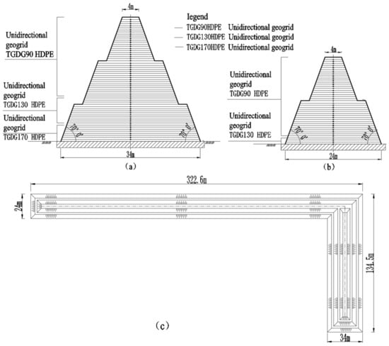
Figure 1.
Schematic diagram of soil embankment: (a) 30 m soil embankment; (b) 20 m soil embankment; (c) floor plan.
Figure 2 shows that the earth embankment transporting slope has not been removed yet. During construction, graded gravel soil is transported to the filling site for layering and rolling. One end of the earth-moving slope is in contact with the soil embankment. When the vehicle runs on the soil-moving pitch, the traffic load may cause the soil slope to move sideways, thus affecting the stability of the soil embankment. Therefore, in addition to real-time monitoring, the strength of the earth embankment is also appropriately increased. The form of the geogrid is shown in Figure 2.
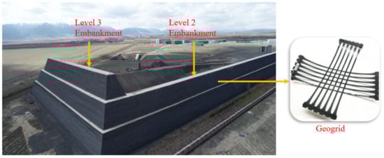
Figure 2.
Earth embankment.
2.2. Monitoring Content and Layout of Measuring Points
Figure 3 shows the comprehensive test instrument. The data-monitoring station records all data from the beginning to the end of construction. The monitoring data are composed of first-hand information on site, and can be used to accurately analyze the stress of the geogrid and fill, as well as the displacement and deformation of the structure. To monitor the tensile force of the geogrid, an intelligent digital flexible displacement meter with an observation accuracy of 0.01 mm is used, and a certain number of earth pressure boxes are buried to monitor the filling pressure. The comprehensive tester, with an observation accuracy of 600 Hz~3000 Hz, is used for data collection. After construction, an automatic complete testing system is used to continuously monitor the tension of the geogrid and the pressure change of the filling in real time. All the monitored data are extracted from the instrument.
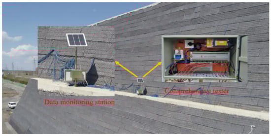
Figure 3.
Comprehensive tester.
2.3. Grid Force Monitoring
Figure 4 shows the cross-sectional layout of the monitoring elements of the 30 m high and 20 m high earth embankments, respectively. According to the analysis and calculation, we select the representative grid reinforcement layer, install a certain number of special flexible displacement meters to measure the tensile force of the geogrid, and master the distribution of the tensile stress of the geogrid along the length of the grid after construction is completed. The flexible displacement meters are, respectively arranged at the corresponding positions of the third-level earth embankment and the second-level earth embankment. The earth pressure boxes of the 30 m high earth embankment are set on the 9th, 20th, 30th, 39th, and 50th layers of the geogrid. The earth pressure boxes of the 20 m high earth embankment are set on the 9th, 20th, 30th, and 39th layers of the geogrid.
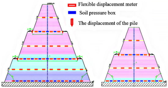
Figure 4.
Cross-section layout of monitoring elements for high soil embankment.
To monitor the change in earth pressure in the vertical and horizontal directions of the earth embankment, a certain number of steel-string earth pressure boxes are buried, and the earth pressure boxes for measuring the vertical earth pressure and the horizontal earth pressure are basically in the same position. The earth pressure boxes of the 30 m high earth embankment are arranged on the 9th, 20th, and 30th layers of the geogrid. The earth pressure boxes of the earth embankment with a height of 20 m are arranged on the 9th and 20th layers of the geogrid. They are arranged in the middle of two flexible displacement meters with a spacing of 3 m, symmetrically arranged from the middle to both sides, as shown in Figure 4. A certain number of displacement piles are buried on the slope toe and slope surface to observe the horizontal and vertical deformation of the slope and slope toe. According to the design data, the allowable vertical displacement is 0.007 m and the horizontal displacement is 0.006 m.
2.4. Displacement Monitoring
Figure 5 shows the arrangement of the displacement-monitoring points. An Independent coordinate system and elevation system are adopted for monitoring. When monitoring horizontal and vertical displacement, independent horizontal displacement and vertical displacement reference networks are set first. The horizontal displacement-monitoring reference network is measured using the polar coordinate method of the total station, and the vertical displacement-monitoring reference network is measured using the level. The actual vertical and horizontal displacement of the slope surface are observed according to the design requirements. The monitoring points are arranged on both sides of the slope surface. To simply and intuitively reflect the deformation characteristics, the datum point is set outside the influence range of engineering deformation, with good intervisibility conditions and a stable position. A total of 7 displacement observation reference points are set not far from the edge of the earth embankment, 32 monitoring points are set every 9 floors on the second-level earth embankment, and 17 monitoring points are set every 9 floors on the third-level earth embankment. The first- and second-level monitoring points of the third-level earth embankment and the second-level earth embankment are on the same floor, and the horizontal displacement reference points and the vertical displacement-monitoring reference points can be shared.
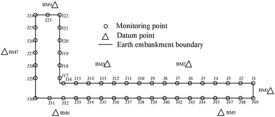
Figure 5.
Layout of monitoring points.
2.5. Model Building
Figure 6 shows the earth embankment and the earth embankment model. The simulation software used is Midas GTS NX 2018. All the monitoring points of the numerical simulation have been set in the model before the analysis. After the numerical analysis, the data of each monitoring point are extracted and analyzed (the monitoring points are A, B, C, D, E, F, and J in the following paragraphs). As the third-level steep-slope earth embankment is higher than the second-level earth embankment, and the geogrid and fill, in some parts, are more stressed, the third-level high steep-slope earth embankment is selected to establish the model. The two-dimensional model is established according to a ratio of 1:1 with the physical project. Figure 6a shows the entity of the third-grade earth embankment. The model is composed of four parts. The first part is the backfill layer of the graded sand gravel structure, including 60 layers at the third level and 40 layers at the second level. The thickness of each layer is 0.5 m. The second part is three types of geogrid with different tensile strengths: geogrids TGDG90 HDPE, TGDG130 HDPE, and TGDG170 HDPE. The third level is 60 layers of complete paving, and the second level is 40 layers of full paving. The spacing is 0.5 m. The third part is a 1.5 m water-stable replacement layer. The fourth part is the natural soil layer with a depth of 10 m. The mesh size of this model is about 0.5 m, and the mesh type is mixed mesh. The generated numerical model is shown in Figure 6b.
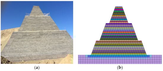
Figure 6.
(a) Third-grade soil embankment; (b) numerical model.
2.6. Setting Material Properties
The material parameters are reported through a geological survey project and obtained via large-scale triaxial test results of similar soil samples and geogrid complexes [31,32,33]. Layered rolling is required for filling. With the increase in filling height, the number of times rolling occurs when filling soil at the bottom gradually increases. Therefore, the actual strength parameter for filling soil at the construction site is larger than the experimental strength parameter, so it should be larger when setting the parameters. The material properties of the four parts are shown in Table 1.

Table 1.
Material property parameter table.
2.7. Establishing Contact Surfaces
The form of contact between the geogrid and fill is friction. Since the software program does not have an automatic contact function, it is necessary to establish contact units to fit. The contact unit is mainly a Goodman unit [34], which is mainly composed of c, φ, normal stiffness, and tangential stiffness. The tangential stiffness mainly simulates the friction slip between the geogrid and fill [35]. In the analysis, the normal stiffness value is large, and the default is such that the geogrid and fill cannot be embedded into each other. Table 2 shows the geogrid section and contact characteristic parameter table.
Table 2.
Geogrid section and contact characteristic parameter table.
2.8. Location Determination of Model Monitoring Points
Figure 7 shows the layout of the filling and geogrid monitoring points. To analyze and compare the filling pressure at different heights inside the structure, monitoring points C, B, and A are, respectively, set in the filling at the center line of the bottom layer of the first, second, and third levels, as shown in Figure 7a. To analyze and compare the plane stress of the filling at different heights inside and outside the structure, the first level, second level, and third level outside the bottom layer are selected, respectively, and the measuring points G, F, and E are set. As shown in Figure 7b, to analyze and compare the stress of the geogrid at different heights inside the structure, monitoring points J, I, and H are set on the geogrid at the center line of the bottom layer of the first, second, and third levels. The monitoring points of the numerical simulation are the same as the monitoring points set in the actual project.
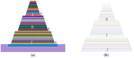
Figure 7.
(a) Schematic diagram of filling monitoring points; (b) geogrid monitoring points.
3. Monitoring Data Analysis
3.1. Analysis of Displacement-Monitoring Data
Figure 8(a-1–c-2) show the data of continuous daily monitoring at monitoring sites J1~J49 in the first, second, and third months, respectively. After completion of construction, horizontal and vertical displacements at each monitoring site were measured daily for 3 months. The single change value of each monitoring point is the average value of the 30-day monitoring value, the cumulative change value is the cumulative value of the 30-day monitoring value, and the rate of change is the ratio of the single change to the cumulative change value. It can be seen from the first displacement-monitoring dataset that the maximum single change value of horizontal displacement is close to 0.0055 m, and the maximum cumulative change value is about 0.004 m, with a relatively small change rate. The single change value and cumulative change value of different monitoring points differ greatly, which is caused by different compaction degrees in different parts of the same layer. From the vertical displacement, the difference between the maximum single change value and the cumulative change value is small, and the difference between the single change value and the cumulative change value of the two adjacent monitoring points is also small.
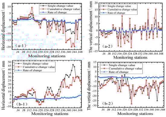
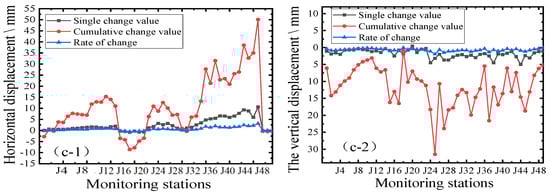
Figure 8.
Displacement-monitoring data: The first-month displacement-monitoring data ((a-1) horizontal displacement; (a-2) vertical displacement); the second-month displacement-monitoring data ((b-1) horizontal displacement; (b-2) vertical displacement); the third-month displacement-monitoring data ((c-1) horizontal displacement; (c-2) vertical displacement).
The displacement-monitoring data of the first month can be combined with that of the second and third months. The single change value decreases, and the cumulative change value is larger, the horizontal displacement of the cumulative value is smaller, and the vertical displacement of the total accumulative value increases. The single change value decreases, the cumulative change value increases, the cumulative value of horizontal displacement decreases, and the total cumulative value increases over time. The three change values in the first month are the largest, and the change values in the second months and third months decrease. This is because the horizontal fill of the remaining space is smaller, as under the action of gravity, the time needed for compaction is short, and the vertical space bigger, with most of the space under gravity populated. It takes a long time for the fill to be compacted again. After a comprehensive analysis, each displacement-monitoring value is within the allowable deformation range.
3.2. Analysis of Geogrid Monitoring Data
Figure 9 shows the tensile force of the geogrid. Figure 9(a-1,a-2), respectively, show the tensile force of the first group and the second group of geogrids. After the completion of construction, the data continuously observed by the flexible displacement meter, corresponding to the bottom layer of each level of the three-level earth embankment within one month, is selected to analyze the tensile force of the geogrid. First, we define the corresponding layer of each level. From top to bottom, the lowest layer of the third level is the first layer, the lowest layer of the second level is the second layer, and the lowest layer of the first level is the third layer. Then, representative earth embankments are selected for analysis. Because the third-level earth embankment and the second-grade earth embankment are similar in structure. The third-level earth embankment has greater analysis significance than the second-level earth embankment. Therefore, only the monitoring data of the Geogrid of the third-level earth embankments are analyzed, and the second-level earth embankments are not analyzed.
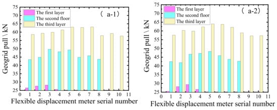
Figure 9.
Geogrid pull curve: (a-1) the first set of geogrid tension curves; (a-2) the second geogrid tension curve.
After construction, the gravity of the structure itself does not change. When the structure has small displacement, the soil particles acting on the flexible displacement meter slide, which cause displacement of the flexible displacement meter. From the 12 groups of continuous observation data, the data of each observation have little change. Two groups of data with obvious changes are selected to analyze the tensile force of the geogrid in the filling. The tensile forces of the two groups of geogrids obtained from the figure show that the tensile force of the geogrid in the center of the cross-section of the structure is the largest, and the tensile force of the geogrid on both sides is small. There are two reasons for this distribution. The first reason is that the tensile force is applied to the geogrid when the filling on both sides of the earth embankment is horizontally displaced. The second reason is that the vertical earth pressure is largest at the center of the embankment section.
3.3. Analysis of Earth Pressure-Monitoring Data
Figure 10 Shows vertical and horizontal earth pressure curves. Figure 10(a-1,a-2), respectively, show the first group of vertical earth pressure and horizontal earth pressure, and Figure 10(b-1,b-2), respectively, show the second group of vertical earth pressure and horizontal earth pressure. In order to obtain the distribution of vertical earth pressure, the data provided by two groups of earth pressure boxes are also selected for vertical and horizontal earth pressure analysis after construction. The buried position and layer of the selected earth pressure box is the layer of the flexible displacement meter. The first and second groups are also data that are continuously measured within one month after the completion of construction. According to the distribution of the earth pressure of the first, second, and third layers, the vertical earth pressure gradually decreases from the center of the structure section to both sides, indicating that the vertical earth pressure is largest at the center of the section of the earth embankment and the vertical earth pressure is smallest on both sides. This is because the structure section is symmetrical, and the gravity of the structure is the largest at the center of the structure section, so the vertical earth pressure on the center line is the largest.
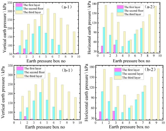
Figure 10.
Vertical and horizontal earth pressure curves: (a-1) the first group of vertical earth pressure; (a-2) the first group of horizontal earth pressure; (b-1) the second group of vertical earth pressure; (b-2) the second group of horizontal earth pressure.
The first group and the second group are two groups of data measured in the same period. From the distribution data of the two groups of horizontal earth pressure, the horizontal earth pressure of the earth embankment gradually increases from the center of the structural section to both sides. The horizontal earth pressure on both sides of the cross-section of the earth embankment is the largest, and the earth pressure is smallest at the center of the section. This is opposite to the distribution of vertical earth pressure.
3.4. Numerical Simulation of Displacement Analysis
The software analysis stage is the construction stage, and the original position is reset before the analysis. Because the thickness of the soil filling is 61 layers, the number of numerical simulation analyses is 61. After the numerical simulation analysis, the model is analyzed. Since the construction stage is not affected by time variables, data are obtained through the software extraction results. The location of extracted data in the model is basically the same as that of the actual monitoring point, and the extracted data are compared with the actual observation data.
Figure 11 shows vertical and horizontal displacement clouds. It can be seen from the vertical displacement cloud diagram in Figure 11a that the maximum vertical displacement is at the top of the structure. Because the vertical displacement of each layer of fill is accumulated under the gravity of the structure after construction, the maximum vertical displacement at the top is 0.0139 m, the middle vertical displacement is 0.0102 m, the minimum vertical displacement at the bottom is 0.0035 m, and the top vertical displacement is 0.046% of the wall height. It can be seen from the displacement cloud in Figure 11b that the horizontal displacement ranges from 0.0023 m at monitoring point G, 0.0017 m at monitoring point F, and 0.0016 m at monitoring point E due to the maximum lateral earth pressure and gravity at the bottom. It can be seen that the horizontal displacement is smaller than the vertical displacement.
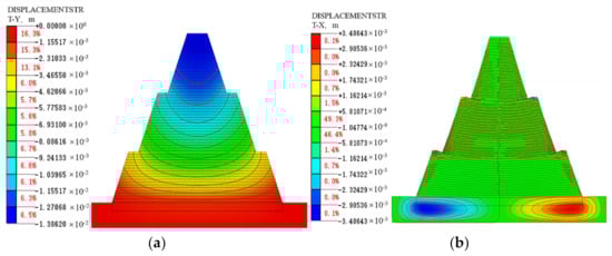
Figure 11.
Vertical and horizontal displacement cloud images: (a) vertical displacement cloud diagram; (b) horizontal displacement cloud diagram.
Figure 12 shows the horizontal and vertical displacement values of the simulation and actual monitoring. It is found that the measured vertical displacement and horizontal displacement are both greater than the measured monitoring displacement. This is because the actual engineering of the filled soil is anisotropic and heterogenous, and the fill in the numerical analysis is an ideal isotropic, uniform, numerical simulation of more accumulated disposable displacement. In general, the simulated displacement values are within the allowable displacement range [36]. From the point of view of numerical simulation, the displacement of the soil embankment on the same height of plane is basically close, and the left and right sides are basically symmetric, which is slightly different from the actual monitoring, but within the allowable range.
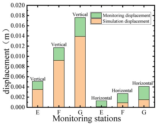
Figure 12.
Simulated vertical displacement values and actual vertical displacement-monitoring values.
3.5. Numerical Simulation of Fill Stress Analysis
Figure 13 shows vertical and horizontal earth pressure cloud diagrams. In Figure 13a, the plane stress values at monitoring points A, B, and C are 77.21 kPa, 203.84 kPa, and 305.15 kPa, respectively. The maximum plane stress of the traditional asymmetric reinforced soil slope is 2/3 h (H is the height of the soil bank), and the maximum earth pressure of the soil bank is found in the middle of the bottom of the structure in the cloud picture. Compared with the traditional asymmetric reinforced soil embankment, the embankment is most likely to be destroyed from the middle of the structure. As shown in Figure 13b, the horizontal earth pressure cloud map, the plane stress values of monitoring points E, F, and G are 59.71 kPa, 105.78 kPa, and 182.55 kPa, respectively. The main reason for horizontal plane stress is that the upper intermediate gravity compresses the filling on both sides.
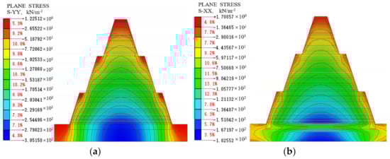
Figure 13.
Vertical and horizontal pressure cloud images: (a) vertical earth pressure cloud diagram; (b) horizontal earth pressure cloud diagram.
Figure 14 shows the vertical earth pressure and horizontal earth pressure of three monitoring points, A, B, and C, inside the embankment. In the figure, each measuring point, A, B, and C, has three values, respectively: the design’s allowable value, monitoring value, and numerical simulation value. It can be seen from the figure that the vertical earth pressure, horizontal earth pressure-monitoring value, and numerical simulation value of monitoring points A, B, and C do not exceed the design’s allowable vertical earth pressure and horizontal earth pressure. The ratios of the monitoring value, the simulated value, and the design’s allowed value of vertical soil pressure at points A, B, and C are 0.90, 0.90, 0.84, 0.84, 0.93, and 0.91, respectively. The ratios of the monitoring value, the simulated value, and the design’s allowable value of horizontal earth pressure at points A, B, and C are 0.77, 0.96, 0.97, 0.96, 0.85, and 0.89, respectively. Figure 14 further shows that the structure has good stability, and the vertical and horizontal stresses increase linearly from top to bottom along the internal central axis of the embankment.
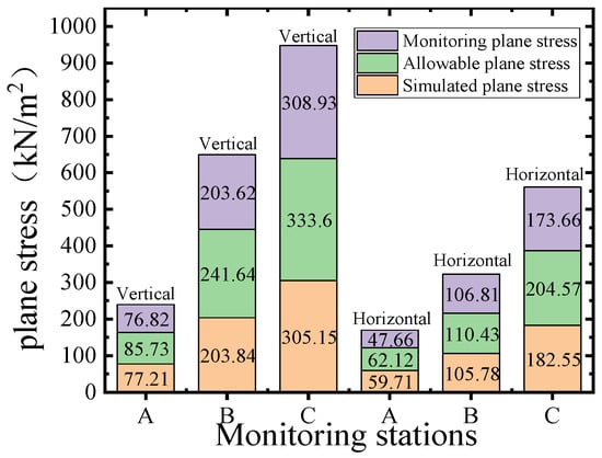
Figure 14.
Vertical and horizontal plane stresses.
3.6. Numerical Simulation of Geogrid Stress Analysis
Figure 15 shows a stress cloud diagram of the geogrid. The geogrid in the structure relies on the software to set the contact surface and the filling, and the stress between them is also transmitted by the set contact interface, so the internal force of the geogrid can be measured. After the construction, the working state of the geogrid has not reached the maximum. After the simulation, it can be seen from the cloud diagram that the internal force of the geogrid has reached the maximum value, and the stress increases from top to bottom, which is consistent with the actual monitoring of stress distribution.
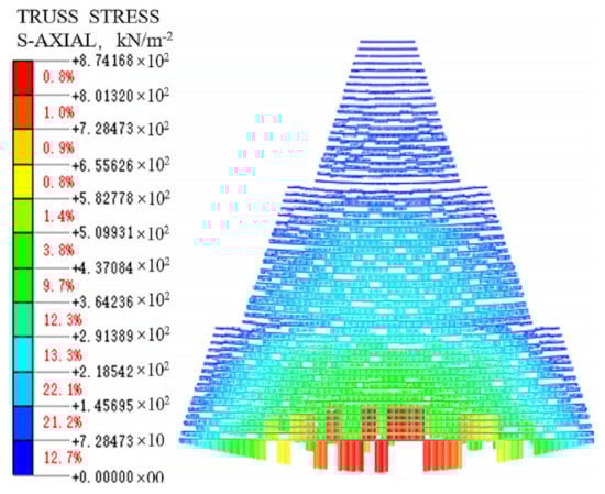
Figure 15.
Geogrid stress cloud.
It can be seen from the stress cloud in Figure 15 that the distribution of geogrid stress is consistent with that of filling pressure. The tensile stress levels of the geogrids at monitoring points H, I, and J are 72.84 kN/m2, 218.54 kN/m2, and 874.17 kN/m2, respectively. The long-term allowable tensile strengths are 18.2 kN/m, 26.5 kN/m, and 34.9 kN/m, respectively, as determined using the stress calculation formula. As can be seen from Figure 16 the simulated geogrid strength value at each measurement point is similar to the actual monitoring value, which is less than the long-term allowable tensile strength.
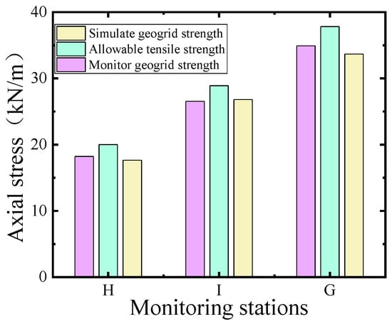
Figure 16.
Internal geogrid axial stress.
4. Conclusions
- (1)
- According to the analysis of monitoring data, the cumulative horizontal displacement of the geogrid-reinforced earth embankment decreases and the cumulative vertical displacement increases with time after construction. Additionally, the cumulative vertical displacement is greater than the cumulative horizontal displacement. Therefore, to prevent structural damage caused by excessive vertical displacement, the compactness of each layer of fill must be strictly controlled.
- (2)
- Through numerical simulation and data monitoring, it is found that the vertical pressure of the fill and the tensile stress of the geogrid are largest at the center of the structure section, and the horizontal earth pressure is largest on both sides of the structure. Therefore, in the design of similar structures in the future, the strength of the part where the structure bears the greatest force should be improved.
- (3)
- By comparing the monitored data and numerical simulation values, it is found that the tensile force of the geogrid, the horizontal pressure of the embankment fill, the vertical pressure, the horizontal displacement, and the vertical displacement are all less than the design values, indicating that the stability of the structure is good, and the geogrid inside the structure will not be broken.
Author Contributions
Conceptualization, Y.D. and J.C.; methodology, Y.D.; software, J.C.; validation, J.C. and J.L.; formal analysis, Y.D.; investigation, J.C.; resources, Y.D.; data curation, Y.D.; writing—original draft preparation, J.C.; writing—review and editing, J.C.; visualization, J.C.; supervision, Y.D.; project administration, J.L.; funding acquisition, Y.D. All authors have read and agreed to the published version of the manuscript.
Funding
This research received no external funding.
Informed Consent Statement
Informed consent was obtained from all subjects involved in the study.
Conflicts of Interest
The authors declare no conflict of interest.
References
- Dong, Y.L.; Han, J.; Bai, X.H. A numerical Study on Stress-Strain Responses of Biaxial Geogrids Under Tension at Different Directions. In Proceedings of the Advances in Analysis, Modeling & Design, GeoFlorida 2010; American Society of Civil Engineers: Reston, VA, USA, 2010; pp. 2551–2560. [Google Scholar] [CrossRef]
- Ghafoori, N.; Sharbaf, M. Evaluation of Triaxial Geogrids for Reduction of Base Thickness in Flexible Pavements. Bitum. Mix. Pavements 2015, VI, 141. [Google Scholar] [CrossRef]
- Al-Qadi, I.L.; Dessouky, S.; Tutumluer, E.; Kwon, J. Geogrid Mechanism in Low-Volume Flexible Pavements: Accelerated Testing of Full-scale Heavily Instrumented Pavement Sections. Int. J. Pavement Eng. 2011, 12, 121–135. [Google Scholar] [CrossRef]
- Abu-Farsakh, M.Y.; Chen, Q. Evaluation of Geogrid Base Reinforcement in Flexible Pavement Using Cyclic Plate Load Testing. Int. J. Pavement Eng. 2011, 12, 275–288. [Google Scholar] [CrossRef]
- Chen, Q.; Abu-Farsakh, M.; Tao, M. Laboratory Evaluation of Geogrid Base Reinforcement and Corresponding Instrumentation Program. Geotech. Test. J. 2009, 32, 516–525. [Google Scholar] [CrossRef]
- Xu, P.; Hatami, K.; Jiang, G. Seismic Sliding Stability Analysis of Reinforced Soil Retaining Walls. Geosynth. Int. 2019, 26, 485–496. [Google Scholar] [CrossRef]
- Gao, Y.; Yang, S.; Zhang, F.; Leshchinsky, B. Three-Dimensional Reinforced Slopes: Evaluation of Required Reinforcement Strength and Embedment Length Using Limit Analysis. Geotext. Geomembr. 2016, 44, 133–142. [Google Scholar] [CrossRef]
- Li, Z.-W.; Yang, X.-L. Stability Assessment of 3D Reinforced Soil Structures Under Steady Unsaturated Infiltration. Geotext. Geomembr. 2022, 50, 371–382. [Google Scholar] [CrossRef]
- Yang, K.H.; Nguyen, T.S.; Li, Y.H.; Leshchinsky, B. Performance and Design of Reinforced Slopes Considering Regional Hydrological Conditions. Geosynth. Int. 2019, 26, 451–473. [Google Scholar] [CrossRef]
- Duan, Y.F.; Song, L.; Liu, J.; Guo, M. Seismic Dynamic Response Analysis of Earth Embankment Reinforced with Geogrid on High Steep Slope. Sci. Technol. Highw. Transp. 2020, 37, 22–31. [Google Scholar]
- Esmaeili, M.; Naderi, B.; Neyestanaki, H.K.; Khodaverdian, A. Investigating the Effect of Geogrid on Stabilization of High Railway Embankments. Soils Found. 2018, 58, 319–332. [Google Scholar] [CrossRef]
- Tang, X.S.; Zheng, Y.R.; Wang, Y.F. Research on the Application of Double-Strength Reduction Method in Stability Analysis of Reinforced Soil Slope. Highw. Traffic Technol. 2018, 34, 14–17. [Google Scholar] [CrossRef]
- Chen, C.; Duan, Y.D.; Rui, R. Study on Strengthening Daoballast of Single and Double Geogrid Based on Pull-out Test and Discrete Element Simulation. Rock Soil Mech. 2021, 42, 954–962. [Google Scholar]
- Alotaibi, E.; Omar, M.; Shanableh, A.; Zeiada, W.; Fattah, M.Y.; Tahmaz, A.; Arab, M.G. Geogrid Bridging Over Existing Shallow Flexible PVC Buried Pipe–Experimental Study. Tunn. Undergr. Space Technol. 2021, 113, 103945. [Google Scholar] [CrossRef]
- Al-Rkaby, A.H.; Chegenizadeh, A.; Nikraz, H. Anisotropic Strength of Large-scale Geogrid-Reinforced. Sand: Experimental Study. Soils Found. 2017, 57, 557–574. [Google Scholar] [CrossRef]
- Peng, W.P.; Chen, L.W.; Liu, W.; Zhang, Q.H.; Li, C.A. Study on Strain Measurement Method of Model Geogrid. J. Hefei Univ. Technol. 2021, 44, 942–946. [Google Scholar]
- Yan, F.X.; Bai, X.H.; Dong, X.Q. Experimental Study on Friction Characteristics of Geogrid-construction Residue Interface. Rock Soil Mech. 2020, 41, 3939–3946. [Google Scholar]
- Yi, F.; Wang, Z.Y.; Du, C.B.; Zhang, Y. Experimental Study on Interaction Characteristics Between Geogratings and Fillers with Different Particle Sizes. Bull. Chin. Ceram. Soc. 2019, 38, 2557–2562. [Google Scholar]
- Liu, H.B.; Wang, L.; Wang, C.H.; Zhang, Y. Analysis of Internal Forces of Reinforced Soil Retaining Wall Reinforcement of Geosynthetics. Eng. Mech. 2017, 34, 1–11. [Google Scholar]
- Shen, H.Z. A Preliminary Study of the Progressive Failure and Stability of Slope with Strain-Softening Behavior. Rock Soil Mech. 2016, 37, 175–183. [Google Scholar] [CrossRef]
- Terzaghi, K. Soil Mechanics in Engineering Practice; Wiley: New York, NY, USA, 1996. [Google Scholar]
- Morgenstern, N.R.; Tchalenko, J.S. Microscopic Strictures in Kaolin Subjected to Direct Shear. Geotechnique 1967, 17, 309–328. [Google Scholar] [CrossRef]
- Lade, P.V.; Wang, Q. Analysis of Shear Banding in True Triaxial Test on Sand. J. Eng. Mech. 2001, 127, 762–766. [Google Scholar] [CrossRef]
- Suits, L.D.; Sheahan, T.; Wanatowski, D.; Chu, J. Stress-strain Behavior of a Granular Fill Measured by a New Plane Strain Apparatus. Geotech. Test. J. 2006, 29, 149–157. [Google Scholar] [CrossRef]
- Mirzaeifar, H.; Hatami, K.; Abdi, M.R. Pullout Testing and Particle Image Velocimetry (PIV) Analysis of Geogrid Reinforcement Embedded in Granular Drainage Layers. Geotext. Geomembr. 2022, 50, 1083–1109. [Google Scholar] [CrossRef]
- Lo, S.C.R.; Xu, D.W. A Strainbased Design Method For the Collapse Limit State of Reinforced Soil Walls and Slopes. Can. Geotech. J. 1992, 29, 832–842. [Google Scholar] [CrossRef]
- Shahgholi, M.; Fakher, A.; Jones, C.J.F.P.; Lam, J.; Li, K.S. Horizontal slice method of analysis. Géotechnique 2001, 52, 881–886. [Google Scholar] [CrossRef]
- Guler, E.; Enunlu, A.K. Investigation of Dynamic Behavior of Geosynthetic Reinforced Soil Retaining Structures Under Earthquake Loads. Bull. Earthq. Eng. 2009, 7, 737–777. [Google Scholar] [CrossRef]
- Magdii, M.E.E.; Richard, B.J. Experiment Design Instrumentation and Interpretation of Reinforced Soil Wall Response of Shaking Table. Phys. Model. Goetech. 2004, 4, 13–32. Available online: www.academia.edu/30942657 (accessed on 23 October 2022).
- Leshchinsky, D. Design Dilemma: Use Peak or Residual Strength of Soil. Geotext. Geomembr. 2001, 19, 111–125. [Google Scholar] [CrossRef]
- Liu, J. Experimental Study on Mechanical Properties and Reinforcement Mechanism of Geogrid-Reinforced Gravelly Soil. Hefei Univ. Technol. 2018, 6, 1–191. [Google Scholar]
- Coates, P.D.; Ward, I.M. The Plastic Deformation Behaviour of Linear Polyethylene and Polyoxymethylene. J. Mater. Sci. 1978, 13, 1957–1970. [Google Scholar] [CrossRef]
- Coates, P.D.; Ward, I.M. Neck Profiles in Drawn Linear Polyethylene. J. Mater. Sci. 1978, 15, 2897–2914. [Google Scholar] [CrossRef]
- Huang, D.L.; Tang, A.P.; Wang, Z.G. Analysis of Pipe-Soil Interactions Using Goodman Contact Element Under Seismic Action. Soil Dyn. Earthq. Eng. 2020, 139, 1062–1090. [Google Scholar] [CrossRef]
- Tran, V.D.H.; Meguid, M.A.; Chouinard, L.E. A Finite–Discrete Element Framework for the 3D Modeling of Geogrid–Soil Interaction Under Pullout Loading Conditions. Geotext. Geomembr. 2013, 37, 1–9. [Google Scholar] [CrossRef]
- Lalima, B.; Sowmiya, C.; Sujit, K. Application of Geocell Reinforced Coal Mine Overburden Waste as Subballast in Railway Tracks on Weak Subgrade. Constr. Build. Mater. 2020, 265, 120774. [Google Scholar] [CrossRef]
Publisher’s Note: MDPI stays neutral with regard to jurisdictional claims in published maps and institutional affiliations. |
© 2022 by the authors. Licensee MDPI, Basel, Switzerland. This article is an open access article distributed under the terms and conditions of the Creative Commons Attribution (CC BY) license (https://creativecommons.org/licenses/by/4.0/).