Abstract
In this paper, we adjust the hyperparameters of the training model based on the gradient estimation theory and optimize the structure of the model based on the loss function theory of Mask R-CNN convolutional network and propose a scheme to help a tennis picking robot to perform target recognition and improve the ability of the tennis picking robot to acquire and analyze image information. By collecting suitable image samples of tennis balls and training the image samples using Mask R-CNN convolutional network an algorithmic model dedicated to recognizing tennis balls is output; the final data of various loss functions after gradient descent are recorded, the iterative graph of the model is drawn, and the iterative process of the neural network at different iteration levels is observed; finally, this improved and optimized algorithm for recognizing tennis balls is compared with other algorithms for recognizing tennis balls and a comparison is made. The experimental results show that the improved algorithm based on Mask R-CNN recognizes tennis balls with 92% accuracy between iteration levels 30 and 35, which has higher accuracy and recognition distance compared with other tennis ball recognition algorithms, confirming the feasibility and applicability of the optimized algorithm in this paper.
1. Introduction
A national sport that evolved from traditional European aristocratic sports, tennis has become so popular worldwide for its unique spectacle and intense rivalry that it has overtaken basketball and volleyball as the second most popular sport in the world [1]. As tennis continues to grow, more and more people are joining the sport, resulting in many tennis stars and tennis enthusiasts. According to statistics, there are more than 10 million tennis fans and more than 100,000 tennis courts in China, growing at a rate of around 12% per year [2]. The number of people using tennis balls has increased dramatically, so it would take a lot of energy and time to pick up the tennis balls scattered around the court. Moreover, existing ball picking equipment cannot help reduce labor cost well. As a result, the use of robots to automatically identify and pick up tennis balls has become an increasingly popular demand [3,4].
Among them, there are various methods that can be applied to the autonomous recognition of tennis balls by robots, such as: direct recognition of the color and contour of tennis balls by the camera; and training of images of tennis balls using a cascade classifier on OpenCV. For example, in the literature [5] we relied on the color and contour classifier to recognize the target which is simple and efficient with less preparation, but only guarantees good recognition under ideal conditions such as stable camera operation, open field of view, no interference and clutter, good ambient light, etc., i.e., the anti-interference capability is not strong; then, in the literature [6] we relied on the cascade classifier to recognize the target which improved the anti-interference capability and detection efficiency, but recognition distance is shorter and requires more preparation work. Combining the advantages and disadvantages of the above methods, the deep learning method is chosen to train the image samples of tennis balls, which can ensure the anti-interference ability and recognize tennis balls at longer distances, and the recognition algorithm has strong robustness [7].
Based on deep learning, the corresponding neural network is designed and optimized to improve the recognition rate of the algorithm for tennis balls on outdoor places. For the problem of uneven lighting in outdoor places, the tennis ball image samples in different states are first collected, and then the sample data set is pre-processed [8]; for the problem of complex backgrounds and more people moving in outdoor places, the training data need to be correctly labeled. There exist many simple and effective neural networks for classifying targets and interferers in the input images using deep learning, for example, the improved Faster R-CNN is used in the literature [9] for target recognition, which improves the efficiency of target detection; however, its detection efficiency for small objects is low and there is an overfitting problem. Considering that the experiments described in this paper were conducted outdoors and the camera was moving most of the time, the Mask R-CNN convolutional network with one more mask branch for instance segmentation than the Faster R-CNN was chosen to optimize the recognition tennis algorithm. Mask R-CNN improves the convergence speed of the training model and saves training time by introducing weighted feature fusion of feature layers at different scales and improves the recognition efficiency of tennis balls as much as possible while ensuring the recognition accuracy of the algorithm for tennis balls [10].
In this paper, we design and optimize a deep learning algorithm system for tennis ball recognition that can be applied to intelligent tennis ball picking robots by referring to the literature of machine vision and computer vision. The rest of this paper is as follows: the basic composition and principles of deep neural networks are discussed in Section 2; the algorithmic model for robot recognition of tennis balls is designed and optimized in Section 3; the designed model is experimented and tested in Section 4; finally, the paper is concluded in Section 5.
2. Convolutional Neural Networks
Before discussing neural networks, it is important to clarify the basic idea of deep learning: a collection of algorithms for modeling highly complex data through multilayer nonlinear transformations [11]. As the basis of convolutional neural networks, artificial neural networks are complex networks composed of a large number of interconnected neurons with a high degree of nonlinearity, capable of performing complex logical operations and systems with nonlinear relational implementations [12]. Each neuron represents a specific output function called the activation function while the connection between every two neurons represents the weighted value of the signal passing through that connection, called the weight. Different weights and activation functions result in different outputs of the neural network.
As shown in Figure 1, the artificial neural network mainly consists of input layer (Input), output layer (Output), and hidden layer (Hidden). The i1, i2, and i3 in Figure 1 are the input layers, which are neurons receiving a large number of nonlinear input vectors (x1, x2, x3); the output layers o1 and o2 are the receiving units of the last layer to which the information flows after being transmitted, analyzed, and weighed in the link of the antecedent neurons, and are responsible for outputting the final result; the hidden layers are the neurons between the input and output layers with many neurons (h1, h2, h3, and h4) with weights wij constitute the various layers, which are the features of the input data abstracted to another dimensional space, thus better dividing the features linearly; if more than one hidden layer exists, it means there is more than one activation function whose ultimate purpose is to better linearly divide different types of data [13].
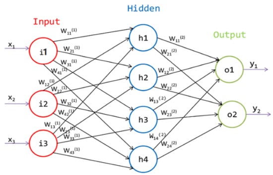
Figure 1.
Artificial neural network.
The convolutional neural network based on artificial neural network is a deep neural network with convolutional structure [14], which acts as a neural structure for multilayer supervised learning, uses gradient descent to minimize the loss function, and adjusts the weight parameters in the network in reverse layer by layer to improve the accuracy of the network. Convolutional neural network can better adapt to the feature structure of the image, which helps feature extraction and classification. The sharing of weights can reduce the training parameters of the network and make the neural network structure simple and applicable. As shown in Figure 2, the convolutional neural network mainly consists of an input layer, a convolutional layer, a pooling layer, a fully connected layer, and a Softmax layer [15].
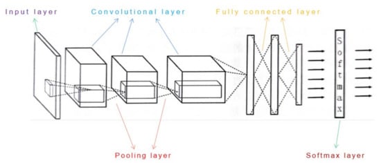
Figure 2.
Convolutional neural networks.
3. Experimental Method of Recognition Algorithm
This section is divided into three parts. In the first part, we briefly describe the experiments on tennis ball recognition based on color-and-contour-based traditional recognition algorithms. In the second part, we also briefly describe the experiments on tennis ball recognition based on cascade classifier. Finally, we focus on the experiments of Mask R-CNN convolutional network-based recognition algorithm for tennis balls.
3.1. Recognize Tennis Balls Based on Color and Contour Classifier
The robot identifies and segments pixels on the image that match the color characteristics of the tennis ball by a recognition algorithm based on the HSV color space and displays the tennis ball by a Hough circle transformation that distinguishes the pixels of the round contour object from other pixels on the image [16,17]. Among them, Figure 3 shows the color space distribution of HSV; Figure 4 shows the recognition algorithm detecting the image boundary of the tennis ball and drawing it as a circular contour (red circle in Figure 4) by using the Hough circle function, thus drawing the center of the circle of the contour by the radius (blue arrow in Figure 4) and outputting its pixel coordinates (a, b in Figure 4). In conclusion, under certain conditions, the robot can simply identify tennis balls by color and contour.
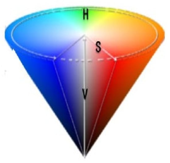
Figure 3.
HSV color space.
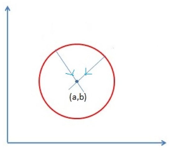
Figure 4.
Hoff gradient method to detect round.
Figure 5 shows the identification of tennis balls by color.
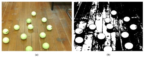
Figure 5.
HSV color space-based recognition of tennis balls. (a) Original image; (b) recognition effect picture.
Figure 6 shows the identification of tennis balls by contour.
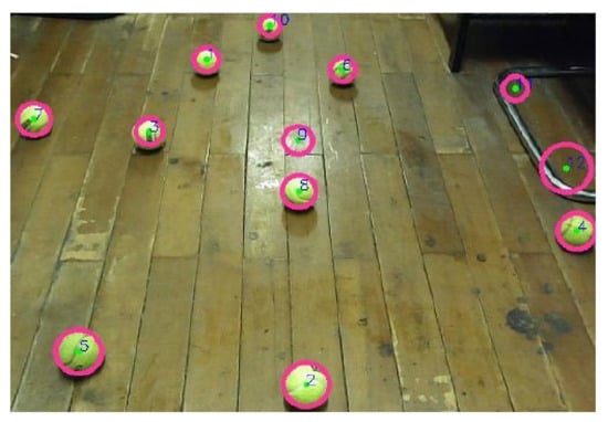
Figure 6.
Hoff circle gradient method for detecting tennis balls.
Figure 6 shows that after the tennis balls are detected using the Hoff circle gradient method, the recognition algorithm marks the number on each recognized tennis ball image for the researchers’ observation in order to count the number of tennis balls. In this case, the locations labeled with numbers 11 and 12 in Figure 6 are incorrectly drawn with circular outlines, which is a limitation of the Hough circle detection method that incorrectly identifies some clutter as tennis balls.
The robot recognizes tennis balls by the algorithm of color and contour features, which can only guarantee a good recognition effect under the ideal conditions of stable camera operation, open field of view, no interference and clutter, good ambient light, etc. If the background color is similar to the tennis ball color, the recognition effect is not obvious; secondly, the use of contour recognition tennis ball may identify some irrelevant items in the background.
3.2. Cascade Classifier-Based Recognition of Tennis Balls
Cascade classifier as an object detection method cleverly uses the Boosting algorithm, which is very good at detecting rigid objects from a specific viewpoint, and is a method to improve the accuracy of the algorithm by learning multiple times, boosting weak classifiers to strong classifiers, and iterating by providing weights to the training samples in each round of learning to finally reach a predetermined, sufficiently small error rate [18].
The cascade classifier is used to generate its own object classifier, firstly, positive and negative samples of tennis balls are collected (the tennis balls occupy the main pixel part in the images of positive samples, while the images of negative samples do not contain tennis balls), as shown in Figure 7 for the positive and negative samples of tennis balls collected in this paper; then the sample images are grayed out and normalized, using two executable files under opencv, opencv_ createsamples.exe and opencv_traincascade.exe to generate the image description file, that is, the positive and negative training samples; finally, enter the command in the terminal, set the corresponding parameters for training, and generate the training file.
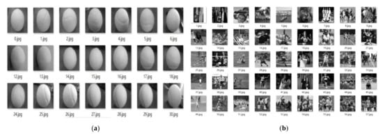
Figure 7.
Positive and negative sample description files. (a) Positive Sample, (b) negative sample.
As shown in Figure 8, the camera is turned on to acquire the image, and the trained detection model can be used to identify the tennis balls in the image.
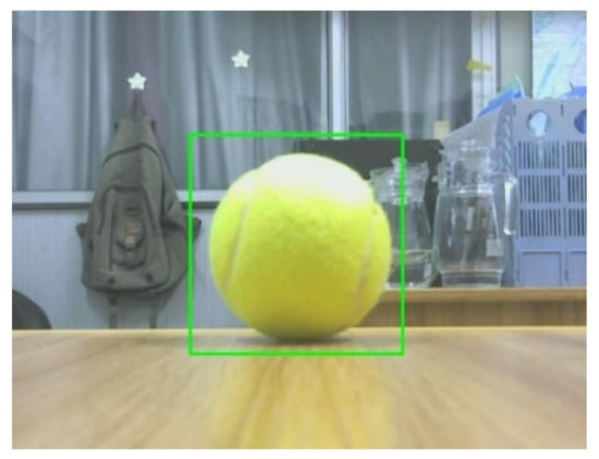
Figure 8.
Cascade classifier-based recognition of tennis balls.
The use of cascade classifier has a higher recognition rate than only using color and contour features to identify tennis balls and will not easily regard objects with similar color or contour as tennis balls; however, there are strict requirements on recognition distance and ambient light, and factors such as far distance, strong or weak light, and the proximity of other objects with similar color or contour can easily lead to poor recognition effect of cascade classifier. Therefore, it is also necessary to consider the design of a scheme that is less affected by the environment, i.e., stronger anti-interference ability, and on this basis the recognition distance of the robot can be farther to ensure that the robot can obtain the location information of the tennis ball smoothly and efficiently in the actual tennis ball picking operation.
3.3. The Recognition Algorithm of Tennis Ball Based on Deep Learning
In the practical application of deep learning method, the characteristics of samples, the size of sample batches, the setting of hyperparameters, data pre-processing, gradient estimation, etc., are all important factors that need to be studied and analyzed. Some factors’ proper training zones even cannot be determined until they are tested many times by deep learning [19].
We built an Anaconda virtual environment on a computer workbench before training the features of tennis samples, and then built Tensorflow deep learning framework on the basis of this virtual environment. Tensorflow is a symbolic mathematical system based on data programming, which is widely used for programming various machine learning algorithms, and its predecessor is Google’s neural network algorithm library DistBelief.
The experimental workflow is as follows:
- Acquiring samples is a very important step before carrying out deep learning work. Suitable samples can better reflect the main features of the object to be recognized and help in the establishment of the training model. Before training the model, the author collected a total of more than 1000 samples of original tennis images with different lighting conditions, different background information, and different distances, respectively. In order to increase the number of image samples for training, the data expansion operation (horizontal mirror flip and vertical mirror flip) is performed on these 1000 tennis images so that the number of tennis image samples exceeds 3000, taking into account the different states of the tennis ball in the actual situation as much as possible to ensure that the robot can have a better recognition rate of the tennis ball in the actual work of picking up the tennis ball.
Some of the tennis ball image samples collected by the author are shown in Figure 9. Considering the characteristics of deep learning, only one tennis ball is included in each image, which is to highlight the main features of the tennis ball and to avoid the computer recognizing several tennis balls as a whole, which is beneficial for the robot to distinguish multiple tennis balls in the ingested image recognition [20].
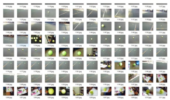
Figure 9.
Sample tennis ball images.
- 2.
- After acquiring the image samples, the samples need to be pre-processed to express the target to be recognized with the subject features of the target in the form of data. The generated expression data are recorded on the corresponding files, which are used in deep learning to train a training model dedicated to the recognition of tennis balls, because the distribution range of the feature taking values of each dimensional feature of the sample often varies widely due to the different sources and units of measure, and when calculating the Euclidean distance between different samples the features taking larger values play a dominant role [21]. Therefore, the deep learning method based on similarity comparison requires data pre-processing of the samples to normalize the features of each dimension to the same interval, which eliminates the correlation between individual features and thus obtains a better training result. However, the object to be recognized in this paper is only a tennis ball, which is round in the image, and the color and pattern of each tennis ball are not obviously different from each other, so the data pre-processing of the tennis ball sample needs to make the outline of the tennis ball distinguish from the background, and the color of the tennis ball also needs to be distinguished from other objects through special processing, combining the two aspects of appeal to peel the tennis ball from the image background so as to facilitate the subsequent model training.
In this paper, we use the labeling tool, labelme, to label the tennis balls in the collected sample images by carefully depicting the outline of the tennis balls in the images to distinguish them from the background of the images, save the labeling results to generate json type files, and transform these json type files to generate the description files for training. The saved json file and the converted description file are shown in Figure 10.

Figure 10.
Json files and the description files.
However, the above annotation method is manual annotation, and the image samples collected by the author are large, and it takes a lot of time to annotate all images manually, and the accuracy of subsequent annotation may be significantly reduced because there are too many image samples to be annotated and human energy is limited. Therefore, to reduce the workload of the experimenter and to improve the quality of the annotated images at the same time, the theory of the detection Hoff circle algorithm in OpenCV is introduced.
The equation of the circle in the Cartesian coordinate system is:
As shown in Figure 11, a particular circle in the Cartesian coordinate system is uniquely determined by three parameters (x-coordinate, y-coordinate, and radius r of the circle). To detect a circle, the circle is transformed from the Cartesian coordinate system to the Hough space, i.e., a circle in the Cartesian coordinate system is transformed into a point in the Hough space, and a point of a circle in the Cartesian coordinate system is transformed into a cone in the Hough space. When using the Hough circle detection theory, the Canny edge detection is first performed on the original image to obtain the binary map, and then the Sobel operator is executed so that the domain gradient values of all pixels are calculated, and finally the circle center and radius of the circle in the image are estimated [22].
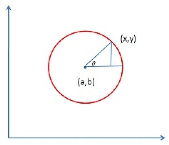
Figure 11.
Circles in the Cartesian coordinate system.
Therefore, the image sample pre-processing steps are as follows:
- First, some highly defined and distinctive tennis image samples are labeled using labelme as shown in Figure 12, and the description files generated from these samples are subjected to deep learning to generate a simple training model with a large number of parameters;
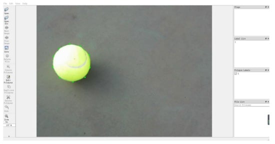 Figure 12. Sample of marked tennis images.
 - Then use these models to generate masks, and then use OpenCV’s detection Hough circle image theory to find the boundaries of the masks, and write these aliased nodes found to json files;
- Finally, use labelme to read in these json files and correct their boundary data.
This significantly reduces the workload of human calibration of the tennis image samples.
At the same time, since the tennis ball has a circular outline with clear and simple features, the corrected boundary data fit more closely to the pixel boundary values of the tennis ball in the image sample, making the accuracy of annotation higher compared with that of manual annotation.
- 3.
- Once the pre-processing of tennis image samples is completed and checked, the description file generated by the above annotation can be trained and learned using the corresponding deep learning algorithm to generate a training model specifically for tennis ball recognition. In this paper, we set up the Anaconda virtual environment on the computer workbench before training the tennis ball image samples, and then build the Tensorflow deep learning framework on the basis of this virtual environment. Tensorflow is a symbolic mathematical system based on data programming and is widely used in the programming of various machine learning algorithms.
As shown in Figure 13, Mask R-CNN is a simple, flexible, versatile, and fast instance segmentation framework, which is based on the Faster R-CNN framework of convolutional neural networks. The mask branch is a small full convolutional network on Region of Interest ((RoI) which means “box on feature map”), parallel to the classification and border regression branches that generates high quality segmentation masks on a pixel-by-pixel predictive basis on each RoI, but the increase in computational effort is not significant [23]. Referring to Figure 2, the Faster R-CNN is a fully connected layer of the convolutional neural network based on Figure 2 followed by a classification branch and a regression branch, while the Mask R-CNN is a mask branch added to the Faster R-CNN in parallel with the classification branch and the regression branch.
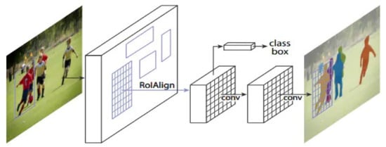
Figure 13.
The Mask R-CNN framework.
As shown in Figure 14, the black part is the original Faster R-CNN network structure, and the red part is the modified mask part based on the Faster R-CNN network, thus forming the Mask R-CNN network.
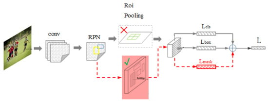
Figure 14.
Adding mask branches based on Faster R-CNN framework.
Before training the image samples, we also need to pay attention to the loss function of the training model. The loss function is used to estimate the degree of inconsistency between the predicted and true values of the model, and the smaller the loss function, the better the robustness of the model. As the loss function is mainly used in the training phase of the model, after each batch of training data are input to the model, the predicted value is output through forward propagation, and then the difference between the predicted value and the true value is calculated through the loss function, which is the loss value; after the loss value is obtained, the model updates each parameter through backward propagation to reduce the gap between the true value and the predicted value so that the predicted value generated by the model is closer to the true value. The model is then back-propagated to update each parameter to reduce the difference between the true value and the predicted value, so that the predicted value generated by the model is closer to the true value, thus achieving the purpose of learning [24].
The literature [25], a paper published by Kaiming He et al. to improve the generated Mask R-CNN based on Faster R-CNN, explains in detail the process of generating Mask R-CNN based on Faster R-CNN and summarizes the loss functions of Faster R-CNN and Mask R-CNN. Therefore, in order to reasonably combine different loss functions, bring into play the advantages of each loss function, and construct a distance-based or probability distribution-based measure of feature space that best expresses the main features of the data, the Mask-RCNN chosen to be used in this paper as a multi-task instance segmentation network model is to add a branching network to the Faster-RCNN, i.e., to the Faster RCNN model is covered with a mask to segment the target pixels while achieving target detection. Therefore, the loss function of the model is calculated by adding the mask loss to the bbox regression loss and the class loss.
As shown in Formula (2), the first two terms (, ) of the combined Mask R-CNN loss function are the same as those of the Faster R-CNN loss function. the loss of Faster R-CNN is mainly divided into the loss of RPN and the loss of Fast R-CNN, and both RPN loss and Fast R-CNN loss include classification loss and regression loss. Their specific loss function formulas are shown in Formula (3):
Let us first discuss the classification loss function . As shown in Formula (4), where the RPN network generates anchors that are divided into foreground and background only, with the label of foreground being 1 and the label of background being 0. In the process of training RPN, 256 anchors are selected, and that is 256. The loss here is the classical binary cross-entropy loss, is the anchor predicted as the target. The probability of the GT label is:
is 1 in the presence of objects (positive) and 0 in the absence of objects (negative), meaning that only the foreground is computed as loss and the background is not computed as loss. Moreover, (,) is the logarithmic loss for both categories (target and non-target).
The classification loss of RPN is the cross-entropy loss of binary classification, while Fast R-CNN is the cross-entropy loss of multi-classification. A total of 128 RoIs are selected in Fast R-CNN during training, i.e., = 128, and the values of labels are 0 to 4.
Regarding the regression loss function , as shown in Formula (7), where = {,,,} is a vector representing the offset predicted by the anchor, RPN training phase (RoIs, Fast R-CNN training phase), and x, y, w, and h represent the center coordinates, width, and height of the anchor box anchor, respectively. is the same dimension as vector that represents the actual offset of anchor, RPN training phase (RoIs, Fast R-CNN training phase) with respect to GT:
R in Formula (8) is the function, with the difference that here = 3, RPN training phase (= 1, Fast R-CNN training phase):
Among them,
For each anchor, is multiplied after calculating the part. As mentioned before, is 1 in the presence of objects (positive) and 0 in the absence of objects (negative), implying that only the foreground is calculated as loss and the background is not. The parameter can be interpreted as a weight parameter introduced to balance the classification loss and the regression loss.
Finally, the mask loss function is discussed. For each RoI, the mask branch has an output of K × m × m dimensions, which encodes K masks of size m × m, and each RoI has K categories. We use the per-pixel sigmoid and define it as the average binary cross-entropy loss. An RoI corresponding to the kth category in GT is defined only over the kth mask (the other k-1 masks output no contribution to the overall loss). Our definition allows the network to generate a mask for each class without competing with other classes; we rely on the class labels predicted by the classification branch to select the output mask. This differs from semantic segmentation using FCN, which typically uses a per-pixel sigmoid and a multinomial cross-entropy loss, in which case there is competition between masks; since we use a per-pixel sigmoid and a binary loss, there is no competition between the different masks. Experience shows that this can improve the effectiveness of instance segmentation. The specific formula for the loss function of the mask is shown in Formula (11):
where means 1 when the kth channel corresponding to the target is the real category, otherwise 0; y means the label value of the mask at the current position, 0 or 1; x means the output value at the current position, and sigmoid(x) means the result of the output x transformed by the sigmoid function.
After the loss function is combined, the best optimization method is found by the special layer of target detection (RoIAlign), the number of GPU cores, the total number of iterations of the model, the number of rounds in each iteration (one round for updating the training set samples), the number of training steps in each round, the number of check steps in each round, the fine-tuning parameters of the rounds, etc. RoIAlign is a regional feature aggregation method to solve the problem of region mismatch caused by twice quantization in the RoI pooling operation in neural networks, and to improve the model accuracy by generating a fixed range of features [26]. The rest of the iterative layers and rounds are used to tune the structure of the model and improve the learning efficiency and stability of the model [27].
4. Experimental Results and Analysis
All the tests in this work are carried out on the same hardware and software platform. The environmental parameters are listed in Table 1.

Table 1.
Hardware and software parameters.
As shown in Figure 15, the internal process of training tennis image samples based on Mask R-CNN convolutional network model is as follows:
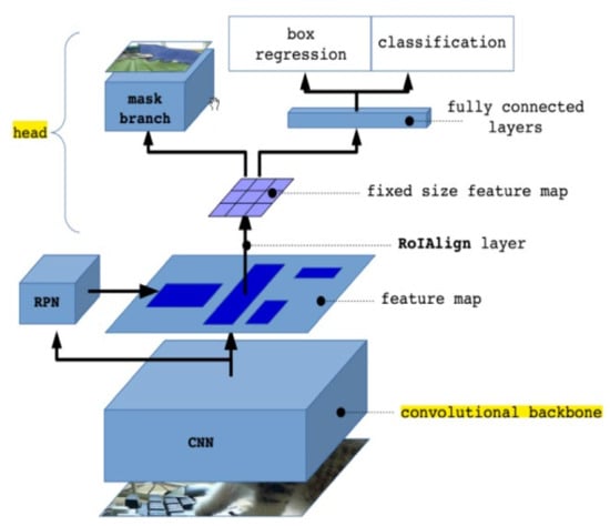
Figure 15.
Training flowchart.
- Input the pre-processed image samples into the pre-trained neural network so as to obtain the corresponding feature map;
- Predetermine an RoI for each point in this feature map so as to obtain multiple candidate RoIs;
- Feed these candidate RoIs into the RPN network for binary classification (foreground or background) and BB regression to filter out some of the candidate RoIs;
- Perform RoIAlign operations on these remaining RoIs (i.e., first corresponding the coordinates of the original image and the feature map, and then corresponding the features of the feature map to the original image);
- Transfer the RoI of these RoIAlign operations into the mask region (mask branch in Figure 15) and the fully connected layer region of the convolutional network, respectively;
- Use the RoIs transmitted into the fully connected layer in the fully connected layer to map the feature space computed by the convolutional and pooling layers into the sample tag space, thus enabling these RoIs to perform regression and classification operations (box regression and classification in Figure 15). In this case, perform FCN operations inside each RoI.
The loss function data of the training models at different iteration levels were recorded by setting the number of ROIs per sample in Mask R-CNN convolutional network and Faster R-CNN convolutional network to 100, the number of GPU cores to 2, 100 rounds of iterations per layer, 100 training steps per round, 50 calibration steps per round, and 10 fine-tuning parameters per round. Since Mask R-CNN is formed based on Faster R-CNN with the addition of mask branches which are parallel to the classification and regression branches, their classification loss functions and regression loss functions are the same, so the classification loss functions and regression loss functions of the models trained based on these two neural networks can be compared separately. In order to show the comparison results more intuitively, the more representative loss function iteration charts are selected in Figure 16, Figure 17, Figure 18, Figure 19, Figure 20 and Figure 21:
(1) The total number of iterations of the model is 10:

Figure 16.
Mask R-CNN loss function 1. (a) Class loss (b) bbox loss.

Figure 17.
Faster R-CNN loss function 1. (a) Class loss, (b) bbox loss.
(2) The total number of iterations of the model is 20:

Figure 18.
Mask R-CNN loss function 2. (a) Class loss, (b) bbox loss.

Figure 19.
Faster R-CNN loss function 2. (a) Class loss, (b) bbox loss.
(3) The total number of iterations of the model is 30:

Figure 20.
Mask R-CNN loss function 3. (a) Class loss, (b) bbox loss.

Figure 21.
Faster R-CNN loss function 3. (a) Class loss, (b) bbox loss.
Figure 16, Figure 17, Figure 18, Figure 19, Figure 20 and Figure 21 show the iterative plots of classification loss function and regression loss function of Mask R-CNN and Faster R-CNN under different iteration levels of the models, respectively. Among them, the blurrier curves in Figure 16, Figure 17, Figure 18, Figure 19, Figure 20 and Figure 21 are the actual decreasing curves of the loss function, and the brighter lines are the smoothed curves after setting the smoothing factor to 0.6, which makes the decreasing process of the loss function more intuitive. Moreover, the grids in some of these charts are denser, which is because some of the loss functions drop to very small, and the generated charts are somewhat adjusted and compressed in order to represent these points clearly.
Since Mask R-CNN has more mask branches than Faster R-CNN, Mask R-CNN also needs to calculate the loss function value of the mask. The loss function curves of Mask are plotted in Figure 22, Figure 23 and Figure 24 (where Figure 22 is consistent with the parameter settings of Figure 16, Figure 23 is consistent with the parameter settings of Figure 18, and Figure 24 is consistent with the parameter settings of Figure 20):
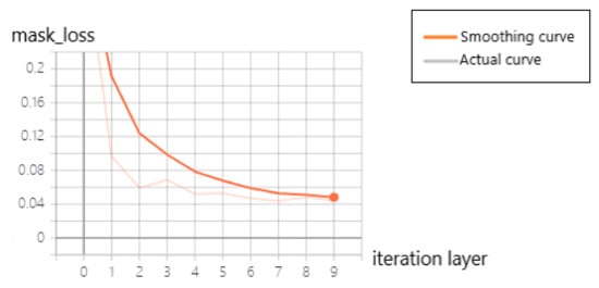
Figure 22.
Mask loss of Mask R-CNN 1.
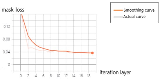
Figure 23.
Mask loss of Mask R-CNN 2.
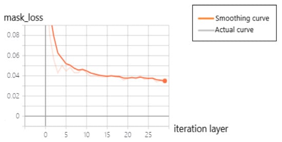
Figure 24.
Mask loss of Mask R-CNN 3.
The final values of various loss functions of Mask R-CNN at different iteration levels in the experiments are summarized in a table for comparison, as shown in Table 2:

Table 2.
Detailed loss function data of Mask R-CNN at different iteration levels.
The effectiveness of the improved and optimized Mask R-CNN convolutional network-based recognition tennis algorithm is summarized and compared with the traditional color-and-contour-based recognition tennis algorithm, cascade classifier-based recognition tennis, and Faster R-CNN convolutional network-based recognition tennis algorithm for practical detection, which can be obtained in Table 3:

Table 3.
Comparison of tennis ball recognition results using different recognition algorithms.
As shown in Table 3, the Mask R-CNN-based convolutional network improved and optimized recognition tennis algorithm has higher recognition accuracy and longer recognition distance for tennis balls than other recognition tennis algorithms. However, the recognition speed of the Mask R-CNN-based recognition algorithm is lower than that of the Faster R-CNN-based recognition algorithm, because the Mask R-CNN-based recognition algorithm also must predict the value of the mask, i.e., the optimization algorithm used in this paper sacrifices a little detection speed, but effectively improves the recognition effect of the tennis ball and enhances the robustness of the recognition algorithm to the external environment.
Figure 25 shows the recognition of tennis balls indoors and outdoors with the improved and optimized algorithm based on Mask R-CNN convolutional network. In this case, the mask outline of the tennis ball is depicted with a solid line in (b) in Figure 25, while the image of the recognized tennis ball is marked with a dashed box in order to distinguish it from the solid line.
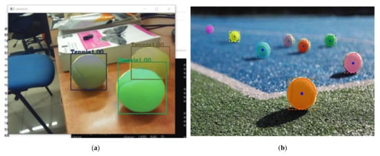
Figure 25.
Recognition effect diagram. (a) Identifying tennis balls indoors, (b) identifying tennis balls outdoors.
As can be seen from Figure 16, Figure 17, Figure 18, Figure 19, Figure 20 and Figure 21, the classification loss function and regression loss function of Mask R-CNN and Faster R-CNN neural networks significantly decrease in the interval between iteration layers 0 and 5. As the feature parameters on the training set samples are adjusted to delineate the main image features of the tennis ball, the model gets initial convergence, at this time, if the model is to be further trained, the gradient descent-based optimization method needs to reduce the learning rate of the model so that the learning rate is not too high resulting in the loss function values not converging; however, the learning rate cannot be reduced too much, otherwise the model will converge very slowly. Therefore, from Figure 16, Figure 17, Figure 18, Figure 19, Figure 20 and Figure 21, we can see that the curves of the classification loss function and regression loss function of the two neural networks tend to fall flat, and the learning rate of the training model has a more obvious reduction: one is to ensure that the loss function fluctuates less and always decreases, and the other is to ensure the stable convergence of the training model. After the number of iterations of the training model exceeds 20, the learning rate further decreases and the model with recorded image features converged to a more complete degree, although there is room for learning and training, the convergence of the model is not obvious at this time and can be observed only by using electronic devices; after the number of iterations of the model reaches 30, the decline of the loss function curve is minimal and tends to be stable, which means that the model generated by the tennis sample at this time converged to a more appropriate level. The model converged to a more suitable degree.
Finally, the relevant loss function values are recorded in Table 2. Observing Table 2, it is found that the classification loss function values and regression loss function values of Mask R-CNN match the curves in Figure 16, Figure 17, Figure 18, Figure 19, Figure 20 and Figure 21. The total loss function (loss) keeps decreasing as the number of iterative layers increases. The classification loss function (class loss) is combined with the regression loss function (bbox loss) and the mask loss function (mask loss) to ensure stable convergence of the model, so there are ups and downs, but the fluctuations are not large and the trend of decrease is maintained. The decline of the regression loss function (bbox loss), classification loss function (class loss), and mask loss function (mask loss) together constitute the convergence of the training model.
5. Conclusions
Considering the complexity and the effectiveness of the use of different recognition algorithms, as well as the main working environment of the robot, we provide two methods of tennis ball recognition: the color-and-contour-based method and the cascade classifier-based method. Firstly, the traditional method of searching for tennis balls based on color and contour is vulnerable to the environment and obstacles, while the other method has a very small identification distance and is more demanding on the working environment. Above all, in order to improve the efficiency and anti-interference ability of the robot in recognizing tennis balls, deep learning-based recognition of tennis balls is chosen as the method of this paper.
In this paper, we first pre-processed the collected tennis ball samples, and used deep learning methods to learn and train the samples to optimize the robot’s recognition algorithm for tennis balls. Based on the loss function theory of Mask-RCNN, we compare the iterative charts of classification loss function and regression loss function of Mask R-CNN and Faster R-CNN under the same parameters. Then we conclude that when the number of RoIs per sample in the neural network is set to 100, the number of GPU cores is 2, the neural network iterates 100 rounds per layer, the number of training steps per round is 100, the number of checking steps per round is 50, the fine-tuning parameters per round is 10, and the total number of model iterations is 30, Mask R-CNN has a better training effect on the collected tennis ball samples than Faster R-CNN, and the recognition rate of the model based on Mask R-CNN is 92% for tennis balls.
By examining the model generated by the above parameter settings, the following conclusions can be drawn: First, the experimental design of an optimized algorithm suitable for tennis ball sample collection will greatly improve the efficiency of the tennis ball pickup robot and enable real-time detection. Second, by applying the sample and training model optimization algorithms described in this paper, the recognition of tennis balls by the tennis ball pickup robot can reduce the influence of environmental factors. Finally, because the tennis ball sample data were iterated through 30 layers of neural networks, the generated model is stable and easy to call, reducing the user’s time.
Author Contributions
Conceptualization, D.W. and A.X.; methodology, A.X.; software, D.W.; validation, D.W. and A.X.; investigation, D.W.; writing—original draft preparation, D.W.; writing—review and editing, D.W. and A.X.; visualization, D.W.; supervision, A.X.; project administration, A.X.; data curation D.W. All authors have read and agreed to the published version of the manuscript.
Funding
This research received no external funding.
Institutional Review Board Statement
Not applicable.
Informed Consent Statement
The authors declare that the studies described in this paper do not involve humans.
Data Availability Statement
The data presented in this study are available in this paper.
Conflicts of Interest
The authors declare that they have no known competing financial interests or personal relationships that could have appeared to influence the work reported in this paper.
Code or Data Availability
Authors can confirm that all relevant data are include in the article.
Ethics Approval
The experiment passed ethical approval.
Consent to Participate
Consent to the participation of experimentalists.
Consent for Publication
This paper is approved for publication.
References
- Burnar, V.T. The new ‘youth fountain’ of Romania: How tennis overtook gymnastics as the premier juvenile sport of the country. J. Pract. Comunitare Pozitive 2020, 20, 47–68. [Google Scholar] [CrossRef]
- Hong, F.; He, G. The Asian games, Asian sport and Asian politics. In The Routledge Handbook of Sport in Asia; Routledge: Evanston, IL, USA, 2020; pp. 493–504. [Google Scholar]
- Zhou, H.; Zhou, S.; Yu, J.; Zhang, Z.; Liu, Z. Trajectory optimization of pickup manipulator in obstacle environment based on improved artificial potential field method. Appl. Sci. 2020, 10, 935. [Google Scholar] [CrossRef]
- Peng, Y.; Zhang, T.; Fu, Q. Research on real-time evaluation algorithm of human movement in tennis training robot. Microprocessors Microsyst. 2021, 81, 103683. [Google Scholar] [CrossRef]
- Chen, Y.; Wang, S. Poultry carcass visceral contour recognition method using image processing. J. Appl. Poult. Res. 2018, 27, 316–324. [Google Scholar] [CrossRef]
- Paisitkriangkrai, S.; Shen, C.H.; van den Hengel, A. Asymmetric Pruning for Learning Cascade Detectors. IEEE Trans. Multimed. 2014, 16, 1254–1267. [Google Scholar] [CrossRef]
- Ortiz-Jiménez, G.; Modas, A.; Moosavi-Dezfooli, S.M.; Frossard, P. Optimism in the Face of Adversity: Understanding and Improving Deep Learning through Adversarial Robustness. Proc. IEEE 2021, 109, 635–659. [Google Scholar] [CrossRef]
- Safkhani, M.; Rostampour, S.; Bendavid, Y.; Bagheri, N. IoT in medical & pharmaceutical: Designing lightweight RFID security protocols for ensuring supply chain integrity. Comput. Netw. 2020, 181, 107558. [Google Scholar]
- Shivappriya, S.N.; Priyadarsini, M.J.P.; Stateczny, A.; Puttamadappa, C.; Parameshachari, B.D. Cascade Object Detection and Remote Sensing Object Detection Method Based on Trainable Activation Function. Remote Sens. 2021, 13, 200. [Google Scholar] [CrossRef]
- Zhou, C.; Li, F.; Cao, W.; Wang, C.; Wu, Y. Design and implementation of a novel obstacle avoidance scheme based on combination of CNN-based deep learning method and liDAR-based image processing approach. J. Intell. Fuzzy Syst. 2018, 35, 1695–1705. [Google Scholar] [CrossRef]
- Gu, S.; Zeng, W.; Jia, Y.; Yan, Z. Intelligent Tennis Robot Based on a Deep Neural Network. Appl. Sci. 2019, 9, 3746. [Google Scholar] [CrossRef]
- Wu, Y.C.; Feng, J.W. Median-Pi artificial neural network for forecasting. Neural Comput. Appl. 2019, 31, 307–316. [Google Scholar]
- Wu, Y.C.; Feng, J.W. Development and Application of Artificial Neural Network. Wirel. Pers. Commun. 2018, 102, 1645–1656. [Google Scholar] [CrossRef]
- Tian, Y.H. Artificial Intelligence Image Recognition Method Based on Convolutional Neural Network Algorithm. IEEE Access 2020, 8, 125731–125744. [Google Scholar] [CrossRef]
- Zhou, D.X. Deep distributed convolutional neural networks: Universality. Anal. Appl. 2018, 16, 895–919. [Google Scholar] [CrossRef]
- Romani, S.; Sobrevilla, P.; Montseny, E. Variability estimation of hue and saturation components in the HSV space. Color Res. Appl. 2012, 37, 7539. [Google Scholar] [CrossRef]
- Torii, A.; Imiya, A. The randomized-Hough-transform-based method for great-circle detection on sphere. Pattern Recognit. Lett. 2007, 28, 1186–1192. [Google Scholar] [CrossRef]
- Tian, H.; Duan, Z.; Abraham, A.; Liu, H. A novel multiplex cascade classifier for pedestrian detection. Pattern Recognit. Lett. 2013, 34, 1687–1693. [Google Scholar] [CrossRef]
- Kim, K.; Young, J. Secure Object Detection Based on Deep Learning. J. Inf. Process. Syst. 2021, 17, 571–585. [Google Scholar]
- Lim, S.M.; Oh, H.C.; Kim, J.; Lee, J.; Park, J. LSTM-Guided Coaching Assistant for Table Tennis Practice. Sensors 2019, 18, 4112. [Google Scholar] [CrossRef]
- Liang, H.; Sun, X.; Sun, Y.; Gao, Y. Text feature extraction based on deep learning: A review. EURASIP J. Wirel. Commun. Netw. 2017, 1, 211. [Google Scholar] [CrossRef]
- Yang, G.; Hu, J.P.; Hou, Z.C.; Zhang, G.; Wang, W.J. A new hough transform operated in a bounded cartesian coordinate parameter space. IET Image Process. 2022, 16, 2282–2295. [Google Scholar] [CrossRef]
- Zhang, Q.H.; Chang, X.N.; Bian, S.F.B. Vehicle-Damage-Detection Segmentation Algorithm Based on Improved Mask RCNN. IEEE Access 2020, 8, 6997–7004. [Google Scholar] [CrossRef]
- Rengasamy, D.; Jafari, M.; Rothwell, B.; Chen, X.; Fgueredo, G.P. Deep Learning with Dynamically Weighted Loss Function for Sensor-Based Prognostics and Health Management. Sensors 2020, 20, 723. [Google Scholar] [CrossRef] [PubMed]
- He, K.; Gkioxari, G.; Dollar, P.; Girshick, R. Mask R-CNN. IEEE Trans. Pattern Anal. Mach. Intell. 2017, 42, 386–397. [Google Scholar] [CrossRef] [PubMed]
- Kim, S.Y.; Lee, E.K.; Ho, Y.S. Generation of ROI Enhanced Depth Maps Using Stereoscopic Cameras and a Depth Camera. IEEE Trans. Broadcast. 2008, 54, 732–740. [Google Scholar] [CrossRef]
- Yu, J.B.; Yan, X.F. A new deep model based on the stacked autoencoder with intensified iterative learning style for industrial fault detection. Process Saf. Environ. Prot. 2021, 153, 47–59. [Google Scholar] [CrossRef]
Publisher’s Note: MDPI stays neutral with regard to jurisdictional claims in published maps and institutional affiliations. |
© 2022 by the authors. Licensee MDPI, Basel, Switzerland. This article is an open access article distributed under the terms and conditions of the Creative Commons Attribution (CC BY) license (https://creativecommons.org/licenses/by/4.0/).