Abstract
In this paper, we present a monitoring program of loss control prevention for airlines to enhance aviation safety and operational efficiency. The assessments of dynamic stability characteristics based on the approaches of oscillatory motion and eigenvalue motion modes for jet transport aircraft response to sudden plunging motions are demonstrated. A twin-jet transport aircraft encountering severe clear-air turbulence in transonic flight during the descending phase was examined as the study case. The flight results in sudden plunging motions with abrupt changes in attitude and gravitational acceleration (i.e., the normal load factor) are provided. Development of the required thrust and aerodynamic models with the flight data mining and the fuzzy logic modeling techniques was carried out. The oscillatory derivatives extracted from these aerodynamic models were then used in the study of variations in stability characteristics during the sudden plunging motion. The fuzzy logic aerodynamic models were utilized to estimate the nonlinear unsteady aerodynamics while performing numerical integration of flight dynamic equations. The eigenvalues of all motion modes were obtained during time integration. The positive real part of the eigenvalues is to indicate unstable motion. The dynamic stability characteristics during sudden plunging motion are easily judged by the values in positive or negative. The present quantitative assessment method is an innovation to examine possible mitigation concepts of accident prevention and promote the understanding of aerodynamic responses of the jet transport aircraft.
1. Introduction
Aircraft performance data for aircraft autopilots and some training-level flight simulators design are generally obtained from flight testing under normal flight conditions. It is impossible to take all flight conditions into account in the design process of transport aircraft. Some flight conditions, e.g., in-flight abrupt descent in clear-air turbulence (CAT), are not easy to test in airworthiness certification, which may lead to the aircraft loss of control in commercial service operation. The flight mechanism of off-nominal conditions cannot easily be simulated by wind tunnel tests, and it is not possible to directly perform flight tests with real aircraft. In other words, the design value of aerodynamic performance is inconsistent with the actual aerodynamic performance during the flight operations. It is appropriate that off-nominal flight conditions cannot be combined with aircraft design and flight simulators [1]. More importantly, the pilots cannot gain much experience in these flight conditions.
The adverse weather related to off-nominal flight conditions includes (but is not limited to) heavy rain, convective storms [2], turbulence [3,4], crosswind [5,6], wind shear [7,8], and in-flight icing [9,10]. Adverse weather impacts the flight safety of transport aircraft and the operational efficiency of air traffic management. An innovative commercial flight route planning tool is developed to avoid the deep convective storms [2]. This program provides an overview to establish a better air route based on original trajectory operations for safe, efficient, and comfortable operating flights to the airlines.
Among the different adverse weathers, clear-air turbulence is important in flight safety since it is hard to detect and predict. Clear-air turbulence is the leading cause of serious personal injuries in non-fatal accidents of commercial aircraft [11]. One main type of motion that causes flight injuries in clear-air turbulence is the sudden plunging motion with abrupt changes in attitude and gravitational acceleration (i.e., the normal load factor) [12]. The assessment of flying qualities during sudden plunging motion was presented for an aged twin-jet transport aircraft encountering severe clear-air turbulence through digital six degree-of-freedom (6-DOF) flight simulations. The important process of the method is to numerically integrate the 6-DOF equations of motion and simultaneously determine the eigenmodes of motion at every instant. The longitudinal equations are coupled with the lateral-directional equations, and some nonlinear effects are incorporated, which is an advantage of 6-DOF flight simulation [13]. Unfortunately, with that approach, it was difficult to identify the individual modes of motion from these eigenvalues from one instant to another because of the rapid changes in aerodynamic forces and moments in turbulence.
In Ref. [11], an aged twin-jet transport aircraft was tested. The static aeroelastic effect was significant when the transport aircraft sustained instantaneous high g-loads in severe clear-air turbulence. Any structural deformation with static aeroelastic effects caused by flight loads would change certain aerodynamic parameter values. However, that article did not provide the corresponding relationship between the static aeroelastic effect and eigenvalue motion modes.
This article presents flight data mining and the fuzzy logic modeling of an artificial intelligence technique to establish nonlinear and unsteady aerodynamic models for six aerodynamic coefficients based on the flight data of a new twin-jet transport aircraft with the service year of only 11 months. The new aircraft has fewer static aeroelastic effects in comparison with the aged one, and even those of the new one can be negligible [14]. This new twin-jet encountered severe clear-air turbulence twice during the descending phase. The oscillatory derivatives extracted from the aerodynamic models were used to study the dynamic stability characteristics during the sudden plunging motion. The longitudinal and lateral-directional motion modes were analyzed through digital flight simulation based on decoupled dynamic equations of motion. The eigenvalue equations were formulated in the form of polynomials and solved. The eigenvalues for short-period, phugoid (long-period), Dutch roll, spiral, and roll modes of motion were estimated based on the damping ratio and undamped natural frequency. A positive real part of the eigenvalues is to indicate unstable motion. The dynamic stability characteristics during sudden plunging motion are easily judged by the values in positive or negative. The present approach is an innovation to examine possible mitigation concepts of accident prevention for airlines to enhance aviation safety and operational efficiency.
2. Methodology
2.1. Flight Data Mining Technology
The input data for fuzzy logic modeling were extracted from post-flight data. There are many flight parameters recorded by FDRs (Flight Data Recorders) or QARs (Quick Access Recorders), but some of them are not related to the current study, such as light signs, landing gear retracting, etc. The steps are to collect and organize a large amount of data and obtain the required information for specific analysis and applications; this process is called flight data mining [15]. The flight data mining process is divided into two parts: the development of a nonlinear and unsteady aerodynamic database and the aerodynamic models.
2.2. Development of Nonlinear and Unsteady Aerodynamic Database
This section describes the development process of the demand data selection, data frequency upscaling and data make-up, compatibility check, and input information of aircraft main geometry and moment of inertia data. The flowchart of each step is shown in Figure 1.
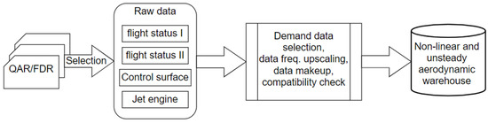
Figure 1.
Flowchart for the development of a nonlinear and unsteady aerodynamic data database.
Before developing a nonlinear and unsteady aerodynamic database, one must ensure that the selected parameters and corresponding data are those required for the study. The parameters and corresponding data required for the current study include the following items:
- (1)
- To select the required flight status, flight control surface, and engine raw data for a specific flight number from the actual flight QAR or FDR data.
- (2)
- The main geometric and moment of inertia data include appearance size, wingspan, average chord length, wing area, etc. Most are public data of aircraft manufacturers and can be obtained via the Internet. However, the thrust performance of the entire aircraft is non-public data and must be obtained from the Flight Planning and Performance Manual (Boeing Series) or Flight Crew Operation Manual (Airbus Series).
The frequency of each parameter sensor is different, from 1 Hz to 8 Hz, due to the properties and characteristics of the parameters [16]. For example, attitude angles such as roll, pitch, and heading angles are 4 Hz; aileron and elevator angles are 2 Hz; the vertical acceleration sampling rate is 8 Hz. To preserve the properties and characteristics of each parameter, it is necessary to avoid high-frequency data loss, so the frequency of all original data sampling is uniformly arranged to 8 Hz.
The data frequency increase and make-up of this research are developed based on the method of monotone cubic spline interpolation [17]. This method is commonly used in aircraft flight test analysis to provide a smooth curve. Data upscaling and data completion of blanks are important steps for the aerodynamic database to have high accuracy and reliability in applications for operational efficiency enhancement of transport aircraft.
2.3. Compatibility Check
Typically, the longitudinal, lateral, and vertical accelerations (ax, ay, az) along the (x, y, z)-body axes of aircraft, as well as the angle of attack α, Euler angles (ϕ, θ, and ψ), aileron deflection (δa), elevator (δe), rudder (δr), stabilizer (δs), etc., are available and recorded in the QAR or FDR of all transport aircraft. Since the recorded flight data may contain errors (or biases), compatibility checks are performed to remove them by satisfying the following kinematic equations [12,18]:
where g is the gravitational acceleration and V is the flight speed. Let the errors be denoted as , for ax, ay, az, etc., respectively. These errors are estimated by minimizing the squared sum of the differences between the two sides of Equations (1)–(6).
These equations in vector form can be written as:
where
where superscript “¯” stands for the mean value and the subscript “m” indicates the measured or recorded values. The cost function is defined as:
where Q is a weighting diagonal matrix with elements being 1.0 and is calculated with a central difference scheme with , which is the measured value of . The steepest descent optimization method is adopted to minimize the cost function. As a result of analysis, variables unavailable in the QAR or FDR, such as β, p, q, and r, are able to be estimated.
The above-mentioned unavailable variables in the QAR or FDR need initial values as a basis for correction, where the angular rates, such as p, q, and r, are obtained from derivatives of , , and with time by using the method of monotonic cubic interpolation. This interpolation method is used to connect the flight data in a continuous curve to obtain the slope of the curve. The value of β cannot be obtained from the derivative. The initial value of β is assumed to be 0 at the time of estimation, and it is calculated when Equation (6) is satisfied.
2.4. Aircraft Main Geometry and Moment of Inertia Data
The main objective of this article is to present a dynamic stability monitoring method based on the approach of oscillatory motion and eigenvalue motion modes for the twin-jet transport aircraft response to sudden plunging motions. The data of main geometry and moments of inertia are presented in Table 1.

Table 1.
Main geometry and moment of inertia data for the twin-jet transport aircraft.
2.5. Nonlinear and Unsteady Aerodynamic Database
The actual physical phenomenon of an aircraft flying in the atmosphere is the physical movement along the flight trajectory over time. Since all flight variables recorded are based on the body axes, it is more convenient to estimate the force and moment coefficients for aircraft on the same axis system as follows [19]:
(1) Force coefficients acting on the body axes of the aircraft:
(2) Moment coefficients about the body axes of the aircraft:
where m is the aircraft mass; is the dynamic pressure; S is the wing reference area; Cx, Cz, and Cm are the longitudinal aerodynamic force and moment coefficients; Cy, Cl, and Cn are the lateral-directional aerodynamic force and moment coefficients; and Ixx, Iyy, and Izz are the moments of inertia about the x-, y-, and z-axes, respectively. The products of inertia, Ixy, Ixz, and Iyz, are assumed to be zero in the present case but are included in the equations because non-zero values may be available in other applications. The terms Tx, Ty, Tz, and Tm represent the thrust contributions to the force in the direction of x-, y-, and z-axes and to the pitching moment, respectively.
The variables pq, qr, and pr in the Equations (15)–(17) are the product terms of two dependent variables, and the equations belong to the nonlinear differential equation system due to the existence of nonlinear terms. Nonlinear differential equations are difficult to solve mathematically, and the physical phenomena of motion are complicated [20]. In the physical sense, the product term of the two dependent variables is related, which is the coupling effect of nonlinear motion. The raw flight data of QAR or FDR can be used to establish a nonlinear and unsteady aerodynamic database through the steps of the flowchart in Figure 1.
The terms on the left-hand side of Equations (15)–(17) are rolling, pitching, and yawing moments. The moments due to inertia coupling on the right-hand side in Equations (15)–(17) will be produced due to the abrupt change in the flight attitude before and during the severe clear-air turbulence encounters.
2.6. Development of Nonlinear and Unsteady Aerodynamic Models
This section describes the development process of nonlinear and unsteady aerodynamic models, as shown in Figure 2. The flowchart of Figure 2 is based on the data of the nonlinear and unsteady aerodynamic database. The thrust data in aerodynamic database have been separated from aerodynamic coefficients. Model strucg-n, the numerical model structure, is set up through parameter selection, time segment selection, and sampling rate setting, and then goes through the refining process of fuzzy logic modeling to establish the required models. The operational efficiency enhancement can be studied after model defuzzification.
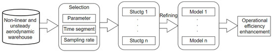
Figure 2.
Flowchart for the development of nonlinear and unsteady aerodynamic models.
,,, and are the axial thrusts along the body x-, y-, and z-coordinates and the pitching moment about the y-axis, respectively, in Equations (12)–(14) and (16). It is known from the various thrusts that the force and moment acting on the aircraft will be affected by the engines. Both thrust and aerodynamic forces are generated together, and the two effects cannot be accurately separated only from the flight record data during analysis. To accurately estimate the aerodynamic coefficient, it is necessary to obtain an accurate thrust value to separate the thrust effects; then, the accurate aerodynamic coefficients can be obtained [18].
Since the values of thrust for aircraft in flight cannot be directly measured in the current state of the art, they are not recorded by the QAR nor the FDR. The manufacturers of engines agreed that using parameters such as the Mach number, airspeed, flight altitude, temperature, rpm of the pressure compressors, and engine pressure ratios are adequate to estimate the engine thrust [21]. To study aircraft performance with fuel consumption, data from the flight manual for the fuel flow rate () at various altitudes (h), weights (W), Mach numbers (M), calibrated airspeed (CAS), and engine pressure ratios (EPRs) during cruise flight are utilized.
For the Pratt and Whitney turbofan engines, thrust (T) is defined by EPR, and the thrust model is set up as:
For GE or CFM turbofan engines, the rpm of the low-pressure compressor (N1) is used to set the level of thrust, so the thrust model is set up as:
In the present study, a twin-jet with GE turbofan engines under study is illustrated. The actual thrust in operation is obtained by using the recorded variables in the QAR, particularly the fuel flow rates. Once the thrust models are generated as a function with the flight conditions of climbing, cruise, and descending phases, we can estimate the thrust magnitude by inserting those flight data into the aerodynamic database.
When studying the nonlinear and unsteady aerodynamic characteristics of motion, it can be found that the nonlinear and unsteady aerodynamics with hysteresis [6,22,23] are affected by many parameters of motion state. The aerodynamic models developed by the fuzzy logic modeling method are suitable for aerodynamic research of coupling motion and can be used to enhance the operational efficiency of transport aircraft. The development process of nonlinear and unsteady aerodynamic models is shown in Figure 2.
Modeling means to establish the numerical relationship among certain variables of interest. In the fuzzy logic model, more complete necessary influencing flight variables can be included to capture all possible effects on aircraft response to structure deformations. The longitudinal main aerodynamics are assumed to depend on the following ten flight variables [22]:
The coefficients on the left-hand side of Equation (20) represent the coefficients of axial force (Cx), normal force (Cz), and pitching moment (Cm). The variables on the right hand side of Equation (20) denote the angle of attack (α), time rate of angle of attack (dα/dt, or ), pitch rate (q), longitudinal reduced frequency (k1), sideslip angle (β), control deflection angle of elevator (δe), Mach number (M), roll rate (p), stabilizer angle (δs), and dynamic pressure (). These variables are called the influencing variables. The roll rate is included here because it is known that an aircraft encountering hazardous weather tends to develop rolling, which may affect longitudinal stability. The variable of dynamic pressure is for estimation of the significance in structural deformation effects.
For the lateral-directional aerodynamics [22],
The coefficients on the left-hand side of Equation (21) represent the coefficients of side force (Cy), rolling moment (Cl), and yawing moment (Cn). The variables on the right-hand side of Equation (21) denote the angle of attack (α), sideslip angle (β), roll angle (ϕ), roll rate (p), yaw rate (r), lateral-directional reduced frequency (k2), control deflection angle of aileron (δa), control deflection angle of rudder (δr), Mach number (M), the time rate of angle of attack (), and the time rate of sideslip angle ().
Most representative of the numerical differentiation theory is the difference method. This paper uses the central difference method as follows.
Although the numerical differentiation method is used to obtain the derivative of a certain point of the function curve, it can also be applied to the derivative analysis of experimental data. However, the experimental data are scattered and discontinuous points, and interpolation must be used to connect the points into a continuous curve. Fuzzy logic modeling plays the function of interpolation. Fuzzy logic modeling is extremely important in the aerodynamic performance analysis of actual flight data. Two examples of applying the fuzzy logic modeling model to take derivatives are given.
The longitudinal stability derivative (Cmα) comes from the model of Cm. The aerodynamic derivative of the unsteady aerodynamic model can be calculated using the central interpolation method. The formula of the central difference method is as follows:
Cmα = [Cm (α + Δα, …) − Cm (α − Δα, …)]/2Δα
Δα = 0.1 degrees, which means that α changes up and down by 0.1 degrees, while all other variables remain unchanged.
The damping derivative (Clp) is proposed from the model Cl. The formula of the central interpolation method is as follows:
where Δp is in unit of deg/s.
Clp = [Cl (…, p + Δp, …) − Cl (…, p − Δ p, …)]/2Δp
The calculations of all other aerodynamic derivatives are derived from the same method in this paper.
2.7. Flight Simulation
Due to the rapid changes in aerodynamic forces and moments in turbulence, it is difficult to identify the individual modes of motion from these eigenvalues through digital 6-DOF flight simulations from one instant to another. Regarding the dynamic stability monitoring, one approach to solve this problem is to use the approximate modes of motion obtained from decoupled longitudinal and lateral-directional equations as guidance.
The decoupled linearized longitudinal equations of motion, which are decoupled from the lateral-directional motions in Ref. [19], are given by
where , , and are the dimensional variations of force along the X-axis with the speed, angle of attack, and elevator angle, respectively; the other dimensional derivatives of Z and M are described and given in Ref. [19]. The decoupled lateral-directional equations of motion are:
where and ; the dimensional derivatives of Y, L, and N are described and given in Ref. [19]. The characteristic equations for Equations (25)–(27) and Equations (28)–(30) are polynomials of the 4th degree and their roots are solved with a quadratic factoring method based on the Lin–Bairstow algorithm in Ref. [24].
The 4th degree polynomial of longitudinal characteristic equations has 4 roots; they are two complex conjugates [12]. The short-period mode is one of the two complex conjugates. The other is the phugoid mode (long-period mode). Each mode has the same real part, but with imaginary parts of equal magnitude and opposite signs. The 4th degree polynomial of lateral-directional characteristic equations also has 4 roots; they are one pair of complex conjugates and two real values. The pair of complex conjugates represents the Dutch roll mode. One of the two real values represents the spiral mode and another one represents the roll mode.
2.8. Fuzzy Logic Modeling Algorithm
Modeling procedures start from setting up numerical relations between the input (i.e., flight variables) and output (i.e., flight operations or aircraft response). To obtain continuous variations in predicted results, the present method is based on the internal functions instead of fuzzy sets [25] to generate the output of the model.
The fuzzy logic algorithm can take advantage of correlating multiple parameters without assuming explicit functional relations among them [26,27]. The algorithm employs many internal functions to represent the contributions of fuzzy cells (to be defined later) to the overall prediction. These internal functions are assumed to be linear functions of input parameters as follows [5]:
where , r = 0, 1, 2,…, k, are the coefficients of internal functions , and k is number of input variables. In Equation (31), is the estimated aerodynamic coefficient of force or moment, and represents the variables of the input data. The numbers of the internal functions (i.e., cell numbers) are quantified by the membership functions.
With the internal function chosen in a linear form, the fuzzy logic model resembles the multiple linear regression method. What makes the fuzzy logic model unique is that it is in the form of a fuzzy cell structure composed of linear equations. In other words, there are different numbers of cells corresponding with each input parameter. The values of each fuzzy variable, such as the angle of attack, are divided into several ranges, each of which represents a membership function [6]. The membership functions allow the membership grades of the internal functions for a given set of input variables to be calculated. The ranges of the input variables are all transformed into the domain of [0, 1]. The membership grading also ranges from 0 to 1.0, with 0 meaning no effect from the corresponding internal function and 1 meaning full effect. Generally, overlapped triangles are the shapes frequently used to represent the grades. A fuzzy cell is formed by taking one membership function from each variable. The output of the fuzzy logic model is the weighted average of all cell outputs.
There are two main tasks involved in the fuzzy logic modeling process. One is the determination of coefficients of the linear internal functions. The other is to identify the best structure of fuzzy cells of the model, i.e., to determine the best number of membership functions for each fuzzy variable. The coefficients are calculated with the gradient descent method by minimizing the sum of squared errors (SSE) [6]:
On the other hand, the structure of fuzzy cells is optimized by maximizing the multiple correlation coefficient (R2):
where is the output of the fuzzy logic model, yj is the measured data, and is the average value of all extracted data.
The aerodynamic model is defined by the values of pri coefficients. These coefficients are determined by minimizing SSE (Equation (32)) with respect to these coefficients. Minimization is achieved by the gradient descent method with an iteration formula defined by:
where is the convergence factor or step size in the gradient method. Since
the computed gradient tends to be small and the convergence is slow. To accelerate the convergence, the iterative formulas are modified by using the local squared errors to give for r = 0,
and for r = 1, …, k,
In Equations (35) and (36), is the weighted factor of the ith cell; the index j of the dataset, where j = 1, 2, …, m, and m is the total number of the data recorded; and op is the product operator of elements in this paper.
Once the fuzzy logic aerodynamic models were set up, we can input influencing variables into the model to describe the flight conditions under analysis.
The fuzzy logic algorithm can take advantage of correlating multiple parameters without assuming explicit functional relations among them [21,22]. The algorithm employs many internal functions to represent the contributions of fuzzy cells (to be defined later) to the overall prediction. The internal functions are assumed to be linear functions of input parameters as follows [19].
3. Numerical Results and Discussion
In the present study, the accuracy of the established unsteady aerodynamic models with six aerodynamic coefficients by using the fuzzy logic modeling technique is estimated by the sum of squared errors (SSE) and the square of multiple correlation coefficients (R2). All the aerodynamic derivatives in the study of dynamic stability characteristics are calculated with these aerodynamic models of aerodynamic coefficients.
Figure 3 presents the main aerodynamic coefficients of normal force Cz, pitching moment Cm, rolling moment Cl, and yawing moment Cn predicted by the nonlinear and unsteady aerodynamic models.
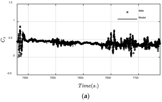

Figure 3.
Main aerodynamic coefficients predicted by the nonlinear and unsteady aerodynamic models. (a) Time history of normal force Cz; (b) Time history of pitching moment Cm; (c) Time history of rolling moment Cl; (d) Time history of yawing moment Cn.
The changes in the normal force coefficient (Cz) are large for both model predicted and input data before the modeling in Figure 3a due to the large variations in normal acceleration (az) and angle of attach (α), referred to in Figure 3a,b. The magnitudes of az and α (AOA) are obviously large to cause strong variations in the normal force coefficient (Cz) that started at roughly t = 7650 s.
The scattering of Cm data in Figure 3b is most likely caused by turbulence-induced buffeting [12,13] on the structure, particularly on the horizontal tail. The predicted results of others by the final models match well with the flight data. Once the aerodynamic models are set up, one can calculate all the necessary derivatives by a central difference scheme to analyze the stability characteristics.
The final main aerodynamic models of aerodynamic coefficients consist of many fuzzy rules for each coefficient, as described in Table 2 and Table 3. In Table 2 and Table 3, the numbers below each input variable represent the number of membership functions. The total number of fuzzy cells (n) in each model is the product of each number presented in column 3. The last column shows the final multiple correlation coefficients (R2). The accuracy of the established aerodynamic model through the fuzzy logic algorithm can be judged by the multiple correlation coefficients (R2).
Table 2.
Final main models of longitudinal aerodynamics.
Table 3.
Final main models of lateral-directional aerodynamics.
The twin-jet transport aircraft encountered clear-air turbulence during a commercial flight. As a result, several passengers and cabin crew members sustained injuries, and this event was classified as an aviation accident. To examine the dynamic stability characteristics, it is imperative to understand the flight environment in detail.
The corresponding flight data for twin-jet transport with plunging motion is presented in Figure 4. The dataset of the time span t = 7480~7739 s used for the modeling was extracted from the FDR. This twin-jet transport encounters severe clear-air turbulence twice during this time span. In Figure 4a, the variations in normal acceleration (az) show the highest az of 2.05 g around t = 7483 s and the lowest az of 0.08 g around t = 7484 s in the first turbulence encounter; in the second turbulence encounter, the highest az was 1.83 g around t = 7682 s and the lowest was 0.06 g around t = 7684 s. Figure 4b shows that the variation in α (AOA) is approximately in phase with az during those two turbulence encounters. The variation ranges of AOA are 4 deg. to −1.8 deg. in the first turbulence encounter and 5.5 deg. to −2 deg. in the second. The time history of β is about −2 deg. with the magnitude of small fluctuation, as indicated in Figure 4c. The aircraft rapidly plunges downward during the turbulence encounter. The largest drop-off height reaches 57.3 m in the time span t = 7484~7486 s. The Mach number (M) drops from 0.83 to 0.75 in the first turbulence encounter and from 0.80 to 0.70 in the second, as shown in Figure 4d.
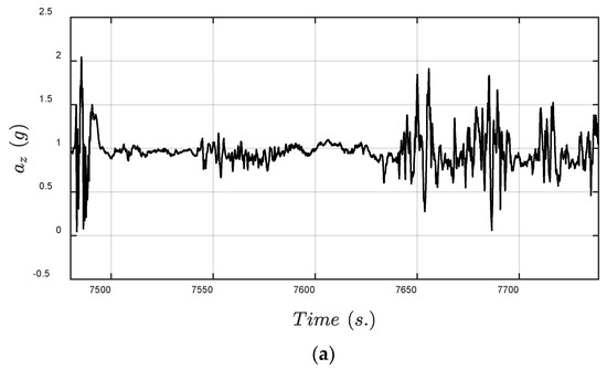
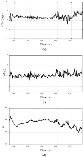
Figure 4.
Time history of main flight variables in severe clear-air turbulence. (a) Time history of normal acceleration (az); (b) Time history of angle of attack (AOA); (c) Time history of sideslip angle (β); (d) Time history of Mach number.
Figure 5 presents the twin-jet transport aircraft response to dynamic flight motion. The magnitudes of pitch rate (q) and roll rate (p) are shown in Figure 5a; the variation of p is larger than that of q. The yaw rate is not shown because it is small throughout. This implies that pitch angle (θ) does not vary as much as AOA and the variations in roll angle (ϕ) are large, especially during the second turbulence encounter.
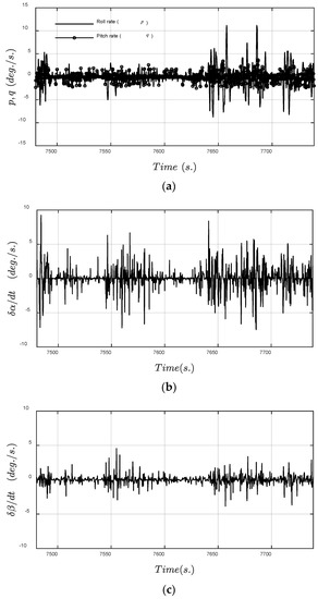
Figure 5.
Time history of twin-jet transport aircraft response to dynamic flight motion. (a) Time history of the pitch rate (q) and the roll rate (p); (b) Time history of the variable dα/dt; (c) Time history of the variable dβ/dt.
Figure 5b,c presents the time rate of the angle of attack (dα/dt, or ) and the time rate of the sideslip angle (), respectively. Figure 5b shows that variations in are approximately in phase with az and AOA during the two turbulence encounters. Figure 5c describes that the time history of β is about a certain value with the magnitude of small fluctuation. It implies that the twin-jet transport aircraft has a crosswind encounter, but this crosswind does not have variations in flight directions.
In general, the configuration of the static stability assessment is based on enough values of steady damping derivatives to maintain a stable condition. The longitudinal, roll, and directional damping derivatives have to be associated with - and - derivatives as oscillatory motion in a stability assessment. The longitudinal oscillatory derivatives are defined as [19]:
The roll and directional oscillatory derivatives are:
The values of oscillatory derivatives are equivalent to the combinations of steady damping and dynamic derivatives in Equations (38)–(41). The use of oscillatory derivatives instead of steady damping only is more consistent with the actual case of plunging motion. To be stable in oscillatory motion, (Czq)osc > 0, (Cmq)osc < 0, (Clp)osc < 0, and (Cnr)osc < 0. Physically, if it is unstable, the motion could be divergent in oscillatory motions within a short time period.
The (Czq)osc and (Cmq)osc would enlarge the variations in Cz and data scattering of Cm. The (Czq)osc and (Cmq)osc are insufficient in oscillatory damping, as shown in Figure 6a,b in the periods of t = 7484–7486 s and t = 7490–7494 s. The effect of -derivative on (Cmq)osc is to improve the stability in pitch in the periods of t = 7482.5–7484 s and 7486–7488.5 s. The values in the period of plunging motion have some differences between oscillatory and steady damping derivatives in Figure 6a,c due to the effects of the dynamic derivatives (i.e., -derivatives), and in Figure 7a,c due to the effects of the dynamic derivatives (i.e., -derivatives).
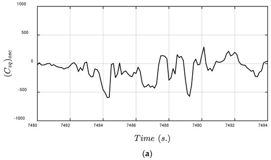
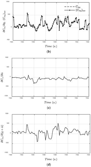
Figure 6.
Time history of main longitudinal oscillatory derivatives along the flight path. (a) Time history of (Czq)osc; (b) Time history of (Cmq)osc and Cmq; (c) The effects of -derivatives on Cz; (d) Time history of the dynamic derivatives of stability.
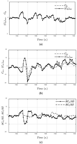
Figure 7.
Time history of main lateral-directional oscillatory derivatives along the flight path. (a) Time history of (Clq)osc and Clq; (b) Time history of (Cnr)osc and Cnr; (c) The effects of -derivatives on Cn and Cr.
Figure 6c,d and Figure 7c show dynamic derivatives of stability. To be stable, > 0, < 0, < 0, and > 0. The magnitudes of and have significant variations and < 0 in the period of t = 7482.5~7491 s in Figure 6b. It should be noted that represents the virtual mass effect and is particularly large in transonic flow to affect the plunging motion [28]. The magnitudes of in Figure 7c and (Clp)osc in Figure 7a are small; Clp is not shown because it is small throughout. The values of are from positive at t = 7483 s to negative at t = 7484 s; those of (Cnr)osc are from positive at t = 7483.5 s to negative at t = 7485 s. This implies that the effect of -derivative is to cause the directional stability to become more unstable.
In essence, the effects of -derivative on (Czq)osc and -derivative on (Clp)osc are small in Figure 6 and Figure 7. The effect of -derivative on (Cmq)osc is to improve the stability in pitch; the effect of -derivative is to cause more directional instability. These results indicate that the turbulent crosswind has some adverse effects on directional stability and damping. Although the dynamic derivatives tend to be small for the present configuration, these are helpful to understand the unknown factors of instability characteristics.
In the present study, the longitudinal and lateral-directional motion modes are analyzed based on the damping ratio (ζ) and undamped natural frequency (ωn). The roots of the complex conjugate are as follows:
where is a real part (i.e., in-phase) and are imaginary (i.e., out-of-phase) parts. λr and λi represent eigenvalues of real and imaginary parts, respectively. If λr is positive, the system is unstable; if it is negative, the system is stable [13].
Figure 8 presents the eigenvalues of the short-period and phugoid modes. The eigenvalues of the real part in Figure 8a are small negatives, except two portions at t = 7486.2 s and t = 7492.0–7493.0 s are small positives. The short-period mode is typically a damped oscillation in pitch about the body y-axis in normal flight conditions. The short-period mode is mostly in a stable condition due to the value of (Cmq)osc being mostly negative to have adequate pitch damping in oscillatory motions in the time span t = 7484–7486 s with largest drop-off height, the highest az being 2.05 g around t = 7483 s and the lowest being −1.05 g around t = 7484 s in Figure 4a, and the highest AOA being about 4 deg. in Figure 4b. The eigenvalues of the real part in Figure 8b are positive and the magnitude varies like a mountain chain with pinnacle. The value of (Czq)osc is negative and the magnitudes of also have negative values; (Czq)oscis insufficient in oscillatory damping with virtual mass effects during sudden plunging motion to cause the phugoid mode in an unstable condition. Note that part of the conventional phugoid mode has degenerated into the plunging mode.
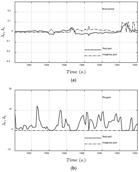
Figure 8.
Eigenvalues of longitudinal modes of motion. (a) The short-period mode; (b) The plunging mode.
Figure 9 presents the eigenvalues of the Dutch roll, spiral, and roll modes. The eigenvalues of the real part in Figure 9a are positive in the time period of t = 7490–7494 s and all values in Figure 9b are also positive, except the value of a small portion at t = 7484 s. The values of (Cnr)osc are mostly positive; (Cnr)osc is insufficient in oscillatory damping to induce the unstable Dutch roll and spiral modes. The eigenvalues of the real part in Figure 9c are negative. The roll mode is stable because the values of (Clp)oscare mostly small negatives to have some roll damping.
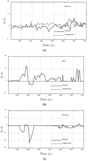
Figure 9.
Eigenvalues of lateral-directional modes of motion. (a) Eigenvalues of the Dutch roll mode; (b) Eigenvalues of the spiral mode; (c) Eigenvalues of the roll mode.
Airlines care about the vertical plunging mode of motion, which is not considered in classical flight dynamics. According to [28], in vertical plunging motion, the damping term is mainly related to . It may be possible to define the severity of plunging motion based on the vertical plunging equation of motion.
For the present purpose, if the severity is defined by the lowest load factor developed, this transport aircraft developed −1.05 g with Δh = 57.3 m (around t = 7483 s). The phugoid mode in Figure 8b has all positive real eigenvalues; this implies insufficient longitudinal oscillatory damping and virtual mass effects during sudden plunging motion. Thus, this transport does not have sufficient lateral-directional oscillatory damping. Therefore, it may be concluded that the plunging motion is more severe because of its unstable condition.
4. Concluding Remarks
The main objective of this paper was to present a dynamic stability monitoring method based on the approach of oscillatory motion and eigenvalue motion modes for jet transport aircraft response to sudden plunging motions. Three achievements can be concluded from the present paper as follows:
- (1)
- Flight data mining and fuzzy logic modeling were shown to be effective in establishing nonlinear and dynamic aerodynamic models through the flight data of FDR. The fuzzy logic aerodynamic models had robustness and nonlinear interpolation ability to generate the required independent variables in predicting the oscillatory motion during a severe clear-air turbulence encounter.
- (2)
- The eigenvalues of both longitudinal and lateral-directional motion modes were analyzed through digital flight simulation based on decoupled dynamic equations of motion. The decoupled concept is an innovative consideration for the flight simulation of 6-DOF.
- (3)
- The results of flight simulation showed that the phugoid, Dutch roll, and spiral modes were in unstable conditions for the transport aircraft examined in the present study. Those unstable conditions were easily judged by the positive real part of the eigenvalues during the sudden plunging motion.
The oscillatory motion and eigenvalue approaches for the dynamic stability assessments were helpful to understand the effects of severe clear-air turbulence encounters on dynamic stability characteristics. The simulated results could provide a training program of loss control prevention for airlines to enhance aviation safety and operational efficiency.
Author Contributions
Conceptualization, Y.W. and R.Z.; methodology, Y.W.; software, J.H., X.H. and J.Z.; validation, Y.W., F.Z., R.Z. and J.H.; investigation, Y.W., F.Z., J.H. and J.Z.; data curation, F.Z., R.Z., J.Z. and X.H.; writing—original draft preparation, Y.W., R.Z. and X.H.; writing—review and editing, Y.W. and R.Z.; funding acquisition, Y.W. All authors have read and agreed to the published version of the manuscript.
Funding
This research was supported in part by the Joint Funds Project of the National Natural Science Foundation of China (grant no. U1733203), the Special Key Projects of Technological Innovation and Application Development of Chongqing (grant no. cstc2019jscx-fxydX0036), the Scientific Research Project of CQJTU (grant no. 19JDKJC-A012), and the Research and Innovation Program for Graduate Students in Chongqing (2022S0085).
Institutional Review Board Statement
Not applicable.
Informed Consent Statement
Not applicable.
Data Availability Statement
Not applicable.
Conflicts of Interest
The authors declare no conflict of interest.
Nomenclature
| az | normal accelerations, g |
| b | wing span, m |
| Cx, Cz, Cm | longitudinal aerodynamic force and moment coefficients |
| Cy, Cl, Cn | lateral-directional aerodynamic force and moment coefficients |
| mean aerodynamic chord, m | |
| h | altitude, m |
| Ixx, Iyy, Izz | moments of inertia about x-, y-, and z-axes, respectively, kg∙m2 |
| Ixy, Ixz, Iyz | products of inertia, kg∙m2 |
| k1, k2 | longitudinal and lateral-directional reduced frequencies, respectively |
| M | Mach number |
| m | aircraft mass, kg |
| fuel flow rate, kg/hour | |
| N1 | the rpm of the compressor, rpm |
| p, q, r | Body axis roll rate, pitch rate, and yaw rate, deg./s |
| dynamic pressure, kpa | |
| S | wing reference area, m2 |
| T, W | thrust and aircraft weight in flight, N, respectively |
| T2 | time to double or halve the amplitude, s |
| t | time, s |
| X, Y, Z | forces acting on the aircraft body-fixed axes about x-, y-, and z-axes, respectively, N |
| α, | angle of attack, deg., and time rate of angle of attack, deg./s, respectively |
| β, | sideslip angle, deg., and time rate of sideslip angle, deg./s, respectively |
| δa, δe, δr | control deflection angles of aileron, elevator, and rudder, respectively, deg. |
| ϕ, θ, ψ | Euler angles in roll, pitch, and yaw, respectively, deg. |
| λr, λi | eigenvalue in real (i.e., in-phase) and imaginary (i.e., out-of-phase) parts, respectively |
| ζ | damping ratio |
| ωn | natural frequency |
| Abbreviations | |
| AAA | Advanced Aircraft Analysis |
| A/P | autopilot |
| DOF | degree of freedom |
| FDR | flight data recorder |
| FLM | Fuzzy logic modeling |
| IATA | International Air Transport Association |
References
- Chang, R.C.; Tan, S. Examination of dynamic aerodynamic effects for transport aircraft with hazardous weather conditions. J. Aeronaut. Astronaut. Aviat. 2013, 45, 51–62. [Google Scholar] [CrossRef]
- Sauer, M.; Steiner, M.; Sharman, R.D.; Pinto, J.O.; Deierling, W.K. Tradeoffs for routing flights in view of multiple weather hazards. J. Air Transp. 2019, 27, 70–80. [Google Scholar] [CrossRef]
- Hamilton, D.W.; Proctor, F.H. An aircraft encounter with turbulence in the vicinity of a thunderstorm. In Proceedings of the 21st AIAA Applied Aerodynamics Conference 2003, Orlando, FL, USA, 23–26 June 2003. [Google Scholar]
- Lee, Y.-N.; Lan, C.E. Analysis of random gust response with nonlinear unsteady aerodynamics. AIAA J. 2000, 38, 1305–1312. [Google Scholar] [CrossRef]
- Weng, C.-T.; Ho, C.-S.; Lan, C.E.; Guan, M. Aerodynamic analysis of a jet transport in windshear encounter during landing. J. Aircr. 2006, 43, 419–427. [Google Scholar] [CrossRef]
- Lan, C.E.; Chang, R.C. Unsteady aerodynamic effects in landing operation of transport aircraft and controllability with fuzzy-logic dynamic inversion. Aerosp. Sci. Technol. 2018, 78, 354–363. [Google Scholar] [CrossRef]
- Min, C.-O.; Lee, D.-W.; Cho, K.-R.; Jo, S.-J.; Yang, J.-S.; Lee, W.-B. Control of approach and landing phase for reentry vehicle using fuzzy logic. Aerosp. Sci. Technol. 2011, 15, 269–282. [Google Scholar] [CrossRef]
- Wang, Y.; Liu, P.; Hu, T.; Qu, Q. Investigation of co-rotating vortex merger in ground proximity. Aerosp. Sci. Technol. 2016, 53, 116–127. [Google Scholar] [CrossRef]
- Thompson, D.; Mogili, P.; Chalasani, S.; Addy, H.; Choo, Y. A computational icing effects study for a three-dimensional wing: Comparison with experimental data and investigation of spanwise variation. In Proceedings of the 42nd AIAA Aerospace Sciences Meeting and Exhibit, Reno, NV, USA, 5–8 January 2004; pp. 5470–5496. [Google Scholar]
- Lan, C.E.; Guan, M. Flight dynamic analysis of a turboprop transport airplane in icing accident. In Proceedings of the AIAA Atmospheric Flight Mechanics Conference 2005, San Francisco, CA, USA, 15–18 August 2005; pp. 551–569. [Google Scholar]
- Cabin Crew Turbulence Related Injuries, Safety Trend Evaluation. Analysis and Data Exchange System; Special Issue 2; IATA: Montreal, QC, Canada, 2005; pp. 19–22.
- Lan, C.E.; Chang, R.C. Fuzzy-Logic Analysis of the FDR Data of a Transport Aircraft in Atmospheric Turbulence; IntechOpen: London, UK, 2012; pp. 119–146. [Google Scholar]
- Chang, R.C.; Ye, C.-E.; Lan, C.E.; Guan, M. Flying qualities for a twin-jet transport in severe atmospheric turbulence. J. Aircr. 2009, 46, 1673–1680. [Google Scholar] [CrossRef]
- Wang, Y.; Chang, R.C.; Jiang, W. Assessment of flight dynamic and static aeroelastic behaviors for jet transport aircraft subjected to instantaneous high g-loads. Aircr. Eng. Aerosp. Technol. 2022, 94, 576–589. [Google Scholar] [CrossRef]
- Han, J.; Kamber, M.; Pei, J. Data Mining: Concepts and Techniques, 3rd ed.; Morgan Kaufmann Publishers: Burlington, MA, USA, 2011. [Google Scholar]
- FAA. Digital Flight Data Recorders for Transport Category Airplanes; FAR Part § 121.344; U.S. Department of Transportation: Washington, DC, USA, 2003.
- Wolberg, G.; Alfy, I. An energy-minimization framework for monotonic cubic spline interpolation. J. Comput. Appl. Math. 2002, 143, 145–188. [Google Scholar] [CrossRef]
- Lan, C.E.; Wu, K.; Yu, J. Flight Characteristics Analysis Based on QAR Data of a Jet Transport During Landing at a High-altitude Airport. Chin. J. Aeronaut. 2012, 25, 13–24. [Google Scholar] [CrossRef]
- Roskam, J. Airplane Flight Dynamics and Automatic Flight Controls; DARcorporation: Lawrence, KS, USA, 2018. [Google Scholar]
- Fazelzadeh, S.A.; Sadat-Hoseini, H. Nonlinear flight dynamics of a flexible aircraft subjected to aeroelastic and gust loads. J. Aerosp. Eng. 2012, 25, 51–63. [Google Scholar] [CrossRef]
- Chang, R.C. Performance diagnosis for turbojet engines based on flight data. J. Aerosp. Eng. 2014, 27, 9–15. [Google Scholar] [CrossRef]
- Chang, R.C.; Ye, C.-E.; Lan, C.E.; Guan, W.-L. Stability characteristics for transport aircraft response to clear-air turbulence. J. Aerosp. Eng. 2010, 23, 197–204. [Google Scholar] [CrossRef]
- Paziresh, A.; Nikseresht, A.H.; Moradi, H. Wing-Body and Vertical Tail Interference Effects on Downwash Rate of the Horizontal Tail in Subsonic Flow. J. Aerosp. Eng. 2017, 30, 04017001. [Google Scholar] [CrossRef]
- Hovanessian, S.A.; Pipes, L.A. Digital Computer Methods in Engineering; McGraw-Hill: New York, NY, USA, 1969. [Google Scholar]
- Karasan, A.; Ilbahar, E.; Cebi, S.; Kahraman, C. A new risk assessment approach: Safety and Critical Effect Analysis (SCEA) and its extension with Pythagorean fuzzy sets. Saf. Sci. 2018, 108, 173–187. [Google Scholar] [CrossRef]
- Dang, Q.V.; Vermeiren, L.; Dequidt, A.; Dambrine, M. Robust stabilizing controller design for TakagiSugeno fuzzy descriptor systems under state constraints and actuator saturation. Fuzzy Sets Syst. 2017, 329, 77–90. [Google Scholar] [CrossRef]
- Shi, K.; Wang, B.; Yang, L.; Jian, S.; Bi, J. TakagiSugeno fuzzy generalized predictive control for a class of nonlinear systems. Nonlinear Dyn. 2017, 89, 169–177. [Google Scholar] [CrossRef]
- Sheu, D.; Lan, C.-T. Estimation of turbulent vertical velocity from nonlinear simulations of aircraft response. J. Aircr. 2011, 48, 645–651. [Google Scholar] [CrossRef]


Publisher’s Note: MDPI stays neutral with regard to jurisdictional claims in published maps and institutional affiliations. |
© 2022 by the authors. Licensee MDPI, Basel, Switzerland. This article is an open access article distributed under the terms and conditions of the Creative Commons Attribution (CC BY) license (https://creativecommons.org/licenses/by/4.0/).