Autonomous Short-Term Traffic Flow Prediction Using Pelican Optimization with Hybrid Deep Belief Network in Smart Cities

Abstract

Accurate and timely traffic flow prediction not just allows traffic controllers to evade traffic congestion and guarantee standard traffic functioning, it even assists travelers to take advantage of planning ahead of schedule and modifying travel routes promptly. Therefore, short-term traffic flow prediction utilizing artificial intelligence (AI) techniques has received significant attention in smart cities. This manuscript introduces an autonomous short-term traffic flow prediction using optimal hybrid deep belief network (AST2FP-OHDBN) model. The presented AST2FP-OHDBN model majorly focuses on high-precision traffic prediction in the process of making near future prediction of smart city environments. The presented AST2FP-OHDBN model initially normalizes the traffic data using min–max normalization. In addition, the HDBN model is employed for forecasting the traffic flow in the near future, and makes use of DBN with an adaptive learning step approach to enhance the convergence rate. To enhance the predictive accuracy of the DBN model, the pelican optimization algorithm (POA) is exploited as a hyperparameter optimizer, which in turn enhances the overall efficiency of the traffic flow prediction process. For assuring the enhanced predictive outcomes of the AST2FP-OHDBN algorithm, a wide-ranging experimental analysis can be executed. The experimental values reported the promising performance of the AST2FP-OHDBN method over recent state-of-the-art DL models with minimal average mean-square error of 17.19132 and root-mean-square error of 22.6634.

1. Introduction

As a new form of intellectually complex mechanism, with high interaction and integration among multidimensional heterogeneous physical substances in network atmospheres [1,2], the cyber-physical system (CPS) compiles control, computing, and communication technologies to offer a practicable solution to and advanced technologies for the new generation of intelligent transportation system (ITS). This therefore is the key advancement direction of the CPS and resolves the issues of intellectual real-time target control and optimal dispatch of ITS [3]. Meanwhile, the issue of dense functions of large-scale data-computing and optimum control-scheduling methods in large-scale ITS is resolved by the speedy advancement of cloud computing (CC) technology. The basic principle of this was dispensing computing tasks on a great number of cloud-distributed computers; ITS management departments could then match CC sources to ITS cloud-controlled applications, evaluating storage systems and computers as required [4]. The implementation of CPS and CC technology makes it possible to attain, transfer and compute traffic data practically, and the implementation of the dynamic matrix method and artificial intelligence (AI) method could forecast traffic data in the next moment in advance [5].

Real-time precise short-time traffic flow forecasting could provide traffic guidance for traffic participants by selecting a suitable travel route, and aid the traffic controllers to have a fair control strategy for relieving traffic congestion [6]. Traffic flow becomes a time sequence data, having robust cyclicity and regularity that were considered as the base for precise estimation. However, its uncertainty and randomness raise prediction difficulties. Therefore, short-time traffic flow forecasting becomes necessary and challenging one in research domains and transport management [7]. Over the last few years, more techniques were deployed for forecasting short-term traffic flow, such as the autoregressive integrated moving average (ARIMA), fuzzy theory, artificial neural network (ANN), and Kalman filter. Such techniques proved to be helpful in deriving traffic flow temporary tendency and forecasting the future traffic flow. It was discovered from the literature that AI-related methods have been extensively utilized for object analytics and detection in ITS. However, such AI-enabled methods need precise perception [8]. However, prevailing approaches produce several mistakes at the time of execution, which may not applicable for realistic data analytics in ITS.

During the past few decades, several research proposals were suggested for enhancing self-learning approaches to dynamic and complex applications of the transport system [9]. Self-learning methods for traffic prediction could be widely split into 2 parts: nonparametric and parametric. In this context, a nonparametric method termed deep learning (DL) was found to be helpful for traffic flow forecasting with multidimensional features [10]. DL was a subset of machine learning (ML) that depends on the idea of deep neural network (DNN) and it was broadly utilized for object recognition, data classification, and natural language processing (NLP).

This manuscript introduces an autonomous short-term traffic flow prediction using an optimal hybrid deep belief network (AST2FP-OHDBN) model. The presented AST2FP-OHDBN model initially normalizes the traffic data using min–max normalization. In addition, the HDBN model is employed for forecasting the traffic flow in the near future, by the use of DBN with an adaptive learning step approach to enhance the convergence rate. To enhance the predictive accuracy of the DBN model, the pelican optimization algorithm (POA) is exploited as a hyperparameter optimizer, which in turn enhances the overall efficiency of the traffic flow prediction process. For assuring enhanced predictive outcomes of the AST2FP-OHDBN algorithm, a wide-ranging experimental analysis can be carried out.

2. Related Works

Zhang et al. [11] suggest a short-term traffic flow forecasting technique on the basis of a CNN-DL structure. In the presented structure, the optimum input duration lags and spatial data volumes were fixed by a spatio-temporal feature selection algorithm (STFSA), and the chosen spatio-temporal traffic flow features were derived from actual data and transformed into a 2-dimensional matrix. The CNN later studied such features for framing a predictive method. In [12], a hybrid technique compiling FNN and fuzzy rough set (FRS) can be suggested for imputation of missed traffic data. At first, FNN can be utilized for data classification; next, the KNN technique can be employed for determining optimal number of data leveraged to predict missing data in every category; lastly, the FRS was leveraged for imputing missed values. In [13], deep feature learning techniques were recommended for predicting short-term traffic flow in the succeeding multiple steps, utilizing supervised learning approaches. In order to reach traffic flow forecasting for the following day, an advanced multiobjective PSO method is implemented for optimizing certain variables in DBN. The modified method could foster the accuracy of the prediction fallouts and bolster their multiple step prediction capability.

Huang et al. [14] suggest a single-stage DNN-YOLOv3 (you only look once)-DL, that depends on the Tensorflow structure for improvising this issue. The network framework can be maximized by presenting the ideology of spatial pyramid pooling, afterward, the loss function was redefined, and a weight regularization technique was presented, in which, the statistics and real-time detections of traffic flow are applied efficiently. The optimization method uses the DL-CAR dataset for experimentations and end-to-end network training with datasets in various cases and weathers. In [15], a traffic flow detection method depending on DL on the edge node is suggested. Initially, the authors suggest a vehicle detection approach on the basis of the YOLOv3 method trained with a high volume of traffic data. They subsequently then pruned the method for ensuring competence on the edge equipment.

In [16], a novel end-to-end hybrid DL network method, termed M-B-LSTM, was suggested for short-term traffic flow forecasting in this work. In the M-B-LSTM method, online self-learning networks can be built as a data map layer for learning and equalizing the traffic flow statistic dispersal to reduce the impact of overfitting issues and distribution imbalance at the time of network learning. Feng et al. [17] suggest a new short-run traffic flow forecasting technique depends on an adaptive multikernel SVM (AMSVM) with spatial–temporal co-relation, termed AMSVM-STC. Initially, explore the randomness as well as nonlinearity of traffic flow, and hybrid polynomial kernel and Gaussian kernel for constituting the AMSVM. Secondly, the variables of AMSVM are optimized with the adaptive PSO method and recommends a new technique to constitute the hybrid kernel’s weight adjust adaptively in accordance with changing tendency of realistic traffic flow.

Xia et al. [18] presents a short-term traffic flow predictive approach which integrates community detection-based federated learning with graph convolutional network (GCN) for alleviating the time consuming trained, superior communication costs, and data privacy risks of global GCNs as the count of data improves. The federated community GCN (FCGCN) is attain accurate, timely, and safe traffic state predictive from the period of big traffic information that is an important for the effective function of intelligent transportation methods. Lin et al. [19] examines a process for screening spatial time-delayed traffic sequence dependent upon the maximal data coefficient. The selective time-delayed traffic sequence is changed as to traffic state vector in that traffic flow was predictive by implementing the integration of SVM and KNN techniques. The authors utilize the presented infrastructure to real-world traffic flow predictive. Chen et al. [20] introduces a new location GCN (Location-GCN). The location-GCN resolves this problem with added a novel learnable matrix as to GCN process, utilizing the absolute value of this matrix for representing the various control levels amongst distinct nodes. Afterward, the long short-term memory (LSTM) was utilized in the presented traffic predictive system. Besides, Trigonometric function encoder was utilized in this case for enabling the short-term input series for transferring the long-term periodical data.

3. The Proposed Model

Traffic flow prediction is developed by the use of present traffic data, past traffic data, and other related statistical data for establishing an appropriate mathematical method. An intellectual computation technique can be employed for making more accurate forecasting of traffic occurs in the upcoming years. The outcomes could offer a realistic foundation for vehicle dynamic guidance and urban traffic control. Assumes a provided time interval $t$ (i.e., every 15 min), $V\left(t\right)$ indicates the entire traffic data in time break. After, short run traffic flow forecasting issue solving methods in this study can be framed as follows. Presented a historical and present traffic data set $D=\left\{V\left(t\right), V \left(t-1\right), \dots , V\left(t-q\right)\right\}$, whereas t represents the current duration, q indicates time lag. The aim of short run traffic flow prediction was to forecast $Y=V\left(t+h\right)$, where $h \ge 1$ denotes the prediction horizon. For instance, $h=1$ means the predicted traffic flow at $t+1$. In this article, a new AST2FP-OHDBN technique was projected for traffic flow prediction in smart city environments. The presented AST2FP-OHDBN model employed min–max normalization to scale the input data and HDBN method can be employed for forecasting the traffic flow in the upcoming years. Finally, the POA is exploited as a hyperparameter optimizer which in turn enhances the overall efficiency of the traffic flow prediction process. Figure 1 depicts the overall process of proposed method.

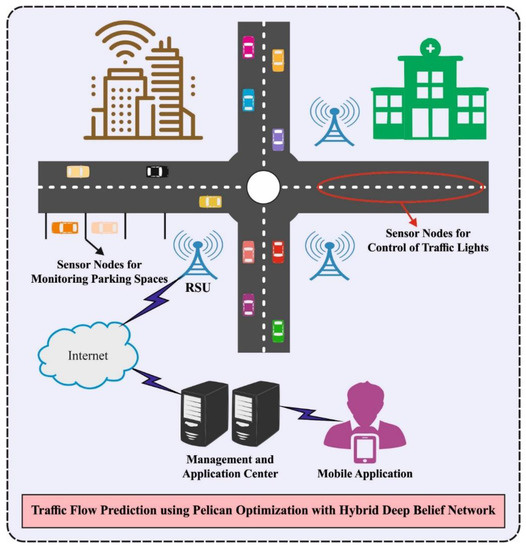
Figure 1. Overall process of proposed method.

3.1. Data Normalization

At the beginning level, the presented AST2FP-OHDBN model normalizes the traffic data using min–max normalization. The min–max method can be used in this work, given that the outcome of the linear transformation process of the original data comes up with the range of [0,1], as:

$$x_{scale}=\frac{x-x_{min}}{x_{max}-x_{min}}$$

(1)

where $x$ represents a recent value, $x_{min}$ and $x_{max}$ were the minimum and maximal value of the attributes, and $x_{scale}$ denotes the measure adjacent to the attribute matching processes.

3.2. Traffic Flow Prediction Using HDBN Model

For forecasting the traffic flow in the near future, the HDBN model is derived. DBN is a vital process from DL. Restricted Boltzmann Machine (RBM) unit is a generative stochastic artificial neural network which can learn a probability distribution over the set of inputs. It is similar to Boltzmann machines. It can be represented as the orientation of all actions and utilization of resources to accomplish effective results. The RBM improve the transparency and accountability, permitting intervention to complement each other and eliminate overlapping [21]. There is no linking amongst all the neural units from all the layers of RBM technique, besides, every neural unit from the visible layer (VL) was linked for every neural unit from the hidden layer (HL). Besides, the resultant of every layers of RBM was utilized as input for next layer. The bottom layer of DBN approach implements a multilayer RBM infrastructure. The greedy technique was utilized for training the instance data layer by layer. Figure 2 showcases the infrastructure of DBN. The DBN composed of multiple layers of latent variables (“hidden units”), with connections between the layers but not between units within each layer. The parameters attained with trained the primary layer RBM were utilized as input of secondary layer RBM, and the parameters of all the layers were attained by analogy. The trained procedure goes to unsupervised learning. The joint configuration energy of VL and HL in RBM are demonstrated as:

$$E\left(\nu , h|\theta \right)=-\sum _{i=1}^n{a}_i{v}_i-\sum _{j=1}^m{b}_i{h}_i-\sum _{i=1}^n\sum _{j=1}^m{v}_i{w}_{ij}{h}_j$$

(2)

where $\theta =\left\{w_{ij},a_i,b_j\right\}$, it can be linking weighted value amongst visible unit $i$ and hidden unit $j,$ $a_i$ refers the internal bias of VL neurons, and $b_j$ can be HLs. If the parameter $\theta$ is set, dependent upon the energy function, the joint probability distribution of VL and HL are attained in Equation (3) and linking it with Equation (4) as follows:

$$P\left(\nu , h|\theta \right)=\frac{e^{-E\left(v,h|\theta \right)}}{Z^{\theta }}$$

(3)

$$Z^{\theta }=\sum _{v,h}^{ }{e}^{-E(v,h|\theta )}$$

(4)

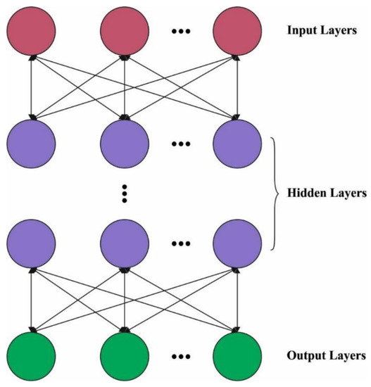
Figure 2. Structure of DBN.

If the state of VL $\nu$ is identified, the activation probability of $jth$ neural unit of HL $h$ is obtained:

$$P\left(h_j=1|\nu , \theta \right)=\sigma \left(b_j+\sum _i^{ }{v}_i{w}_{ij}\right)$$

(5)

If the HL state $h$ can be recognized, the activation probability of $ith$ neural unit of VL $\nu$ is reached:

$$P\left(v_i=1|h, \theta \right)=\sigma \left(a_i+\sum _i^{ }{h}_i{w}_{ij}\right)$$

(6)

In which, $\sigma \left(x\right)=\frac{1}{1+ \exp \left(-x\right)}$ refers the activation function, termed the sigmoid function. Every neuron is defining their state value as one or zero has probability $P$. For the unsupervised learning method, the drive of trained RBM can be obtaining the parameter method that is offered by log-likelihood function as:

$$L\left(\theta \right)=\sum _{n=1}^{N}ln\left(v^n,h\right)$$

(7)

$$\theta =argma\chi L\left(\theta \right)=argma\chi \sum _{n=1}^{N}ln\left(v^n,h\right)$$

(8)

The HDBN model is presented by the use of DBN with an adaptive learning step approach to enhance the convergence rate.

Training of the DBN model is difficult, especially in terms of training numerous RBMs. So, proper learning data requires fixing, which is essential to train the DBN model, by the use of contrastive divergence. A comparatively high learning rate results in unbalanced training procedure and low learning rate leads to a poor convergence rate. For addressing this issue, the HDBN model is derived using adaptive learning step (ALS) for computing effectual learning rate. The step size is modified based on the sign changes.

$$u{\gamma }_{ij}^{old}if\left({⟨{\nu }_i{h}_j⟩}_0-{⟨{\nu }_i{h}_j⟩}_k\right)({⟨{\nu }_i{h}_j⟩}_0^{old}-{⟨{\nu }_i{h}_j⟩}_0^{old})>0$$

(9)

$$d{\gamma }_{ij}^{old} if \left({⟨{\nu }_i{h}_j⟩}_0-{⟨{\nu }_i{h}_j⟩}_k\right)({⟨{\nu }_i{h}_j⟩}_0^{old}-{⟨{\nu }_i{h}_j⟩}_{\mathrm{k}}^{old})<0$$

(10)

where $u>1$ denotes incremental factor of learning step, $d<1$ defines decremental factor of learning step, ${\gamma }_{ij}^{old}$ was individual learning rate. If 2 consecutive upgrades were in the same direction, the step size would be increased and vice versa. The issues produced by inappropriate step size are evaded. In addition, convergence rate of the DBN method gets enhanced.

3.3. Hyperparameter Tuning

At the last stage, the POA is exploited as a hyperparameter optimizer, which in turn enhances the overall efficiency of the traffic flow prediction process. The presented POA is a population-based technique, whereas pelicans were members of this population [22]. For the population-based techniques, all the population members imply the candidate solutions. All the population members suggest values to optimize problem variables based on their place in relation to the searching space. Primarily, the population member is arbitrarily initialized based on the lower as well as upper bounds of the problem, utilizing Equation (11).

$$x_{i,j}=l_j+rand\cdot \left(u_j-l_j\right), i=1,2, \dots , N, j=1,2, \dots ,m,$$

(11)

where $x_{i,j}$ denotes the value of $jth$ variable detailed by the $ith$ candidate solution, $N$ represents the amount of population members, $m$ implies the amount of problem variables, $rand$ stands for the arbitrary number from interval of zero and one, $l_j$ refers the $jth$ lower bound, and $u_j$ represents the $jth$ upper bound of problem variables. The population members of pelicans from the presented POA were recognized utilizing a matrix, named as the population matrix in Equation (12). All the rows of this matrix signify the candidate solution, but the columns of this matrix signify the presented values for the problem variables.

$$X=\left[\begin{array}{l}{X}_1\hfill \\ ⋮\hfill \\ X_i\hfill \\ ⋮\hfill \\ X_N\hfill \end{array}\right] N\times m={\left[\begin{array}{ccccc}{\chi }_{1,1}\hfill & \dots & {\chi }_{1,j}& \dots & {\chi }_{1,m}\\ ⋮\hfill & \ddots & ⋮& & ⋮\\ {\chi }_{i,1}\hfill & \dots & {\chi }_{i,j}& \dots & {\chi }_{i_{,}m}\\ ⋮\hfill & & ⋮& \ddots & ⋮\\ x_{N,1}\hfill & \cdots & x_{N,j}& \dots & x_{N,m}\end{array}\right]}_{ N\times m}’$$

(12)

where $X$ refers to the population matrix of pelicans and $X_i$ denotes the $ith$ pelican. For the presented POA, all the population members are a pelican that is a candidate solution to the provided problem. Thus, the objective function of provided problem is estimated dependent upon all the candidate solutions. The value attained to objective function was defined utilizing a vector named the objective function vector in Equation (13).

$$F=\left[\begin{array}{l}{F}_1\hfill \\ ⋮\hfill \\ F_i\hfill \\ ⋮\hfill \\ F_N\hfill \end{array}\right] N\times 1^{=}{\left[\begin{array}{c}F\left(X_1\right)\\ ⋮\\ F\left(X_i\right)\\ ⋮\\ F\left(X_N\right)\end{array}\right]}_{ N\times 1}$$

(13)

In which $F$ stands for the objective function vector and $F_i$ represents the objective function value of $ith$ candidate solution.

The presented POA inspires the approach and behavior of pelicans if attack and hunt prey for updating the candidate solution. This hunting approach was inspired from 2 phases:

(i)

Moving to prey (exploration stage).

(ii)

Winging on the water surface (exploitation stage).

Exploration Phase

During the primary stage, the pelicans recognize the place of prey, and next moved to this recognized region. The pelican approach of moving to the place of prey was mathematically reflected in Equation (14).

$$x_{i,j}^{P_1}=\left\{\begin{array}{ll}{x}_{i,j}+rand\cdot \left(p_j-I\cdot x_{i,j}\right), \hfill & F_p<F_i,\hfill \\ x_{i,j}+rand\cdot \left(x_{i,j}-p_j\right),\hfill & else,\hfill \end{array}\right.$$

(14)

where $x_{i,j}^{P1}$ signifies the novel status of $ith$ pelican from the $jth$ dimensional dependent upon phase 1, $I$ signifies the arbitrary number that is equivalent to 1 or 2, $p_j$ represent the place of prey from the $jth$ dimensional, and $F_p$ is their objective function value. The parameter $I$ is a number which is arbitrarily equivalent to one or two. The upgrade procedure was modeled utilizing in Equation (15).

$$X_i=\left\{\begin{array}{l}{X}_i^{P_1}, F_i^{P_1}<F_{i;}\hfill \\ X_i, else,\hfill \end{array}\right.$$

(15)

In which $X_i^{P_1}$ demonstrates the novel status of $ith$ pelican and $F_i^{P_1}$ is their objective function value dependent upon stage 1.

Exploitation Phase

During the second stage, then the pelicans obtain the surface of water, it is spread its wings on the surface of water for moving the fish upwards, next gather the prey from its throat pouch. This approach leads additional fishes from the attacked region that caught by pelicans. The modeling this behavior of pelicans causes the presented POA for converging optimum points from the hunting region. This procedure enhances the local searching power and the exploitation capability of POA. In the mathematical approach, the technique must inspect the points from the neighborhood of pelican place for converging to an optimum solution. This behavior of pelicans in hunting was mathematically reflected in Equation (16).

$$x_{i,j}^{P_2}=x_{i,j}+R\cdot \left(1-\frac{t}{T}\right)\cdot \left(2\cdot rand-1\right)\cdot x_{i,j},$$

(16)

where $x_{i,j}^{P_2}$ signifies the novel status of $ith$ pelican from the $jth$ dimensional dependent upon stage 2, $R$ represents the constant that is equivalent to 0.2, $R\cdot \left(1-t/T\right)$ signifies the neighborhood radius of $x_{i,j}$ but, $t$ refers the iteration counter, and $T$ denotes the maximal amount of iterations. The coefficient “$R\cdot (1-t/T)$” implies radius of neighborhood of population members for searching locally neighboring all the members for converging to an optimum solution. During this stage, effectual upgrade is also utilized for accepting or rejecting the novel pelican place that is demonstrated in Equation (17).

$$X_i=\left\{\begin{array}{l}{X}_i^{P_2}, F_i^{P_2}<F_{i;}\hfill \\ X_i, else,\hfill \end{array}\right.$$

(17)

where $X_i^{P_2}$ refers the novel status of $ith$ pelican and $F_i^{P_2}$ is their objective function value dependent upon stage 2. Then, every population member is upgraded dependent upon the primary and secondary stages, dependent upon novel status of populations and the value of objective function, an optimum candidate solution so far is upgraded. This technique enters the next iteration and distinct steps of the presented POA dependent upon Equations (14)–(17) were repeating still the end of whole implementation. At last, an optimum candidate solution attained in the technique iterations is projected as a quasi-optimal solution to provided problem. The pseudocode of POA is given in Algorithm 1.

Algorithm 1: Pseudocode of POA.

1. Input

2. Computer POA population size (N) and iterations (T).

3. Initialize pelican location and determine objective function.

4. For $t=1:T$

5.     Produce prey location arbitrarily

6.     For $I=1:N$

7.     Stage 1: Move towards prey (exploration stage).

8.       For $j=1:m$

9.          Determine new position of the $jth$ dimension

10.        End.

11.       Upgrade the ith population member.

12.    Stage 2: Wing on water surface (exploitation stage).

13.       For $j=1:m.$

14.          Determine new status of the $jth$ dimension.

15.        End.

16.        Upgrade the ith population member.

17.     End.

18.     Upgrade optimal candidate solution.

19. End.

20. Output: Optimal candidate solution attained by POA.

End POA.

4. Results and Discussion

This section inspects the prediction performance of the AST2FP-OHDBN model in distinct aspects. The proposed model is tested by the traffic data containing all 30 s raw sensor data for a duration of 30 days. The traffic data collected during the first 10 days are used as a training set and the remaining 20 days data are utilized as testing set. In this experiment, data groups consist of the 15 min of aggregated data in vehicles per 15 min (veh per 15 min). Thereby, 96 data groups are available for each day. Before the calculation, the data groups are normalized (as given in Section 3.1), rendering the data in the range of 0 to 1.

Firstly, the mean absolute percentage error (MAPE) analysis of the proposed model is performed. The MAPE is a widely utilized measure for prediction process. It defines the ration of the sum of the individual absolute errors to the demand (each period separately). Table 1 and Figure 3 offer a detailed fitness value examination of the AST2FP-OHDBN model under varying numbers of iterations. The experimental values implicit in the AST2FP-OHDBN method have shown effectual outcomes with minimal fitness values. For instance, with 10 iterations, the AST2FP-OHDBN model has offered best, average, and worst fitness values of 1.996%, 5.237%, and 8.795% respectively. Meanwhile, with 50 iterations, the AST2FP-OHDBN method has provided best, average, and worst fitness values of 0.471%, 1.678%, and 5.046%, correspondingly. Eventually, with 100 iterations, the AST2FP-OHDBN technique has offered best, average, and worst fitness values of 0.471%, 1.013%, and 3.421%, correspondingly.

Table 1. MAPE analysis of AST2FP-OHDBN approach with distinct count of iterations.

MAPE (%)
No. of Iterations	Best Fitness	Average Fitness	Worst Fitness
0	10.828	11.051	10.987
10	1.996	5.237	8.795
20	0.884	3.140	7.302
30	0.471	1.075	5.046
40	0.471	1.583	4.506
50	0.471	1.678	5.046
60	0.471	1.170	4.283
70	0.471	1.138	3.521
80	0.471	1.774	3.870
90	0.471	1.774	3.743
100	0.471	1.013	3.421

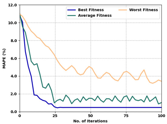
Figure 3. MAPE analysis of AST2FP-OHDBN approach with distinct count of iterations.

Table 2 and Figure 4 provide a detailed prediction results study of the AST2FP-OHDBN model under varying index. The experimental values highlighted the AST2FP-OHDBN method have attained closer predicted values under each run. For instance, on run-1 with an actual value of 190, the AST2FP-OHDBN model has attained the predicted value of 226. Moreover, on run-2 with an actual value of 190, the AST2FP-OHDBN method has reached the predicted value of 225. Furthermore, on run-3 with an actual value of 190, the AST2FP-OHDBN technique has gained the predicted value of 247. Finally, on run-5 with an actual value of 190, the AST2FP-OHDBN approach has reached the predicted value of 268.

Table 2. Traffic flow analysis of AST2FP-OHDBN approach with distinct runs.

Traffic Flow
Time Index	Actual	Predicted
		Run1	Run2	Run3	Run4	Run5
0	190	226	225	247	235	268
10	137	143	142	119	80	92
20	883	894	874	878	918	918
30	967	961	976	970	931	932
40	724	707	667	667	660	624
50	766	802	841	807	812	795
60	957	971	994	1003	980	945
70	844	860	832	842	875	902
80	973	1005	1031	1039	1003	1037
90	1030	1024	1032	1012	976	946
100	599	636	609	602	572	557

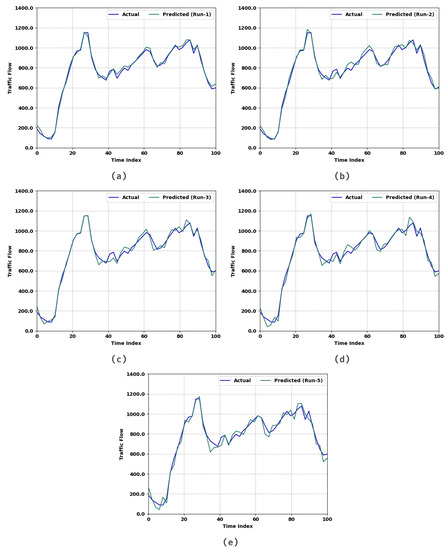
Figure 4. Traffic flow analysis of AST2FP –OHDBN approach (a) Run1, (b) Run2, (c) Run3, (d) Run4, and (e) Run5.

Table 3 demonstrates an extensive comparative study of the AST2FP-OHDBN model, with recent models given in terms of different measures [23]. Figure 5 illustrates a comparative scrutiny of the AST2FP-OHDBN method with existing methods in terms of RMSE. The figure represented the AST2FP-OHDBN technique has gained effectual outcomes over other models with minimal values of RMSE under all lags. For example, with lag = 1, the AST2FP-OHDBN technique has offered reduced RMSE of 26.9257. Conversely, the LS-SVM system, GA-LSSVM approach, PSO-LSSVM method, FFO-LSSVM technique, and hybrid LSSVM models have offered increased RMSE of 53.8171, 42.6758, 39.5084, 38.0203, and 32.7534 respectively. At the same time, with lag = 5, the AST2FP-OHDBN model has gained lower RMSE value of 23.4312. Conversely, the LS-SVM system, GA-LSSVM approach, PSO-LSSVM method, FFO-LSSVM technique, and hybrid LSSVM models have resulted in ineffectual outcomes with higher RMSE values of 98.8703, 58.9394, 55.5521, 53.4518, and 28.7079 respectively.

Table 3. Comparative analysis of AST2FP-OHDBN approach with existing methodologies under various measures.

No. of Lags	LS-SVM Model	GA-LSSVM	PSO-LSSVM	FFO-LSSVM	Hybrid-LSSVM	AST2FP-OHDBN
Root-Mean-Square Error
Lag = 1	53.8171	42.6758	39.5084	38.0203	32.7534	26.9257
Lag = 2	57.2355	46.9715	42.8572	41.0955	29.5013	23.6656
Lag = 3	61.4591	51.706	47.4003	45.2506	22.8315	16.5139
Lag = 4	95.8237	55.3336	51.0474	49.1178	27.9114	22.7806
Lag = 5	98.8703	58.9394	55.5521	53.4518	28.7079	23.4312
Mean Absolute Error
Lag = 1	38.3663	32.3363	24.7114	22.3607	21.8427	15.4770
Lag = 2	45.7351	39.6895	32.0517	25.2410	19.2498	12.3658
Lag = 3	51.3024	45.2973	39.4341	31.6977	23.5686	17.8232
Lag = 4	59.2069	51.9591	47.1757	37.1099	27.4439	20.5398
Lag = 5	67.0300	57.1088	52.4225	44.5820	24.4347	19.7508
Equal Coefficient
Lag = 1	0.9537	0.9557	0.9569	0.9579	0.9792	0.9835
Lag = 2	0.9518	0.9537	0.9555	0.9574	0.9788	0.9849
Lag = 3	0.9498	0.9513	0.9531	0.9543	0.9854	0.9877
Lag = 4	0.9482	0.9493	0.9513	0.9526	0.9839	0.9863
Lag = 5	0.9462	0.9477	0.9489	0.9507	0.9724	0.9861

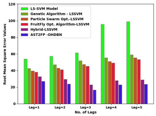
Figure 5. RMSE analysis of AST2FP-OHDBN approach with existing methodologies.

Figure 6 demonstrates a comparative inspection of the AST2FP-OHDBN approach with existing models in terms of MSE. The figure denoted the AST2FP-OHDBN method has gained effectual outcome over other models with minimal values of MSE under all lags. For example, with lag = 1, the AST2FP-OHDBN approach has rendered a reduced MSE of 15.4770. Conversely, the LS-SVM system, GA-LSSVM approach, PSO-LSSVM method, FFO-LSSVM technique, and hybrid LSSVM models have offered an increased MSE of 38.3663, 32.3363, 24.7114, 22.3607, and 21.8427, correspondingly. Meanwhile, with lag = 5, the AST2FP-OHDBN approach has acquired a lower MSE value of 19.7508. Conversely, the LS-SVM system, GA-LSSVM approach, PSO-LSSVM method, FFO-LSSVM technique, and hybrid LSSVM models have resulted in ineffectual outcomes with higher MSE values of 67.0300, 57.1088, 52.4225, 44.5820, and 24.4347, correspondingly.

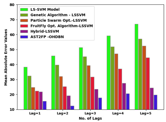
Figure 6. MSE analysis of AST2FP-OHDBN approach with existing methodologies.

A detailed equal coefficient (ECC) inspection of the results presented by the AST2FP-OHDBN model with existing models is given in Figure 7. The results demonstrated that the AST2FP-OHDBN model has attained enriched results, with higher values of ECC. For example, with lag = 1, the AST2FP-OHDBN method has reached increased ECC of 0.9835. Conversely, the LS-SVM system, GA-LSSVM approach, PSO-LSSVM method, FFO-LSSVM technique, and hybrid LSSVM models have obtained decreased ECC of 0.9537, 0.9557, 0.9569, 0.9579, and 0.9792 respectively. Likewise, with lag = 5, the AST2FP-OHDBN model has attained improved ECC of 0.9861. Conversely, the LS-SVM system, GA-LSSVM approach, PSO-LSSVM method, FFO-LSSVM technique, and hybrid LSSVM models have reached a reduced ECC of 0.9462, 0.9477, 0.9489, 0.9507, and 0.9724 respectively.

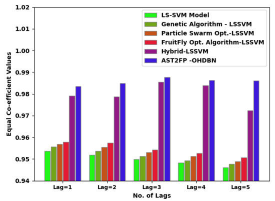
Figure 7. ECC analysis of AST2FP-OHDBN approach with existing methodologies.

Table 4 and Figure 8 depict a brief inspection of the AST2FP-OHDBN model with existing methods in terms of running time (RT). The figure implicit in the AST2FP-OHDBN model has acquired effectual outcomes over other models with minimal values of RT under all lags. For example, with lag = 1, the AST2FP-OHDBN model has provided a reduced RT of 3.84 s, whereas the LS-SVM system, GA-LSSVM approach, PSO-LSSVM method, FFO-LSSVM technique, and hybrid LSSVM models have offered increased RT of 7.26 s, 19.53 s, 11.29 s, 14.25 s, and 9.80 s, correspondingly.

Table 4. RT analysis of AST2FP-OHDBN approach with existing methodologies.

Running Time (sec)
No. of Lags	LS-SVM Model	Genetic Algorithm-LSSVM	Particle Swarm Opt.-LSSVM	FruitFly Opt. Algorithm-LSSVM	Hybrid-LSSVM	AST2FP-OHDBN
Lag = 1	7.26	19.53	11.29	14.25	9.80	3.84
Lag = 2	7.30	20.01	11.64	14.45	9.98	3.56
Lag = 3	7.42	20.33	11.67	15.06	10.02	5.13
Lag = 4	7.78	20.52	12.18	15.28	10.03	5.05
Lag = 5	7.89	22.00	12.24	15.31	10.44	5.07

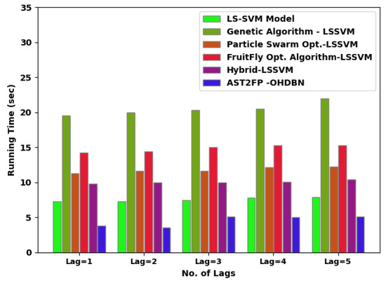
Figure 8. RT analysis of AST2FP-OHDBN approach with existing methodologies.

Simultaneously, with lag = 5, the AST2FP-OHDBN method has gained lower RT value of 5.07 s whereas the LS-SVM system, GA-LSSVM approach, PSO-LSSVM method, FFO-LSSVM technique, and hybrid LSSVM models have resulted in ineffectual outcomes with higher RT values of 7.89 s, 22 s, 12.24 s, 15.31 s, and 10.44 s, correspondingly. From the detailed result analysis, it is concluded that the AST2FP-OHDBN model has reached an effectual traffic flow forecasting performance.

5. Conclusions

In this article, a novel AST2FP-OHDBN model was projected for traffic flow prediction in smart city environments. The presented AST2FP-OHDBN model follows a three-stage process: min–max normalization, HDBN-based traffic flow forecasting, and POA-based hyperparameter tuning. Since the trial-and-error hyperparameter tuning of the HDBN model is a tedious process, the POA is applied as a hyperparameter optimizer, which considerable enhances the overall efficiency of the traffic flow prediction process. For assuring the enhanced predictive outcomes of the AST2FP-OHDBN algorithm, a wide-ranging experimental analysis can be executed. The experimental values reported the promising performance of the AST2FP-OHDBN model over recent state-of-the-art DL models with minimal average MSE of 17.19132 and RMSE of 22.6634. Therefore, the AST2FP-OHDBN algorithm can be employed to accomplish high-precision traffic prediction in the near future prediction on smart cities environment. In future, hybrid metaheuristics can be designed to enhance prediction outcomes.

References

- Nguyen, D.D.; Rohacs, J.; Rohacs, D. Autonomous flight trajectory control system for drones in smart city traffic management. ISPRS Int. J. Geo-Inf. 2021, 10, 338. [Google Scholar] [CrossRef]
- Cui, Q.; Wang, Y.; Chen, K.C.; Ni, W.; Lin, I.C.; Tao, X.; Zhang, P. Big data analytics and network calculus enabling intelligent management of autonomous vehicles in a smart city. IEEE Internet Things J. 2018, 6, 2021–2034. [Google Scholar] [CrossRef]
- Azgomi, H.F.; Jamshidi, M. A brief survey on smart community and smart transportation. In Proceedings of the 2018 IEEE 30th International Conference on Tools with Artificial Intelligence (ICTAI), Volos, Greece, 5–7 November 2018; IEEE: Piscataway, NJ, USA, 2018; pp. 932–939. [Google Scholar]
- Kuru, K.; Khan, W. A framework for the synergistic integration of fully autonomous ground vehicles with smart city. IEEE Access 2020, 9, 923–948. [Google Scholar] [CrossRef]
- Seuwou, P.; Banissi, E.; Ubakanma, G. The future of mobility with connected and autonomous vehicles in smart cities. In Digital Twin Technologies and Smart Cities; Springer: Cham, Switzerland, 2020; pp. 37–52. [Google Scholar]
- Chehri, A.; Mouftah, H.T. Autonomous vehicles in the sustainable cities, the beginning of a green adventure. Sustain. Cities Soc. 2019, 51, 101751. [Google Scholar] [CrossRef]
- Chen, X.; Chen, H.; Yang, Y.; Wu, H.; Zhang, W.; Zhao, J.; Xiong, Y. Traffic flow prediction by an ensemble framework with data denoising and deep learning model. Phys. A Stat. Mech. Its Appl. 2021, 565, 125574. [Google Scholar] [CrossRef]
- Zhou, T.; Han, G.; Xu, X.; Han, C.; Huang, Y.; Qin, J. A learning-based multimodel integrated framework for dynamic traffic flow forecasting. Neural Process. Lett. 2019, 49, 407–430. [Google Scholar] [CrossRef]
- Jia, T.; Yan, P. Predicting citywide road traffic flow using deep spatiotemporal neural networks. IEEE Trans. Intell. Transp. Syst. 2020, 22, 3101–3111. [Google Scholar] [CrossRef]
- Gu, Y.; Lu, W.; Xu, X.; Qin, L.; Shao, Z.; Zhang, H. An improved Bayesian combination model for short-term traffic prediction with deep learning. IEEE Trans. Intell. Transp. Syst. 2019, 21, 1332–1342. [Google Scholar] [CrossRef]
- Zhang, W.; Yu, Y.; Qi, Y.; Shu, F.; Wang, Y. Short-term traffic flow prediction based on spatio-temporal analysis and CNN deep learning. Transp. A Transp. Sci. 2019, 15, 1688–1711. [Google Scholar] [CrossRef]
- Tang, J.; Zhang, X.; Yin, W.; Zou, Y.; Wang, Y. Missing data imputation for traffic flow based on combination of fuzzy neural network and rough set theory. J. Intell. Transp. Syst. 2021, 25, 439–454. [Google Scholar] [CrossRef]
- Li, L.; Qin, L.; Qu, X.; Zhang, J.; Wang, Y.; Ran, B. Day-ahead traffic flow forecasting based on a deep belief network optimized by the multi-objective particle swarm algorithm. Knowl.-Based Syst. 2019, 172, 1–14. [Google Scholar] [CrossRef]
- Huang, Y.Q.; Zheng, J.C.; Sun, S.D.; Yang, C.F.; Liu, J. Optimized YOLOv3 algorithm and its application in traffic flow detections. Appl. Sci. 2020, 10, 3079. [Google Scholar] [CrossRef]
- Chen, C.; Liu, B.; Wan, S.; Qiao, P.; Pei, Q. An edge traffic flow detection scheme based on deep learning in an intelligent transportation system. IEEE Trans. Intell. Transp. Syst. 2020, 22, 1840–1852. [Google Scholar] [CrossRef]
- Qu, Z.; Li, H.; Li, Z.; Zhong, T. Short-term traffic flow forecasting method with MB-LSTM hybrid network. IEEE Trans. Intell. Transp. Syst. 2020, 23, 225–235. [Google Scholar]
- Feng, X.; Ling, X.; Zheng, H.; Chen, Z.; Xu, Y. Adaptive multi-kernel SVM with spatial–temporal correlation for short-term traffic flow prediction. IEEE Trans. Intell. Transp. Syst. 2018, 20, 2001–2013. [Google Scholar] [CrossRef]
- Xia, M.; Jin, D.; Chen, J. Short-Term Traffic Flow Prediction Based on Graph Convolutional Networks and Federated Learning. IEEE Trans. Intell. Transp. Syst. 2022, 1–13. [Google Scholar] [CrossRef]
- Lin, G.; Lin, A.; Gu, D. Using support vector regression and K-nearest neighbors for short-term traffic flow prediction based on maximal information coefficient. Inf. Sci. 2022, 608, 517–531. [Google Scholar] [CrossRef]
- Chen, Z.; Lu, Z.; Chen, Q.; Zhong, H.; Zhang, Y.; Xue, J.; Wu, C. A spatial-temporal short-term traffic flow prediction model based on dynamical-learning graph convolution mechanism. arXiv 2022, arXiv:2205.04762. [Google Scholar] [CrossRef]
- Li, F.; Zhang, J.; Shang, C.; Huang, D.; Oko, E.; Wang, M. Modelling of a post-combustion CO2 capture process using deep belief network. Appl. Therm. Eng. 2018, 130, 997–1003. [Google Scholar] [CrossRef]
- Trojovský, P.; Dehghani, M. Pelican optimization algorithm: A novel nature-inspired algorithm for engineering applications. Sensors 2022, 22, 855. [Google Scholar] [CrossRef] [PubMed]
- Luo, C.; Huang, C.; Cao, J.; Lu, J.; Huang, W.; Guo, J.; Wei, Y. Short-term traffic flow prediction based on least square support vector machine with hybrid optimization algorithm. Neural Process. Lett. 2019, 50, 2305–2322. [Google Scholar] [CrossRef]
Publisher’s Note: MDPI stays neutral with regard to jurisdictional claims in published maps and institutional affiliations. |
© 2022 by the authors. Licensee MDPI, Basel, Switzerland. This article is an open access article distributed under the terms and conditions of the Creative Commons Attribution (CC BY) license (https://creativecommons.org/licenses/by/4.0/).