Abstract
In this paper, the displacement fields responsible for acoustic emission (AE), excited from a point source in a transversely isotropic cylinder, are derived by solving the Navier-Lamé (NL) equation. The point source as an internal defect is represented by a spatiotemporal concentrated force. The introduction of three potentials correlated with the point source to displacement field vector decouples the coupled NL equation in cylindrical coordinates. Under these conditions, we solve the radial, tangential, and axial displacement fields. Analytical simulations of AE were carried out at several point source locations. Our results demonstrate that analytical modeling is a powerful tool for characterizing AE features generated from an internal defect source.
1. Introduction
Acoustic emission (AE) refers to the elastic wave generated by a material as a result of a sudden release of energy (other than heat) from localized sources within a solid. Material degradation related to deformation and fracture development is classified as the primary AE source, and is usually distinguished from secondary AE sources including leak and flow, chemical reactions, and the fabrication process. Crack formation and growth are the most important AE sources in practical non-destructive testing (NDT) investigations. The formation of a new crack face is accompanied by sudden changes in stress and displacement of the material in the vicinity of the crack. Consequently, an elastic wave is generated from the tip of the crack source [1]. AE testing has several unique advantages over other NDT methods, the most significant of which is its real-time monitoring capability; this allows for the detection of damage and degradation in various materials and structures [2,3,4,5,6]. AE data, refined with appropriate algorithms [7,8,9,10,11], provide useful information about the source of the emission and progression of crack growth; however, a quantitative interpretation of the AE signal is required to understand the physical processes underlying AE features. Analytical modeling of the AE signal is very important; however, in cylindrical structures, it is difficult to predict the AE generated from an internal crack.
The point source, defined as a body force f acting at a point, has been adapted as an AE excitation source in seismic displacements, crack formation and fracture, and concentrated vertical step force [12,13,14,15,16]. In the elastic field, the point source has been treated as a concentrated time harmonic source [17]. Although the AE generated by the point source is important for characterizing real signals observed in practical NDT investigations, theoretical modeling has been limited to spherical geometries with an infinite domain, given that a homogeneous solution is obtainable from the three-dimensional wave equation in spherical coordinates [12,13,17]. Most theoretical works on elastic wave propagation in cylindrical coordinates have focused on situations with or without external perturbations [18,19,20,21,22]. In cylindrical structures, the displacement field has been formulated in terms of one compression (P) potential, and two shear (vertically polarized, SV, and horizontally polarized, SH) potentials, by using the models proposed by Morse and Feshbach [23] and Buchwald [24], respectively. The basic difference between the two models is that the compression and shear parts are separated in one model, but not the other. The two models have been examined comprehensively by Honarvar et al. [18,19] and Sakhr et al. [21,22]. In contrast to cases that are unperturbed or perturbed by external forces, the three potentials should be incorporated along with the concentrated force (CF) exerted by the internal defects [17,25].
In this study, a “concentrated force-incorporated potential” (CFIP) is introduced into the displacement field on the basis of the model proposed by Morse and Feshbach [23], and the Navier-Lamé (NL) equation is constructed (which involves the CF in a transversely isotropic cylinder [TIC]). The CFIP allows the NL equation to be separated into three partial differential equations (PDEs), representing the potentials for P, SV, and SH waves. As an internal defect, the CF has both spatial and temporal properties, represented by the delta function and harmonic oscillation of the point source, respectively. For solving the NL equation, determining Green’s function for the delta function in cylindrical coordinates is the first task. Mohammad et al. proposed a Green’s function for a closed cylinder, using “the method of separation of variables” [26]. We reconstructed Green’s function for the delta function by applying the continuity and discontinuity principles to the boundary around the point source. Complete formation of the CF allowed us to solve the three potentials generated by the point source in the closed cylinder. Absolute values of the displacement fields were calculated by applying a fundamental set of boundary conditions in the cylinder to the solutions, in which two modes of CF along the radial and axial directions were considered. To our knowledge, no theoretical work on AE, excited by an internal point source in cylindrical geometries, has been presented in the literature. This paper establishes a mathematical model that provides insight into the overall process of the AE signal from generation and propagation to reception. These studies can be employed for evaluating the AE signal generated from an internal crack in a cylindrical structure.
2. Green’s Function
The body force arising from the point source located at is mathematically formulated in terms of an oscillating impulse with natural frequencies of the material in a given geometry, as follows:
where P(t) is the CF vector, is the delta function, and ω is the predominant angular frequency of AE. Green’s function , as the solution of the delta function, is defined as
The force can be rewritten as
In cylindrical coordinates, Equation (2) is expressed as
If , and ,
Green’s function is separable in a cylindrical coordinate system as
Substituting the Laplacian in cylindrical coordinates into Equation (5) gives the following:
Letting
then Equation (7) has the form
The solution of Equation (8) can be formulated in two regions:
The continuity and discontinuity principles are applied to find coefficients and . The continuity principle states that Green’s function is continuous around the point source, i.e.,
Equation (12) leads to
Although Green’s function is discontinuous at the point source, the difference in Green’s function between the adjacent two points, , around the point source is unity. When ε becomes 0, the discontinuity principle leads to
As a result, we obtain
From Equations (13) and (15),
Equation (11) becomes
The solution of Equation (9) can be written as
Applying the continuity principle to Equation (17) results in
The second restriction for is the symmetry between the point source and observation point, i.e.,
Equation (19) leads to
To satisfy the conservation law,
Equations (18) and (20) result in
For a complete cylinder, is periodic, with a period of 2π:
Therefore,
The final form of Equation (17) is
The solution of Equation (10) is a typical Bessel function, given by
where is the first kind of Bessel function of v-th order. Note that the second kind of Bessel function is excluded because it has a singularity at the origin, which is included in the domain of the cylinder. Applying the continuity principle to Equation (22), i.e., , results in
We find
where . In addition, applying the symmetry principle to Equation (22) gives , with
we obtain
Substituting Equations (23) and (24) into Equation (22) gives
Applying the boundary condition, i.e.,
to Equation (25) gives . Denoting the n-th root of the first kind of Bessel function of the v-th order as , i.e., , then . Since the first root of the first kind of Bessel function is most significant, we select n = 1.
Introducing a parameter, , to Equation (25) gives
From Equations (16), (21) and (27), the formula of the Green’s function for the Kronecker delta function becomes
The next task is to find the constant in Equation (28). Equation (4) is rewritten as
First, solve by integrating both sides over (0, l)
Therefore,
From Equations (16), (26), and (30), we obtain
and
Substituting Equation (21) into the above equation and integrating both sides over (0, 2π) gives
Since
the above equation is given by
Substituting Equation (27) into Equation (32) results in
Multiplying both sides of Equation (33) by and integrating over (0, ) gives
Given [26]
and
Equation (34) can be rewritten as
From Equation (35), we obtain the constant
Finally, we obtain the Green’s function for the Kronecker delta function
where
For an azimuthally independent force (v = 0), Equation (37) becomes
where
For convenience, we introduce new coordinates, defined as , and , where the location of the point source is the new origin at , and . Thus, Equations (39) and (40) are rewritten as
3. Displacement Fields Generated by a Point Source
The NL equation governing a wave in an elastic and homogeneous medium subject to a local body force f can be written in vector form, as follows [27]
where u is the displacement vector, λ and μ are the Lamé constants, and ρ is the density of the media. In this paper, the displacement field u in cylindrical coordinates proposed by Morse and Feshbach [23] is given as
where Φ is a scalar potential for the compressional wave (P), is a vector potential for the SH wave, is a vector potential for the SV wave, and a is the radius of the cylinder. When the displacement field is generated by an intrinsic point defect, the three potentials are correlated with the force vector P (referred to as CFIP) as
where ϕ, χ and ψ are unknown scalar functions, and the negative sign for the SH potential is used for further applications. Factoring the spatial and temporal parts in the potentials leads to
The displacement vector can be written as:
where , and . By substituting Equation (51) into Equation (43) and applying some manipulation, such as , , , and , Equation (43) can be rewritten as
In the above equation, the components in the gradient, the curl, and the curl of curl, can be independently zero
Introducing the longitudinal wave (P) speed and transverse wave (S) speed into the above equations leads to
where and , correspond to the angular wavenumbers of the P and the S waves, respectively. Taking into account the Laplacian operator in the cylindrical coordinates, the three scalar spatial potentials have the following forms:
First, let us solve PDE of Equation (56). Using a similar method to that applied to the case of Green’s function, the axial and the angular parts can be obtained as
respectively. Substituting the Laplacian operator and Equations (41), (59), (62), and (63), and introducing some straightforward algebra to Equation (56) leads to
where . Equation (64) is a second-order linear nonhomogeneous PDE, the solution of which is a linear combination of the homogeneous () and particular () solutions. The homogeneous solution of Equation (64) is
where and are the first kind and its modified Bessel functions, respectively, and and are the second kind and its modified Bessel functions, respectively. The Bessel functions of the second kind are excluded due to the singularity at the origin included in the domain of the cylinder. For the case of ,
According to Korenev’s solutions [28], the particular solution of the inhomogeneous equation has the form
The linear combination of Equations (65) and (66) results in
For further applications, the above equation is rewritten as
where the coupling constant .
Following a similar procedure, the functions of and can be obtained as
As shown in Figure 1, we introduce force vector P acting in the radial and the axial directions to solve for Φ. Equation (45) can be rewritten as
where , , and .
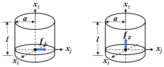
Figure 1.
Two forms of the point source vector along the xj and xz directions used in analytical modeling.
For ,
where
φ is the angle between an observation point and the axis.
For ,
By substituting Equation (67) into Equations (71) and (73), we obtain
In Equation (75),
From Equations (46) and (68), we obtain the SH potential:
For ,
In the above equation,
For ,
Similarly, for the SV potential, we find
All three potentials for the P, SH, and SV waves have now been completely determined, and we can thus derive the displacement components of and in terms of the three potentials. The relations between the displacements and potentials are given in Appendix A. First, let us derive the components generated by Pj. It can be easily shown that by substituting Equations (74), (77), and (80) into Equations (A5)–(A7), and taking the location of the point source as the origin , the displacement d component is reduced to
where subscript d represents the radial (r), the tangential (θ), or the axial (z) components.
For the radial component ,
For the tangential component ,
For the axial component ,
Following similar procedures, the three displacements generated by Pz can be derived by substituting Equations (75), (79), and (81) into Equations (A6)–(A8):
For the radial component ,
For the tangential component ,
For the axial component ,
The only remaining task to complete the displacement fields is to determine the coupling constants Am, Bm, and Cm. These constants can be determined directly by applying a fundamental set of linear elastic boundary problems. The outer surface of the cylinder studied in the present paper is stress-free. Thus, the following stress components are zero under these circumstances, i.e., :
Substituting Equations (A17)–(A21) into Equation (104) yields the following algebraic equations
where f = j for Pj and f = z for Pz. The elements in Equation (105) are given in Appendix A. For Pj, the elements of b1j, b2j and b3j are non-zero; therefore, the coupling constants can be determined by solving Equation (105).
The CF in Equations (1) and (43) is the force impulse defined as
where and b are parameters that determine the amplitude and the duration of the wave, respectively [29]. The arrival time τ of the impulse at the position must be considered, since the force impulse is acting in the f direction at position and at t = 0. Replacing t with (t − τ) yields
The displacement components generated by the potential, and the and potentials, correspond to the compressional (P), and the shear (SH and SV) waves, respectively; therefore, the arrival times of the two waves are given as
where and are the velocities of the P and S waves, respectively. The displacements generated by Pf can be rewritten as
Furthermore, the P, SH, and SV waves can be obtained from Equations (109)–(111) as
4. Simulation
In this study, we consider only the azimuthal dependence of the wave propagation arising entirely from the direction of the force vector, . A stainless-steel (SS) cylinder (a = 0.50 m, l = 2.0 m, ρ = 7.80 × 10³ kg/m3, km/s, and km/s) was used as the test specimen. Stiffness parameters ( can be found for austenitic stainless steel [30]. Previously, the natural frequencies of SS active on AE in the range of 0–300 kHz were determined experimentally by a tensile test (Appendix B). The frequency of ν = 155.4 kHz (the angular frequency ) was found to be predominant.
First, we determined by applying the boundary conditions to Equations (A20) and (A22) which were associated with the displacements due to . From Equation (105), two solutions of were obtained, as follows:
since .
When m = 0,
In Equations (117) and (119), the partial derivatives of with respect to η can easily be obtained from Equation (42). On the circumference, and , we solved the roots of the function
as a function of the shortest distance from the point source to the end plate of the cylinder (η) at a given . It should be noted that is independent of Ξ and Σ. Figure 2 shows the η dependence of three roots (n = 1–3) of Equation (120) for and 0.25 . In the simulation, we selected the first root (n = 1) at the given and values.
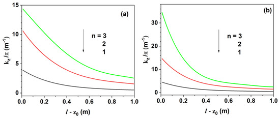
Figure 2.
Spectra of three sets of values calculated as a function of η(l − z0): (a) r0 = 0 and (b) r0 = 0.25 m .
Next, we determined P0 and b in Equation (107). The envelope of a given wave was evaluated by fitting its normalized form to determine b. As shown in Figure 3, when b = 6.0 × 10⁴ s−1, the duration (Δτ) of the wave was approximately 1 ms. By increasing the b value, the duration of the envelope decreased exponentially at b = 4.0 × 10⁵ s−1 with Δτ ≅ 25 μs. In the simulation, the force exerted by the point source was fixed to 1 N with P0 = 1.0 × 10¹⁰ N s−1 and b = 1.0 × 10⁵ s−1.
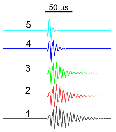
Figure 3.
Effect of the b parameter of the point source on the envelopes of the simulated waveforms: (1) 6 × 10⁴, (2) 8 × 10⁴, (3) 1 × 10⁵, (4) 2 × 10⁵, and (5) 4 × 10⁵.
In the simulation two positions of the point source of 1 N were considered, with coordinates of (0 m, 0 m, 1 m) and (0 m, 0.25 m, 1 m). Figure 4a shows the displacements, and their wave properties, at the (0.5 m, 45°, 1 m) position, generated by the point source located at the center of the cylinder (0 m, 0 m, 1 m). The Pj excitation produces an axial displacement that is stronger than the radial and tangential displacements. These displacements result in the P wave being the main wave, with a minor SH wave and very weak SV wave (Figure 4b). As shown in Figure 4c, the displacement features generated by the Pz excitation differ significantly from those generated by the Pj excitation. For the Pj excitation, the maximum values of and at the (0.5 m, 45°, 1 m) position were 0.29 and 0.71 nm, respectively, whereas for the Pz excitation, they were 28.1 and 5.0 nm, respectively. The amplitudes of the displacements due to the Pz excitation were much stronger than those due to the Pj excitation. It should be noted that the Pz excitation produces only the P wave (Figure 4d). The angular dependence of the displacement was also calculated (Figure 5). When the point source is located at the center of the circular plane, the angular dependences of , and arise from only Ξ and Σ as defined in Equations (72) and (78), respectively. For Pz excitation, the displacements of and are free from these factors. When the distances from the point source to the circumference are not equivalent, the angular dependences of the radial and axial displacements are highly significant. These effects are due not only to Ξ and Σ but also the superposition of the Bessel functions involved in the displacement equations. At a certain angle, some values in Equation (105) become too small to cause the sudden increase in displacement.
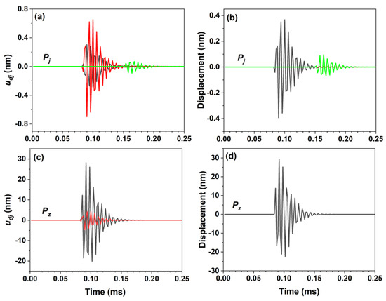
Figure 4.
Displacements at the (0.5 m, 45°, 1 m) position generated by the point source of 1.0 N located at the center of the cylinder: (a,c) radial (black line), axial (red line), and tangential (green line) components; and (b,d) compression P (black line) wave and vertically polarized (SV, red line) and horizontally polarized (SH, green line) shear waves.
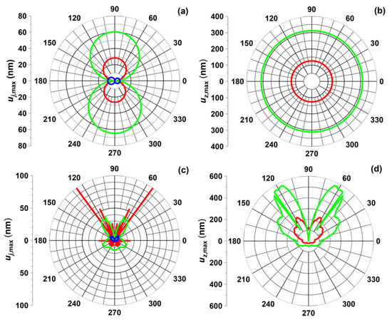
Figure 5.
Angular dependences of the maximum displacements at the (0.5 m, 45°, 1 m) position: radial (red line), axial (green line), and tangential (blue line) displacements generated by (a,c) Pj and (b,d) Pz of 1.0 N, located at (a,b) (0 m, 0 m, 1 m) and (c,d) (0 m, 0.25 m, 1 m) positions.
5. Conclusions
In this paper, we present a mathematical model for AE generated by a point source in a TIC. The point source as the CF vector is a model for an initiation state of crack formation in a solid medium. In the cylindrical system, the displacement field vector is very complex: compressional (P), and vertical and horizontal shear (SV and SH) wave potentials are coupled. Introducing CFIPs into the NL equation leads to the solutions of the radial, tangential, and axial displacements in the cylindrical system. The solutions obtained in this study can be used for analyzing experimental data for the NDT of cylinders. In the near future, similar mathematical models will be developed for shells and multilayered cylinders.
Author Contributions
Conceptualization, methodology and investigation, K.B.K. and J.-G.K.; software, validation, and formal analysis, K.B.K.; resources and data curation, S.G.L.; writing—original draft preparation, K.B.K. and J.-G.K.; writing—review and editing, visualization, and supervision, J.-G.K.; project administration and funding acquisition, B.K.K. All authors have read and agreed to the published version of the manuscript.
Funding
This research was funded by the Korea Institute of Energy Technology Evaluation and Planning (KETEP) and the Ministry of Trade, Industry & Energy (MOTIE) of the Republic of Korea (NO. 20202910100070).
Institutional Review Board Statement
Not applicable.
Informed Consent Statement
Not applicable.
Data Availability Statement
Not applicable.
Conflicts of Interest
The authors declare no conflict of interest.
Appendix A
Some gradient, divergence and curl operators on the potentials are as follows:
Substituting the above equations into Equation (44) gives
From Equation (A5), we obtain the displacement components as
in which ur, uθ and uz denote the radial, tangential, and axial displacements, respectively. The radial component can be obtained by substituting Equations (71), (77), and (79) into Equation (A6) in the coordinates.
where and . By rearranging the above equation in terms of the Am, Bm and Cm coupling constants, we obtain
where
For TIC, the stress-strain [18] and the strain-displacement [31] relations are given as
and
respectively. From these relations, one can obtain three stresses of , and as [18]:
From , and
where
where
and
where
From , and
where
where
and
where
Appendix B
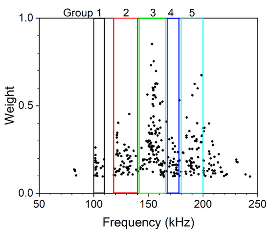
Figure A1.
Distribution of resolved frequency components and the 5 groups selected using a 10 kHz wide window. The experimental data are obtained from a tensile test using AISI 316 austenitic stainless steel (KS D 3698 standard).

Table A1.
Resolved frequency components (ν’s) and their relative weights of 316 stainless steel.
Table A1.
Resolved frequency components (ν’s) and their relative weights of 316 stainless steel.
| Group | Elements a | ν/kHz b |
|---|---|---|
| 1 | 20(0.07) | 103.2(2.62) |
| 2 | 58(0.21) | 127.6(5.59) |
| 3 | 114(0.41) | 155.4(5.37) |
| 4 | 36(0.13) | 173.6(3.28) |
| 5 | 51(0.18) | 190.6(4.72) |
a Value in parenthesis represents the fraction. b Value in parenthesis represents the standard deviation.
References
- Seruby, C.B. An Introduction to acoustic emission. J. Phys. E Sci. Instrum. 1987, 20, 946–953. [Google Scholar]
- Godin, N.; Reynaud, P.; Fantozzi, G. Challenges and Limitations in the Identification of Acoustic Emission Signature of Damage Mechanisms in Composites Materials. Appl. Sci. 2018, 8, 1267. [Google Scholar] [CrossRef] [Green Version]
- Domaneschi, M.; Niccolini, G.; Lacidogna, G.; Cimellaro, G.P. Nondestructive Monitoring Techniques for Crack Detection and Localization in RC Elements. Appl. Sci. 2020, 10, 3248. [Google Scholar] [CrossRef]
- Oh, T.-M.; Kim, M.-K.; Lee, J.-W.; Kim, H.; Kim, M.-J. Experimental Investigation on Effective Distances of Acoustic Emission in Concrete Structure. Appl. Sci. 2020, 10, 6051. [Google Scholar] [CrossRef]
- Goldaran, R.; Turer, A.; Kouhdaragj, M.; Ozlutas, K. Identification of Corrosion in a Prestressed Concrete Pipe Utilizing Acoustic Emission Technique. Constr. Build. Mater. 2020, 242, 118053. [Google Scholar] [CrossRef]
- Dong, L.; Tong, X.; Ma, J. Quantitative Investigation of Tomographic Effects in Abnormal Regions of Complex Structures. Engineering 2021, 7, 1011–1022. [Google Scholar] [CrossRef]
- Chai, S.; Zhang, Z.; Duan, Q. A New Qualitative Acoustic Emission Parameter Based on Shannon’s Entropy for Damage Monitoring. Mech. Syst. Signal Process. 2018, 100, 617–629. [Google Scholar] [CrossRef]
- Krampikowska, A.; Pała, R.; Dzioba, I.; Świt, G. The Use of the Acoustic Emission Method to Identify Crack Growth in 40CrMO Steel. Materials 2019, 12, 2140. [Google Scholar] [CrossRef] [Green Version]
- Kovač, J.; Legat, A.; Zajec, B.; Kosec, T.; Govekar, E. Detection and Characterization of Stainless Steel SCC by the Analysis of Crack Related Acoustic Emission. Ultrasonics 2015, 62, 312–322. [Google Scholar] [CrossRef] [Green Version]
- Kek, T.; Kusič, D.; Svečko, R.; Hančič, A.; Grum, J. Acoustic Emission Signal Analysis for the Integrity Evaluation. J. Mech. Eng. 2018, 64, 665–671. [Google Scholar]
- Mukherjee, A.; Banerjee, A. Analysis of Acoustic Emission Signal for Crack Detection and Distance Measurement on Steel Structure. Acoust. Aust. 2021, 49, 133–149. [Google Scholar] [CrossRef]
- Aki, K.; Richards, P.G. Quantitative Seismology, 2nd ed.; University Science Books: Mill Valley, CA, USA, 2009; Chapter 4. [Google Scholar]
- Pujol, J.; Herrmann, B. A Student’s Guide to Point Sources in Homogeneous Media. Seismolog. Res. Lett. 1990, 61, 209–221. [Google Scholar] [CrossRef]
- Scruby, C.B.; Wadley, H.N.G.; Hill, J.J. Dynamic Elastic Displacements at the Surface of an Elastic Half-space due to Defect Sources. J. Phys. D Appl. Phys. 1983, 16, 1069–1083. [Google Scholar] [CrossRef]
- Ohtsu, M.; Ono, K. The Generalized Theory and Source Representation of Acoustic Emission. J. Acoust. Emiss. 1986, 5, 124–133. [Google Scholar]
- Weaver, R.L.; Pao, Y.-H. Axisymmetric Elastic Waves Excited by a Point Source in a Plate. J. Appl. Mech. 1982, 49, 821–836. [Google Scholar] [CrossRef]
- Mal, A.K.; Singh, S.J. Deformation of Elastic Solids; Prentice Hall: New York, NY, USA, 1991; pp. 312–317. [Google Scholar]
- Honarvar, F.; Sinclair, A.N. Acoustic Wave Scattering from Transversely Isotropic Cylinders. J. Acoust. Soc. Am. 1996, 100, 57–63. [Google Scholar] [CrossRef]
- Honarvar, F.; Enjilela, E.; Sinclair, A.N.; Mirnezami, S.A. Wave Propagation in Transversely Isotropic Cylinders. Int. J. Solids Struct. 2007, 44, 5236–5246. [Google Scholar] [CrossRef] [Green Version]
- Ponnusamy, P.; Selvamani, R. Wave Propagation in a Homogeneous Isotropic Cylindrical Panel. ATAM 2011, 2, 171–181. [Google Scholar]
- Sakhr, J.; Chronik, B.A. Solving the Navier-Lamé Equation in Cylindrical Coordinates using the Buchwald Representation: Some Parametric Solutions with Applications. Adv. Appl. Math. Mech. 2018, 10, 1025–1056. [Google Scholar]
- Sakhr, J.; Chronik, B.A. Constructing Separable non-2π-Periodic Solutions to the Navier-Lamé Equation in Cylindrical Coordinates using the Buchwald Representation: Theory and Applications. Adv. Appl. Math. Mech. 2020, 12, 694–728. [Google Scholar]
- Morse, P.M.; Feshbach, H. Methods of Theoretical Physics; McGraw-Hill: New York, NY, USA, 1953; pp. 1764–1767. [Google Scholar]
- Buchwald, V.T. Rayleigh Waves in Transversely Isotropic Media. Q. J. Mech. Appl. Math. 1961, 14, 293–317. [Google Scholar] [CrossRef]
- Kund, T. Mechanics of Elastic Waves and Ultrasonic Nondestructive Evaluation; CRC Press: Boca Raton, FL, USA, 2019; pp. 76–78. [Google Scholar]
- Nezhad Mohammad, A.M.; Abdipour, P.; Bababeyg, M.; Noshad, H. Derivation of Green’s Function for the Interior Region of a Closed Cylinder. Amirkabir Int. J. Sci. Res. 2014, 46, 23–33. [Google Scholar]
- Eringen, A.C.; Suhubi, E.S. Fundamentals of Linear Elastodynamics. In Elastodynamics; Academic Press: New York, NY, USA, 1975; Volume II, pp. 343–366. [Google Scholar]
- Korenev, B.G. Bessel Functions and Application; Taylor & Francis: New York, NY, USA, 2002; p. 55. [Google Scholar]
- Hora, P.; Červená, O. Acoustic Emission Source Modeling. Appl. Comput. Mech. 2010, 4, 25–36. [Google Scholar]
- Dou, Y.; Luo, H.; Zhang, J. Elastic Properties of FeCr20Ni8Xn (X = Mo, Nb, Ta, Ti, V. W and Zr) Austenitic Stainless Steels: A First Principles Study. Metals 2019, 9, 145. [Google Scholar] [CrossRef] [Green Version]
- Boresi, A.P.; Chong, K.P.; Lee, J.D. Elasticity in Engineering Mechanics, 3rd ed.; John Wiley & Sons: Hoboken, NJ, USA, 2011; pp. 150–151. [Google Scholar]
Publisher’s Note: MDPI stays neutral with regard to jurisdictional claims in published maps and institutional affiliations. |
© 2022 by the authors. Licensee MDPI, Basel, Switzerland. This article is an open access article distributed under the terms and conditions of the Creative Commons Attribution (CC BY) license (https://creativecommons.org/licenses/by/4.0/).