Article

A Model Test of the Dynamic Stiffnesses and Bearing Capacities of Different Types of Bridge Foundations

1
Railway Engineering Research Institute, China Academy of Railway Sciences Corporation Limited, Beijing 100081, China
2
State Key Laboratory of High Speed Railway Track Technology, China Academy of Railway Sciences Corporation Limited, Beijing 100081, China
3
School of Civil Engineering, Beijing Jiaotong University, Beijing 100044, China
*
Author to whom correspondence should be addressed.
Appl. Sci. 2022, 12(10), 4951; https://doi.org/10.3390/app12104951
Submission received: 31 March 2022 / Revised: 12 May 2022 / Accepted: 12 May 2022 / Published: 13 May 2022
(This article belongs to the Special Issue Geotechnical Testing Technology: Development and Applications)

Abstract

:
With the rapid development of traffic infrastructures in developing countries, the evaluation demands for the vertical capacities of in-service bridges are increasing. The feasibilities of the transient response method (TRM) and index of dynamic stiffness for evaluating pile foundations are proven. However, their applicability to other types of bridge foundations must be investigated, and the correlation between the dynamic and static stiffnesses is also needed for analysis. In the present study, model tests were performed in a laboratory for various types of bridge foundations. A total of eight foundation models were fabricated for three types of bridge foundations. Both TRM and static loading tests were applied on each model. The influence of the foundation constraint state was tested as well. The results show that there is an obvious correlation between the dynamic and static stiffnesses and that the index of dynamic stiffness can reflect the foundation bearing capacity. Accordingly, the TRM can be employed to evaluate different foundation types, including spread, caisson, and pile foundations.

1. Introduction

With the rapid development of traffic infrastructures in developing countries over the last two decades, the demands for the bridge maintenance, disease diagnosis, and reinforcement are increasing [1,2]. Unlike the bridge superstructures, the pier foundations are buried in the ground, and the disease degree and its location cannot be identified by conventional detection methods. Hence, it is more difficult to quantitatively evaluate the bearing capacities of such foundations [3,4,5,6]. In real bridge foundations, it is always a combination of vertical, longitudinal, and lateral forces. The bridge dynamic problem under the action in the horizontal direction has been widely investigated, e.g., under seismic excitation and scour [7,8,9,10]. The effect on the lateral state can be directly inspected using diving underwater observation and direct observation during dry periods [11,12]. The dynamic method can also be used to evaluate the later condition of bridge substructures [13,14]. However, as the train loads mainly provide the quasi-static load and parameter excitations in the vertical direction [15,16,17,18], when the freight volume or train speed is required to be increased, the associated increase in the axle loads has the potential effect on the vertical bearing capacity of bridge substructures. Thus, the capacities of bridge substructures need to be estimated [19]. To obtain the actual foundation bearing capacity in the vertical direction, the most widely used method is the static loading test (SLT), which is also a typical static method to test the capacities of buildings and bridge foundation piles [20,21,22]. Wang et al. (2016) [23] discussed different prediction methods for the bearing capacities of piles. Zhang et al. (2016) [24] presented an analytical method to assess the influences of reaction piles on the test pile responses in SLT. Baca et al. (2020) [25] examined a new method of bi-directional SLT in the laboratory using six model piles. In addition to the SLT, dynamic testing can also be employed to estimate the pile capacity. The high-strain dynamic pile testing (HSDPT) method is generally used to evaluate the capacity of a deep foundation [26,27]. However, both SLT and HSDPT are difficult to use on existing bridge foundations that are in service, as permanent displacements can be generated by these methods.
For bridges with potential diseases or for bearing increasing train loads and train speeds, it is considered significant that engineers learn the real foundation capacities to determine whether the foundations need to be strengthened. Then, the transient response method (TRM) and index of dynamic stiffness (Kd) are proven to be feasible. The TRM is also known as the mechanical mobility method. By applying a vertical impact load on the foundation, both the velocity responses and force signals can be analysed in the frequency domain. The mechanical admittance spectrum or mobility can be obtained using the velocity and force spectra [28]. Using the TRM, the dynamic stiffness can be obtained as follows [29,30,31]:
K d ( f ) = 2 π f | V ( f ) / F ( f ) | ,
where V(f) is the Fourier spectrum of the velocity response v(t), F(f) is the Fourier spectrum of the force F(t), and the ratio of V(f)/F(f) is the mechanical admittance spectrum or velocity mobility [28]. Figure 1 shows the theoretical velocity mobility of a pile obtained using the TRM. In the low-frequency range, the ideal velocity mobility varies linearly with the frequency; accordingly, the value of Kd in the low-frequency range is a constant.
Recently, the TRM and Kd were employed for pile foundation evaluations. Liu and Ma [32] proved that in the pile capacity estimation, a reasonable value of Kd could be employed as an alert value. Ma et al. [33] indicated that Kd could be employed to estimate the pile bearing capacity. Chu et al. [34] investigated the influence of the cap–pile system on Kd. Liu and Ma [35] performed both TRM and SLT on a full-scale pier–cap–pile system and analysed the relationship between the dynamic stiffness and foundation capacity. However, the above studies only analysed the applicability of the TRM to pile foundations; other types of bridge foundations, such as the widely used spread foundation and caisson foundation, were not considered. In addition, most studies have only considered the TRM; a few tests were reported on the use of both TRM and SLT on the same foundation because of low feasibility of the SLT to evaluate in-service pier foundations and the associated high testing cost. If the TRM and Kd are used to evaluate the capacities of different types of bridge foundations, then the relationships between the dynamic stiffnesses and bearing capacities could be further investigated. Therefore, in this study, a model test was performed in the laboratory, where both the TRM and SLT were used to assess three types of bridge foundations: spread, caisson, and grouped pile foundations. The dynamic stiffnesses were analysed when the foundations were first fully buried in the soils and then when the constraint states were changed. Subsequently, the static stiffnesses were calculated using the SLT results. Finally, the relationship between the dynamic and static stiffnesses was analysed.

2. Test Outline

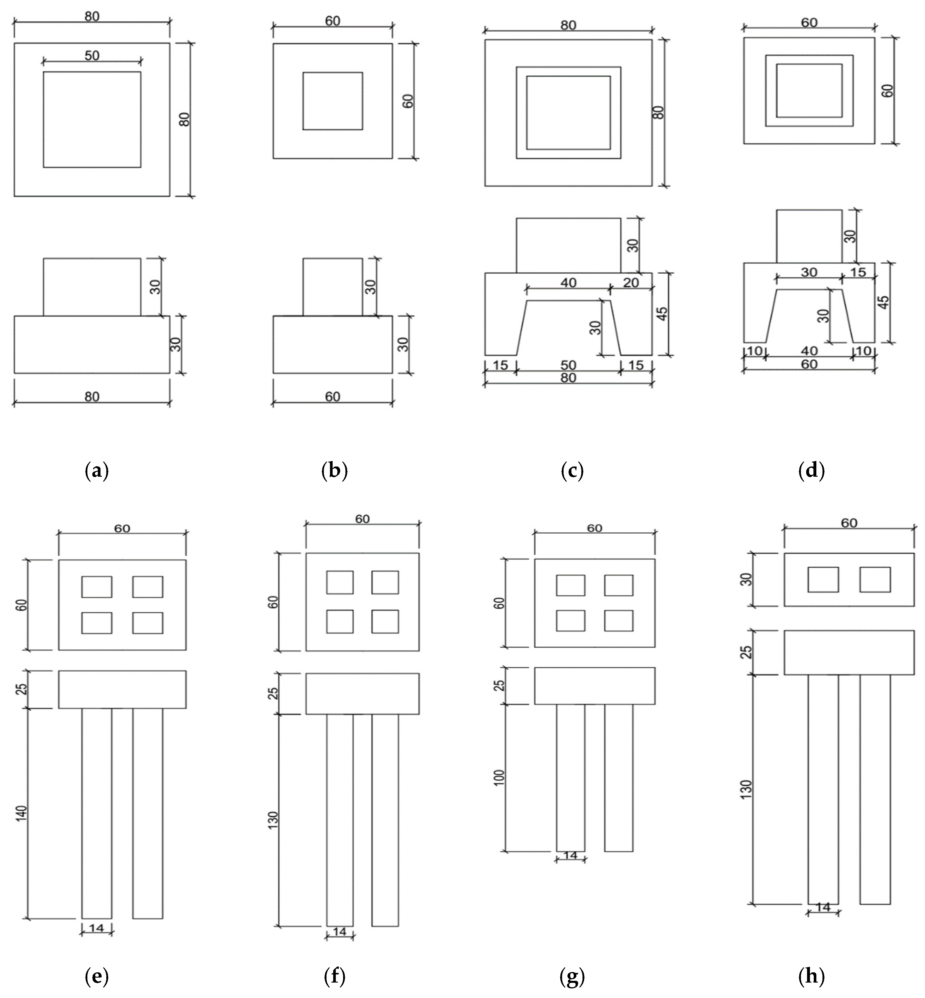
2.1. Foundation Models and Test Method

The model test considered three types of widely used bridge foundations: spread, caisson, and grouped pile foundations. In total, eight test models were prepared by considering different foundation sizes, namely large and small spread foundations (S1 and S2), large and small caisson foundations (C1 and C2), and four grouped pile foundations with different pile lengths and pile numbers (P1–P4), as illustrated in Figure 2 and Figure 3.
All the models were cast in situ using self-mixed concrete. Each model foundation to be tested was placed within the sand tank individually.
The tests using the TRM were performed using a 2 kg steel bar that impacted the top of the foundation (Figure 4a), and both force signals and velocity responses were recorded. Four velocity sensors were installed along the four edges at the foundation top (Figure 3c), and the average velocities obtained from the four sensors were used to calculate the dynamic stiffness.
The SLTs were performed using the laboratory reaction frame and a 10 t manual jack. The tests followed the slow maintenance loading method [36]. The values of vertical loading and vertical displacement were recorded using pressure and displacement sensors (Figure 4b). Based on the load–settlement curve (Ps curve) of the test, the static stiffness and bearing capacity were obtained.

2.2. Soil Parameter Test
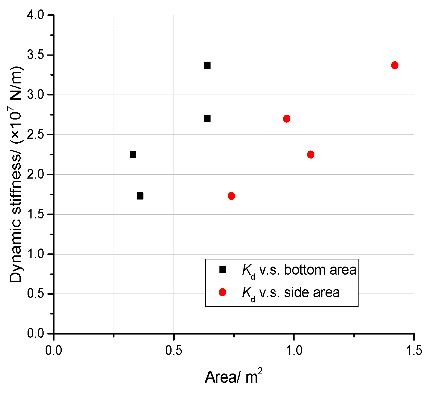
The dimensions of the sand tank were 2.3 m × 1.7 m × 1.5 m (Figure 5). The main soil parameters were tested in detail. The mass density was measured by the cutting ring method. The measured moisture rate is 1.54%, the mass of the cutting ring is 38 g, the total mass of the cutting ring and wet soil is 131.08 g. As the volume of the cutting ring is 60 cm2, the natural density and dry density are 1.551 and 1.548 g/cm3, respectively. The void ratio is 0.724.
Figure 6 illustrates the grain size diagram. The test sample can be determined as the medium sand. By the direct shear method, the cohesion and the angle of internal friction can be determined as: c = 2.4714 kPa and φ = 12.20°. The sand tank was filled with the sand and the filling sand was levelled every 40 cm height. According to different models, the model was preloaded with 1 ton weight pressure in advance. After the settlement remains stable for 24 h, other tests can be carried out.

3. TRM Test

3.1. Foundation Fully Buried in the Soil

The dynamic stiffness can be calculated as a function of the frequency using Equation (1). The TRM tests were repeated five times for each foundation model, and the average values of Kd(f) are illustrated in Figure 7. Owing to the limited impact mass, the Kd(f) values below 10 Hz were small, values between 10 and 50 Hz increased slowly with the frequency, and values increased sharply for frequencies above 50 Hz for most model foundations. Table 1 lists the Kd values of all foundation models for frequencies in the range of 10–50 Hz.
For the spread foundation, the Kd of model S1 can be calculated as approximately 1.56–1.71 times that of S2 between 10 and 50 Hz. The ratio of the bottom area of model S1 to that of S2 is 1.78, whereas the ratio of the side areas of these two models is 1.33. For the caisson foundation, the Kd of model C1 can be calculated as approximately 1.5–1.6 times that of C2 between 10 and 50 Hz. The ratio of the bottom area of model C1 to that of C2 is 1.94, whereas the ratio of the side areas of these two models is 1.33. That is, the ratio of the Kd values of the two models is between the values of the ratios of the side and bottom areas, which is in good agreement with the actual constraint state and bearing capacity. Figure 8 illustrates the variations in the dynamic stiffnesses of the spread and caisson foundations with the side and bottom areas. The values of Kd increase with both the side and bottom areas, thus indicating that the dynamic stiffness value can reflect the bearing capacity condition.
For the grouped pile foundation, as all the piles were friction piles, their bearing capacities were mainly attributed to the friction areas. Figure 9 illustrates the relationship between the dynamic stiffnesses and total side areas of all the piles. The trends of the curves are similar between 10 and 50 Hz. The dynamic stiffness thus increases with the total side area of the pile and exhibits an exponential growth rather than a linear growth.

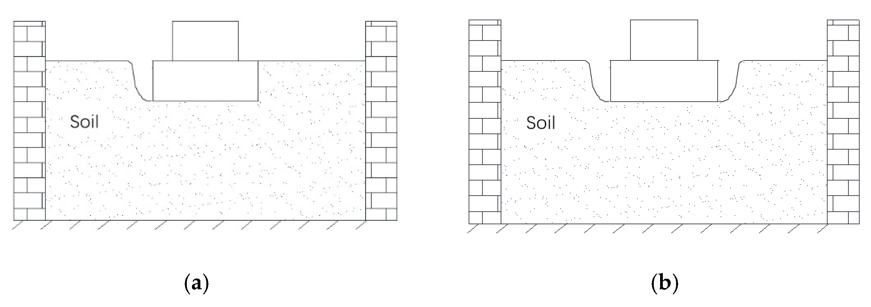
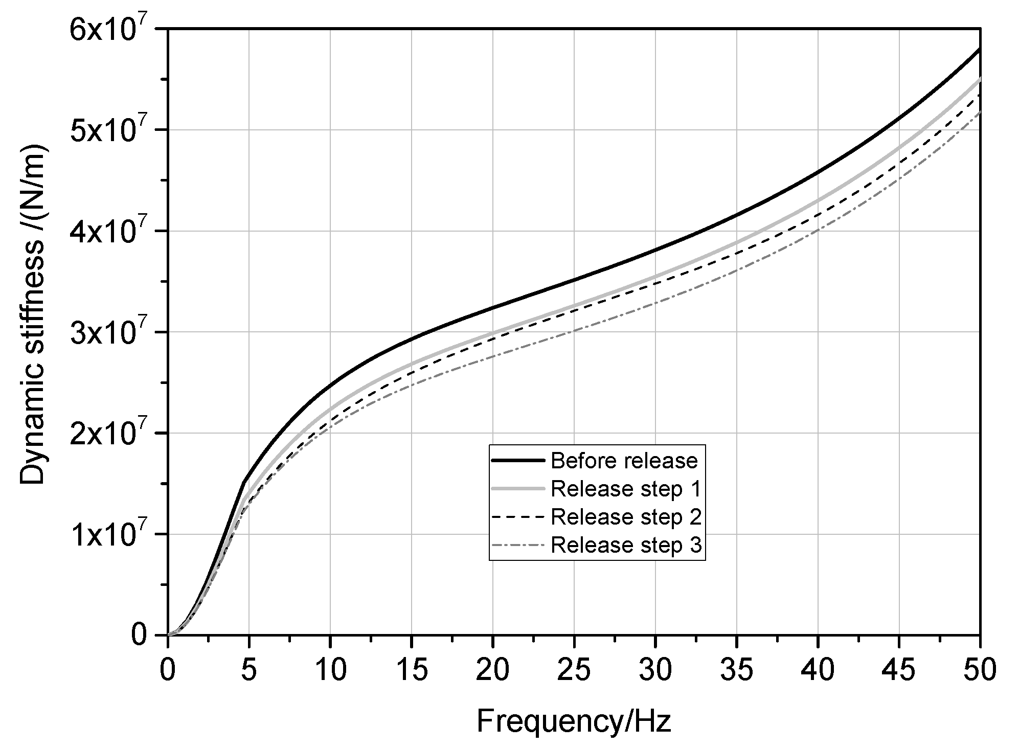
3.2. Change Foundation Constraint State

The constraint state of the foundation, including the supporting stiffness on the foundation bottom and side friction, is one of the significant factors affecting its bearing capacity. The ability of the dynamic stiffness to reflect the changes in the restraint state is directly related to whether the dynamic stiffness can effectively help evaluate the foundation state. Therefore, in the scale model tests, the following two aspects are mainly analysed: first, the Kd values of foundations that are fully buried in the soil and directly located on the ground are compared; second, the Kd values of foundations with different buried depths are analysed.
Figure 10 illustrates the three types of foundations directly located on the ground and fully buried in the soil. The impact on the foundation surface as well as both force and velocity responses are recorded. Then, the dynamic stiffnesses are obtained using Equation (1). Figure 11 shows a comparison of the Kd(f) values of different foundation models located on the ground and fully buried in the soil. Below 100 Hz, the values of Kd(f) increase logarithmically with frequency f when the foundation models are located on the ground, whereas these increments are exponential with frequency f when the foundation models are fully buried in the soil. As the ground can provide an extremely strong and stiff support to a foundation, in the low-frequency range (<50 Hz), the values of Kd(f) are obviously larger when the foundation models are located on the ground. Therefore, the Kd(f) in the low-frequency range can reflect the vertical support stiffness to some extent.
The above tests are extreme cases when the foundation models are located on the ground. However, it is almost impossible in practical engineering applications to obtain such large values of the vertical support stiffness. Therefore, in the following tests, the soil constraint state of the foundation model is changed, and the law of the dynamic stiffness change is analysed when the contact area between the soil and foundation model decreases. The tests were performed only on models S1, P1, and P3 as typical foundations of each type.
For the spread foundation model S1, changes to the soil constraint states are analysed in three steps, as illustrated in Figure 12. In these three steps, the foundation model was always in the loaded state. Figure 13 shows the Kd(f) value changes with the soil constraint states. With the release of the soil constraint around the foundation, the soil–structure contact area decreases, and the Kd(f) value decreases accordingly.
As illustrated in Figure 14, changes in the pile buried depths h = 1.35 m, 1.15 m, 0.95 m, 0.7 m, and 0.05 m for the grouped pile foundation model P1 (H = 1.4 m), and h = 0.7 m, 0.4 m, and 0.1 m for model P3 (H = 1.0 m) were computed.
Figure 15 and Figure 16 illustrate the dynamic stiffness changes with the pile buried depths for models P1 and P3. With the decrease in the pile buried depths, the Kd values decrease. The Kd values exhibit a linear relationship with h, and the correlation coefficients of linear fitting for the 10 Hz frequency are 0.989 and 0.953 for P1 and P3, respectively.

4. SLT Results

The test results in Section 3.2 show that there is an obvious relationship between the dynamic stiffness and foundation constraint state. To quantitatively analyse the relationship between the foundation capacity and dynamic stiffness, SLTs were performed. Figure 17 illustrates the load–settlement curves (Ps curve) for the three types of foundations. For each foundation type, the absolute value of the slope is smaller for foundation models with larger sizes and relatively greater design capacities. That is, under the same vertical load, the foundation models with larger sizes have stronger resistances to vertical settlement or higher static stiffnesses. In addition, the loading values corresponding to the inflection points in the Ps curves of the spread and caisson foundations are higher than those of the grouped pile foundations. This indicates that the spread and caisson foundations have larger allowable bearing capacities, which is consistent with the design size of the model foundation and the actual situation.
During the SLT, the Ps curve exhibits a linear relationship at the initial loading stage. Figure 18 illustrates the initial loading stages and corresponding linear fitting results of the three types of foundations. The correlation coefficients are greater than 0.99 for the spread and caisson foundations and exceed 0.97 for the grouped pile foundations. Then, the fitting results were used to calculate the static stiffnesses.
Figure 19 illustrates the relationship between the dynamic and static stiffnesses of the three types of foundations. For the spread foundations, the static stiffness ratio of models S1 to S2 is 1.51, whereas the average dynamic stiffness ratio of models S1 to S2 is 1.64. For the caisson foundations, the static stiffness ratio of models C1 to C2 is 1.73, whereas the average dynamic stiffness ratio of models C1 to C2 is 1.55. The two groups of ratios are close to each other. For the grouped pile foundations, the average dynamic stiffnesses exhibit a logarithmic growth trend with increase in the static stiffness, showing that there is a strong correlation between the dynamic and static stiffnesses. Generally, the bearing capacities of foundations can be controlled by deformation or strength under different loading conditions. When the capacity is controlled by the vertical deformation, the capacity can be described by the static stiffness value. That is, the dynamic stiffness is a sensitive index that can be used to evaluate the foundation capacity.

5. Conclusions

To evaluate the vertical capacity of bridge substructures using TRM and analyse the correlation between the dynamic and static stiffnesses by experimental method, in the present study a novel model test was performed in the laboratory, where both the TRM and SLT were used to assess three types of bridge foundations: spread, caisson, and grouped pile foundations. The dynamic stiffnesses were analysed when the foundations were first fully buried in the soils and then when the constraint states were changed. Subsequently, the static stiffnesses were calculated using the SLT results. Finally, the relationship between the dynamic and static stiffnesses was analysed. The conclusions can be drawn from the experimental results:
  • The index of dynamic stiffness can adequately reflect the foundation bearing capacity. Further, it can recognise changes in the foundation constraint state, such as vertical supporting stiffness on the foundation bottom, side, or bottom contact area, pile length, and pile buried.
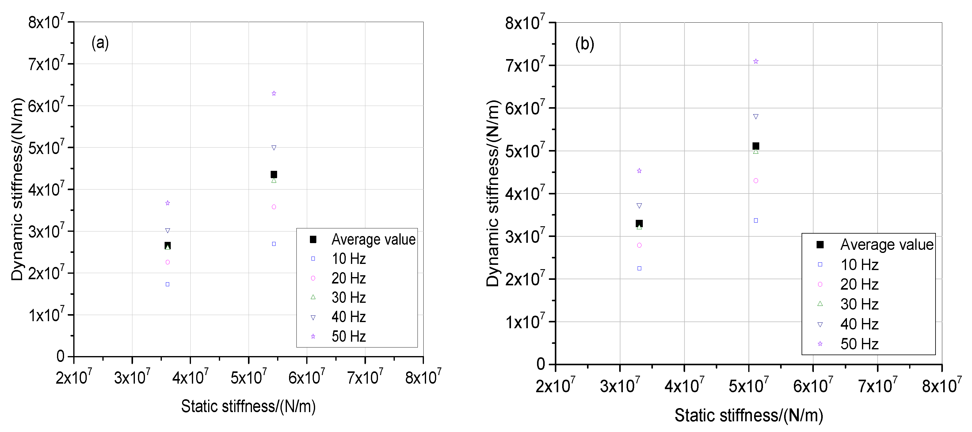
  • There is an obvious correlation between the dynamic and static stiffnesses.
  • The TRM can be employed to evaluate different foundation types, including spread, caisson, and grouped pile foundations.

Author Contributions

Conceptualization, J.L.; methodology, J.L. and M.M.; formal analysis, J.L. and M.M.; investigation, J.L. and M.M.; writing—original draft preparation, M.M.; writing—review and editing, J.L.; funding acquisition, J.L. All authors have read and agreed to the published version of the manuscript.

Funding

This research was funded by the Science and Technology Innovation Project of the National Energy Group (No. SHGF-14-50).

Institutional Review Board Statement

Not applicable.

Informed Consent Statement

Not applicable.

Data Availability Statement

Not applicable.

Conflicts of Interest

The author declared that there is no conflict of interest to this work.

References

  1. Carnevale, M.; Collina, A.; Peirlinck, T. A feasibility study of the drive-by method for damage detection in railway bridges. Appl. Sci. 2019, 9, 160. [Google Scholar] [CrossRef] [Green Version]
  2. Mousavi, M.; Holloway, D.; Olivier, J.C. Using a moving load to simultaneously detect location and severity of damage in a simply supported beam. J. Vib. Control. 2019, 25, 2108–2123. [Google Scholar] [CrossRef]
  3. Dai, G.L.; Gong, W.M.; Zhao, X.L.; Zhou, X. Static Testing of Pile-Base Post-Grouting Piles of the Suramadu Bridge. Geotech. Test. J. 2011, 34, 34–49. [Google Scholar]
  4. Chandrasekaran, S.; Banerjee, S. Retrofit optimization for resilience enhancement of bridges under multihazard scenario. J. Struct. Eng. 2016, 142, C4015012. [Google Scholar] [CrossRef]
  5. Jung, W.; Yune, C.; Lee, I. Evaluation of Performance Simulation for Bridge Substructure Due to Types of Scour. J. Korean Geoenviron. Soc. 2013, 14, 5–11. [Google Scholar]
  6. Zhang, X.Y.; Chen, X.C.; Wang, Y.; Ding, M.; Lu, J.; Ma, H. Quasi-static test of the precast-concrete pile foundation for railway bridge construction. Adv. Concr. Constr. 2020, 10, 49–59. [Google Scholar]
  7. Prendergast, L.J.; Gavin, K. A review of bridge scour monitoring techniques. Int. J. Rock Mech. Min. Sci. 2014, 6, 138–149. [Google Scholar] [CrossRef]
  8. Makris, N.; Badoni, D.; Delis, E.; Gazetas, G. Prediction of observed bridge response with soil-pile-structure interaction. J. Struct. Eng. 1994, 120, 2992–3011. [Google Scholar] [CrossRef]
  9. Guin, J.; Banerjee, P.K. Coupled soil-pile-structure interaction analysis under seismic excitation. J. Struct. Eng. 1998, 124, 434–444. [Google Scholar] [CrossRef]
  10. Dutta, S.C.; Roy, R. A critical review on idealization and modeling for interaction among soil–foundation–structure system. Comput. Struct. 2002, 80, 1579–1594. [Google Scholar] [CrossRef]
  11. Avent, R.R.; Alawady, M.; Guthrie, L. Underwater bridge deterioration and the impact of bridge inspection in Mississippi. Transp. Res. Rec. J. Transp. Res. Board 1997, 1597, 52–60. [Google Scholar] [CrossRef]
  12. Avent, R.R.; Alawady, M. Bridge scour and substructure deterioration: Case study. J. Bridge Eng. 2005, 10, 247–254. [Google Scholar] [CrossRef]
  13. Zhan, J.W.; Xia, H.; Yao, J.B. Damage evaluation of bridge foundations considering subsoil properties. In Environmental Vibrations: Prediction, Monitoring, Mitigation and Evaluation (ISEV 2005); Taylor & Francis: Milton Park, UK, 2005; pp. 271–277. [Google Scholar]
  14. Kien, P.H. Application of impact vibration test method for bridge substructure evaluation. MATEC Web Conf. 2017, 138, 02017. [Google Scholar] [CrossRef] [Green Version]
  15. Lombaert, G.; Degrande, G.; Kogut, J.; Francois, S. The experimental validation of a numerical model for the prediction of railway induced vibrations. J. Sound Vib. 2006, 297, 512–535. [Google Scholar] [CrossRef]
  16. Ma, M.; Li, M.H.; Qu, X.Y.; Zhang, H.G. Effect of passing metro trains on uncertainty of vibration source intensity: Monitoring tests. Measurement 2022, 193, 110992. [Google Scholar] [CrossRef]
  17. Sanchez-Quesada, J.C.; Moliner, E.; Romero, A.; Galvin, P.; Martinez-Rodrigo, M.D. Ballasted track interaction effects in railway bridges with simply-supported spans composed by adjacent twin single-track decks. Eng. Struct. 2021, 247, 113062. [Google Scholar] [CrossRef]
  18. Xu, L.H.; Ma, M. Dynamic response of the multilayered half-space medium due to the spatially periodic harmonic moving load. Soil Dyn. Earthq. Eng. 2022, 157, 107246. [Google Scholar] [CrossRef]
  19. Olson, L.D. Dynamic Bridge Substructure Evaluation and Monitoring; FHWA-RD-03-089; US Department of Transportation Federal Highway Administration: Washington, DC, USA, 2005.
  20. Fellenius, B.H.; Harris, D.E.; Anderson, D.G. Static loading test on a 45 m long pipe pile in Sandpoint, Idaho. Can. Geotech. J. 2004, 41, 613–628. [Google Scholar] [CrossRef]
  21. Budi, G.S.; Kosasi, M.; Wijaya, D.H. Bearing capacity of pile foundations embedded in clays and sands layer predicted using PDA test and static load test. Procedia Eng. 2015, 125, 406–410. [Google Scholar] [CrossRef]
  22. Muszynski, Z.; Rybak, J. Application of geodetic measuring methods for reliable evaluation of static load test results of foundation piles. Remote Sens. 2021, 13, 3082. [Google Scholar] [CrossRef]
  23. Wang, Z.Y.; Zhang, N.; Cai, G.J.; Li, Q.; Wang, J. Assessment of CPTU and static load test methods for predicting ultimate bearing capacity of pile. Mar. Georesour. Geotechnol. 2016, 35, 738–745. [Google Scholar] [CrossRef]
  24. Liu, S.W.; Zhang, S.M.; Zhang, J. Analysis on modification of the measured results of test pile due to the influence of reaction piles in static loading test. Geotech. Test. J. 2016, 39, 712–720. [Google Scholar]
  25. Baca, M.; Brzakala, W.; Rybak, J. Bi-directional static load tests of pile models. Appl. Sci. 2020, 10, 5492. [Google Scholar] [CrossRef]
  26. Liang, R.Y. New wave equation technique for high strain impact testing of driven piles. Geotech. Test. J. 2003, 26, 111–117. [Google Scholar]
  27. Svinkin, M.R. High-strain dynamic pile testing—Problems and pitfalls. J. Perform. Constr. Facil. 2010, 24, 99. [Google Scholar] [CrossRef]
  28. Liang, L.; Beim, J. Effect of soil resistance on the low strain mobility response of piles using impulse transient response method. In Proceedings of the 8th International Conference on the Application of Stress Wave Theory to Piles, Lisbon, Portugal, 8–10 September 2008. [Google Scholar]
  29. Davis, A.G. The nondestructive impulse response test in North America:1985–2021. NDTE Int. 2003, 36, 185–193. [Google Scholar] [CrossRef]
  30. Geotechnical Control Office Foundation Design and Construction; GEO Publication: Hong Kong, China, 2006.
  31. Lo, K.F.; Ni, S.H.; Huang, Y.H. Non-destructive test for pile beneath bridge in the time, frequency, and time-frequency domains using transient loading. Nonlinear Dyn. 2010, 62, 349–360. [Google Scholar] [CrossRef]
  32. Liu, J.L.; Ma, M. Analysis of the dynamic stiffness and bearing capacity for pile foundations. Vibroeng. Procedia 2015, 5, 134–139. [Google Scholar]
  33. Ma, M.; Liu, J.; Ke, Z.; Gao, Y. Bearing capacity estimation of bridge piles using the impulse transient response method. Shock. Vib. 2016, 2016, 4187026. [Google Scholar] [CrossRef] [Green Version]
  34. Chu, J.H.; Ma, M.; Liu, J.B. Analysis of dynamic stiffness of bridge cap-pile system. Shock. Vib. 2018, 2018, 7645726. [Google Scholar] [CrossRef] [Green Version]
  35. Liu, J.L.; Ma, M. A full-scale experimental study of the vertical dynamic and static behavior of the pier-cap-piles system. Adv. Civ. Eng. 2020, 2020, 9430248. [Google Scholar] [CrossRef]
  36. Shi, L.; Qi, C. In-situ experimental investigation on pullout performances and horizontal bearing properties of bored piles. Springer Ser. Geomech. Geoengin. 2018, 204379, 234–247. [Google Scholar]
Figure 1. Theoretical mobility response spectrum tested using the TRM.
Applsci 12 04951 g001
Figure 2. Dimensions of the eight fabricated test models (unit: cm). (a) Model S1; (b) model S2; (c) model C1; (d) model C2; (e) model P1; (f) model P2; (g) model P3; (h) model P4.
Applsci 12 04951 g002
Figure 3. Pictures of the various model foundations: (a) grouped pile foundation models; (b) spread foundation models; (c) caisson foundation model and its sensor locations.
Applsci 12 04951 g003
Figure 4. Test equipment: (a) impact steel bar; (b) equipment and sensors for the SLT.
Applsci 12 04951 g004
Figure 5. Cross-sectional views of the sand tank configurations in the laboratory: (a) spread foundation; (b) caisson foundation; (c) grouped pile foundation.
Applsci 12 04951 g005
Figure 6. Grain size diagram.
Applsci 12 04951 g006
Figure 7. Dynamic stiffnesses of the eight foundation models: (a) spread foundations; (b) caisson foundations; and (c) grouped pile foundations.
Applsci 12 04951 g007
Figure 8. Dynamic stiffness value variations in the spread and caisson foundations with side and bottom areas.
Applsci 12 04951 g008
Figure 9. Relationships between the dynamic stiffnesses and total side areas of the ground piles.
Applsci 12 04951 g009
Figure 10. Foundation models located on the ground and fully buried in the soil: (a) spread foundation; (b) caisson foundation; (c) grouped pile foundation.
Applsci 12 04951 g010
Figure 11. Comparisons of the Kd(f) values of different foundation models located on the ground and fully buried in the soil: (a) model S1; (b) model S2; (c) model C1; (d) model C2; and (e) model P3.
Applsci 12 04951 g011aApplsci 12 04951 g011b
Figure 12. Changes to the soil constraint state on model S1: (a) soil constraint released on one side; (b) soil constraint released on two sides; and (c) soil constraints released on two sides and a corner.
Applsci 12 04951 g012aApplsci 12 04951 g012b
Figure 13. Dynamic stiffness changes with soil constraint states for model S1.
Applsci 12 04951 g013
Figure 14. Changes to the pile buried depths in models P1 and P3.
Applsci 12 04951 g014
Figure 15. Dynamic stiffness changes for various pile buried depths for model P1: (a) Kd(f) function; and (b) Kd values at 10, 20, 30, 40, and 50 Hz.
Applsci 12 04951 g015
Figure 16. Dynamic stiffness changes for various pile buried depths for model P3: (a) Kd(f) function; and (b) Kd values at 10, 20, 30, 40, and 50 Hz.
Applsci 12 04951 g016
Figure 17. SLT Ps curves of the (a) spread; (b) caisson; and (c) grouped pile foundations.
Applsci 12 04951 g017
Figure 18. Linear fittings of the static loading test Ps curves during the initial loading stage: (a) spread foundation; (b) caisson foundation; and (c) grouped pile foundation.
Applsci 12 04951 g018aApplsci 12 04951 g018b
Figure 19. Relationship between the dynamic and static stiffnesses: (a) spread foundation; (b) caisson foundation; and (c) grouped pile foundation.
Applsci 12 04951 g019aApplsci 12 04951 g019b
Table 1. Kd values of all foundation models for frequencies in the range of 10–50 Hz.
ModelDynamic Stiffness/(×107 N/m)
10 Hz20 Hz30 Hz40 Hz50 Hz
Model S12.703.584.205.016.29
Model S21.732.262.603.033.67
Model C13.374.304.975.827.09
Model C22.252.793.203.734.53
Model P19.6212.1013.0513.6514.60
Model P27.889.289.8810.4211.06
Model P33.163.904.405.045.96
Model P42.382.873.093.273.50
Publisher’s Note: MDPI stays neutral with regard to jurisdictional claims in published maps and institutional affiliations.

