Abstract
In downhole drilling systems, self-excited torsional vibrations caused by the bit-rock interactions can affect the drilling process and lead to the premature failure of components. Especially self-excited oscillations of higher-order modes lead to critical dynamic loads. The slim drill string design and the naturally limited drilled borehole diameter limit the installation space, power supply and lead to numerous potentially critical self-excited torsional modes. Consequently, small and robust passive damping concepts are required. The variety of possible downhole boundary conditions and potential damper designs necessitates analytical solutions for effective damper design and optimization. In this paper, two nonlinear passive damper concepts are investigated regarding design and effectiveness to reduce self-excited high-frequency torsional oscillations in drill string dynamics. Based on a finite element model of a drill string, a suitable minimal model based on the identified critical mode is generated and solved analytically using the Multiple Scales Lindstedt-Poincaré (MSLP) method. The advantages of MSLP compared to conventional MS methods are shown for this example. On the basis of the analytical solution, parameter influences are determined, and design equations are derived. The analytical results are transferred to self-excited drill string vibrations and discussed using time domain simulations of the drill string model.
1. Introduction
In deep drilling applications, unwanted vibrations can reduce reliability, lead to premature failures of components, reduce the drilling efficiency and increase nonproductive time. Around one-third of all failures in drilling applications are related to vibrations [1,2]. The occurring vibrations are divided into axial, lateral and torsional vibrations according to their operating direction. Since the late 1960s, torsional vibrations have been the research focus [3,4]. Torsional vibrations are divided into low- and high-frequency vibrations. Low-frequency vibrations like stick/slip correspond to the first torsional mode of the drilling system, with frequencies less than 1 Hz. These self-excited vibrations are distinguished according to their origins in bit and string-induced vibrations. Bit-induced vibrations originate from the bit-rock cutting process, while string-induced vibrations are caused by the contact between drilling tools and formation [5]. The bit rock interaction during drilling is a complex process with many uncertainties [6], which can be considered, in various ways, e.g., with hybrid uncertainties [7]. It has been shown that, for the torsional dynamic of the drill string, the energy input can be modeled using a nonlinear torque characteristic at the bit [8]. Due to improved and new measuring tools, high-frequency oscillations have been identified as the cause of numerous drill string failures and have been intensively investigated over the last years with studies [9,10], simulations [8,11] and experiments [12,13]. Especially drilling in hard and dense formations leads to high-frequency torsional oscillations (HFTO) with frequencies between 50 Hz and 500 Hz [14,15]. By assuming a resistance characteristic at the bit (torque characteristic) that decreases with the angular speed (revolutions per minute RPM) (Figure 1), a predictive criterion based on linearization at the operation point (
is derived [8], wherein represents the modal damping, the natural angular frequency and the deflection of the mass normalized eigenvector of mode k.
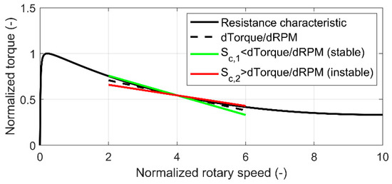
Figure 1.
Nonlinear torque characteristic at the bit cf. [8].
Additionally, a maximum amplitude at the bit () that depends on the revolutions per minute (RPM) in the operating point
is derived in [16] and agrees with the observations in [14] that no backward rotation occurs at the bit. This maximum amplitude is valid when one HFTO mode dominates the dynamic of the entire drill string [17,18]. In [17], the interaction between stick/slip and HFTO is observed and [19] analyzed in detail. Using the information about stick/slip, HFTO and the torque characteristic (Figure 1) stability maps are derived [19] and new strategies to reduce vibrations by adjusting operational parameters like the drilling velocity (RPM) and the downhole force on the bit (in drilling industry: weight on bit (WOB)) are shown [5]. As neither the parameters nor the design of the drill string can be changed arbitrarily, new downhole tools must be developed to reduce critical vibrations. An isolator tool based on the principle of mechanical low-pass filtering is analyzed in testing, simulation and operation [13] and reduces the amplitude in specific areas of the BHA. As the isolator does not mitigate the critical vibration along the entire drill string, further mitigation strategies are necessary. Increasing the damping of a system is a common approach to reduce self-excited vibration [20,21]. In [22], the effects of various friction dampers on the stability of critical HFTO modes are analyzed. The derived analytical results show the importance of damper placement regarding the multiple instable modes and multiple damper positions within the BHA.
Due to the large number of variable parameters such as the critical mode (frequency and mode shape), the position of the damper and the design of the damper, analytical solutions with regard to the effective damping range of the damper are necessary for an effective design and optimization of dampers in drill string dynamics. Therefore, as in [22], analytical and semi-analytical solutions regarding the effective damping range of the dampers must be determined. For nonlinear dampers, various methods to approximate nonlinearities exist. The harmonic balance method [23,24,25] is one possibility to approximate nonlinear parts of a differential equation that has been used for drill string dynamic [22]. Especially for tuned systems like nonlinear tuned mass dampers, methods like the Multiple Scales (MS) [26] or Lindstedt-Poincaré (LP) [27] are suitable approximation options. Multiple Scales Lindstedt-Poincaré (MSLP) is the rather new combination of MS and LP to solve nonlinear systems [28].
In the following, the MSLP method is used to determine suitable analytical solutions for various nonlinear tuned damper concepts to reduce high-frequency torsional vibrations within the drill string. First, a suitable finite element (FE) model of a drill string is developed and reduced to one modal degree of freedom representing a critical torsional mode. This minimal model is extended by two tuned nonlinear damper concepts. Similar to a tuned mass damper, the basic structure of both nonlinear dampers consists of an inertia mass that is connected by a linear spring and linear damper to the structure. One nonlinear damper has an additional cubic nonlinear stiffness, and the other, a cubic nonlinear stiffness and a friction contact. Second, the resulting nonlinear models are solved using MSLP. It is shown that in this specific case MSLP is more accurate than other methods, like the MS method. Third, the parameter influences are determined, and the analytical solutions are transferred to a self-excited drill string vibration to realize a robust and optimized design. Finally, the analytical results are compared with time domain simulations of self-excited drill string vibrations using a reduced FE drill string model. Furthermore, influences and design specifications for drill string vibrations are discussed.
2. Modeling
2.1. Extended Drill String Model
To investigate the effect of the nonlinear dampers on the torsional dynamics of the drill string, a generic drill string model (Figure 2) was constructed using beam elements. The resulting linear equation of motion
consists of the mass , damping and stiffness matrix, an external force vector and the angular deviations from the operating point for a static twist and constant rotary speed.
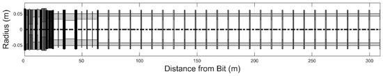
Figure 2.
Generic model of a bottom hole assembly (Baker Hughes).
The mass and stiffness matrix are determined from the design of the generic bottom hole assembly (BHA) using Young’s modulus, density and geometry, while the damping matrix is unknown. Previous studies show that, in many cases, a critical mode dominates the system behavior [17,18]. Therefore, the damping matrix can be determined by the modal damping ratio of the modes. Using the predictive criterion derived in [8] and determining the value, the BHA can be reduced to a single modal degree of freedom representing the critical high frequency mode. This modal reduction of the torsional dynamic of a drill string is despite its complexity suitable, because when HFTO occur, mostly one critical mode dominates the entire torsional system dynamic of the BHA. In addition, the large but slim design of the drill string with little available installation space leads to low reactive effects of dampers on the torsional dynamics of the drill string. In [8,16,19], a similar reduction method was used to characterize downhole vibrations and in [5,19,22] ‘it is used to investigate vibration reduction strategies.
2.2. Minimal Model of a Drill String and Damper
Assuming that the reactive effect of the damper on the mode is negligible due to the limited installation space in deep drilling and the assumption that no other modes near the considered mode or higher harmonics are excited by the nonlinear forces [22], a modal single degree of freedom (sdof) was derived. The modal reduction of the extended drill string model yields to
consisting of the angular natural frequency , the modal damping , the modal deviation of the considered mode and an external torque acting at the -th node (position) with a mass normalized modal amplitude of the -th mode at the -th node. By adding the degree of freedom representing the considered damper, the minimal model yields
consisting of the physical degree of freedom of the damper , the inertia of the damper , the linear stiffness and linear damper connecting the damper and the structure at the -th node. The nonlinear torque is
with a cubic stiffness for the cubic nonlinearity and
for the cubic nonlinearity and the additional frictional contact consisting of a normal force , friction radius and coefficient of friction .
2.3. Adaption and Simplification of the Minimal Model
With the assumption that the additional damper does not influence the movement of the drill string itself, but only the modal amplitude via the energy balance, the vibration of the structure is assumed to be harmonic,
similar to the harmonic balance. The resulting equation of motion of the damper
represents a sdof-model. By introducing the difference coordinates and their derivations, the amplitude and phase of the system were directly taken into account in the results due to the considered relative motion. The equation of motion for the damper with cubic nonlinearity is
and with cubic nonlinearity and a friction contact is
3. Applying Multiple Scales Lindstedt-Poincarè
3.1. Multiple Scales Lindstedt-Poincarè
A quite new technique for analyzing nonlinear systems is the Multiple Scales Lindstedt-Poincaré method was first introduced by Pakdemirli in 2009 in [28]. As the method’s name already shows, it is a combination of both the Multiple Scales (MS) [26] and the Lindstedt-Poincaré (LP) [26,27] method. A small parameter is introduced to perform the MSLP. The modal natural angular frequency of the structure is now expressed as and, to simplify following equations, all parameters concerning the friction damper are expressed through the summarizing variable .
In analogy to the LP method, a new time variable is introduced and further divided according to the MS method in
while the dividing of the replacement variable stays the same with
and is now only dependent on . The introduced frequency now has the structure
and slightly differs from those introduced in the LP method. The next step is inserting these expressions in the nonlinear differential equation of motion and separating for the orders of similar to LP, although, in contrast to LP is replaced. The secular terms in the higher order equations have two unspecified expressions, one being the time derivative of the complex amplitude out of the MS, the other being the frequency expression out of LP. Setting these terms follows a simple rule: is set to zero, giving an expression for unless it is a complex expression; then, is set to zero, giving an expression for .
The main goal is to make sure no complex expressions occur for the frequency . The combination of the derivatives of the complex amplitude follows the same steps as those for the MS. The same applies to the combining of the frequencies regarding LP.
3.2. Applying MSLP on the Damper with Cubic Nonlinearity
In the following, the MSLP method is applied to the drill string model (Equation (10)) to find the analytical results to determine the steady-state amplitude. A small parameter is introduced, and Equation (10) is normalized regarding the inertia
with , and . Introducing MSLP coordinates leads to
Using the detuning parameter , can be written as . Now, Equation (5) becomes
and simplifies the agreement in analyzing only up to to
A separation regarding the order leads to
with representing the time derivative. Equation (8) solves
with being the complex amplitude with its complex conjugates and denote the complex conjugate of the previous expression. The secular terms of the equation of are
and the same for the complex conjugate expression. For secular terms in MSLP, is set to zero, giving
Now, Equation (20) results in the particular solution
recalling again that the homogenous solution is already compensated by the result Equation (10) of Equation (8). The right-hand side of Equation (7) can be written as
using the detuning parameter to express . By that, the secular terms of are
Setting equal to zero leads to a complex expression for , as described above in this case, is set to zero, leading to
Using the Nayfehs method of recombination [27]:
the time derivative of the complex amplitude is
and introducing can rearrange the equation after a little manipulation
where a split into real and imaginary parts conducted for the steady state
By using mathematical identities:
is obtained and yields the frequency-response curve.
with
Without the frequency-response curve is
The solution of the equation of motion is obtained by using the solutions of the differential equations of and
3.3. Including Friction in MSLP
Including friction damping in the analysis creates the needs for approaching the sign function that changes the sign regarding the relative angular velocity, which characterizes the friction damping, by, e.g., polynomial expressions. Many ways of this are shown in the literature—for example, by Nayfeh in [26]. One way is to use a Fourier series to approximate the friction term .
Regarding the analysis, only multiples of the angular natural frequency are considered so that the expression can be simplified using only . The term
with is of interest for the secular terms. Introducing a new variable shortens Equation (40) to
This expression can now be placed in the term of the corresponding order of . This way of approximating the sign function also shows that considering analyzing higher orders of makes the analysis much more complicated, as then higher terms of the Fourier series are needed. The MSLP analysis of the combination of cubic stiffness and the friction contact (Equation (1)) lead to
with . By using and MSLP coordinates,
result in the same for and as the MSLP analysis for the damper with cubic stiffness (Equations (8) and (20)) and the friction damping terms affect solutions of and higher. Solving yields the secular terms
where is set to zero; otherwise, it would be complex, giving an expression for
The term resulting from the Fourier series must now be further analyzed. Therefore, it needs to be considered that
by which
can be separated into its real and imaginary parts, leading towards
so that the whole expression can be written as . This yields, similar to obtaining Equation (30) in the earlier MSLP, the combined derivative of the complex amplitude by
where splitting into real and imaginary parts results for the steady state in
In general, the frequency-response curve now turns out to be
with Equation (22) for or without
and
being the same as for the MSLP of the viscous damper. When using the solutions, including a friction damper, special attention should be paid to the stick and stick-slip areas of the friction damper. The friction damper can also be included in the analysis by using its equivalent viscous damping. However, the equivalent damping ratio
must be used after the MSLP coordinates are introduced with respect to the different characteristics of friction damping.
4. Advantages and Limitations of MSLP
4.1. Comparing MSLP and MS
Pakdemirli [28,29] has shown that there are minor differences between MS and MSLP solutions for normally excited damped systems with cubic nonlinearities. In this specific example with difference coordinates and an excitation that is dependent on the frequency, the MSLP method is more precise. However, not only the method can affect the accuracy of the solutions, the exponent of the small parameter also affects the feasibility of the analysis and, thus, the accuracy. Comparing the results obtained by MS using in the first power for the damping and excitation term, in the second power and MSLP with in the second power leads in the typical Multiple Scales analysis to
Using
and now analyzing only up to due to the very complex expressions for ; the function for the frequency-response curve is
It is important to recognize that, according to the power of in the equation describing the system, the expression for calculating the excitation frequency out of the detuning parameter and the angular natural frequency also changes according to for MS methods or for MSLP.
The differences in the obtained solutions are shown in Figure 3a,b in comparison to the results simulated in the time domain. MSLP results are accurate even for such large nonlinearities and excitations that subharmonic resonance occurs, MS solutions meanwhile show spurious peaks that are bend to much or in the wrong direction.
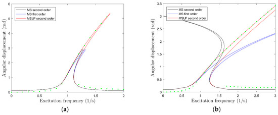
Figure 3.
Comparison of Multiple Scales Lindstedt-Poincaré (MSLP) and multiple scales (MS) analysis for with different order in (a) for small nonlinearities and (b) for strong nonlinearities . The green points represent the numerical obtained steady-state amplitudes.
In Figure 3a, the solutions of MS do not cover the whole excitation branch in contrast to the MSLP solution, which matches the point representing the numerically obtained solution very accurate. For the strong excitation in Figure 3b, MS solutions even show very differently bended curves than the numerical solution or MSLP. Furthermore, the MS solution for is bent backwards and, therefore, not just quantitatively but, also, qualitatively inaccurate. Due to the dependency of the excitation force on the excitation frequency in this case, the MSLP method is more suitable to approximate the equation of motion.
4.2. Limits of the Operating Range
The deviation of analytical and numerical solutions beyond the effective frequency range of the nonlinear damper, frequencies much higher or lower than the natural frequency of the damper (Figure 3b), are rather high. This is caused in the step of expressing the excitation frequency through the detuning parameter and then sorting the terms for only up to . Thereby, no attention is payed to the -characteristic of the excitation and it becomes the same as a normally excited system. This happens when the right-hand side of Equation (5) is rewritten by
with the use of the detuning parameter. When analyzing only up to this becomes
where , as being independent from the excitation, can simply be treated like another parameter among the others, and a “normal” excitation develops. However, as the damper has no significant effect outside the resonance area and, therefore, only the results for the resonance are of special interest; there is no such limiting factor, in this case. Furthermore, negative values for the nonlinearity parameter can cause problematic results in the case of weakening nonlinearities by bending the peaks of the frequency-response curve unphysically. Again, this is irrelevant for the considered cases.
4.3. Parameter Dependency of the Operating Range
For engineering purposes, it might be interesting to know the maximum amplitude of the system to set the parameters respective to the available space. The maximum difference amplitude can be calculated by looking at the square root of the frequency-response Equation (36) in question. Since the maximum point is the point where the expression containing the negative square root goes over into the expression with the positive square root, the maximum point is where both expressions are equal. This means that the square root is zero. Thereby
solves to
wherein only the positive square roots are being used. An additional friction element yields to a much larger expression for the maximum amplitude:
with
which is again obtained by analyzing the square root expression of the frequency-response equation in question. Using these techniques, a three-dimensional plot can be created, showing how the damping parameter and the coefficient of the nonlinearity affected the maximum amplitude for a given excitation.
As the point of the maximum amplitude is characterized by the square root in Equation (36) being zero, the frequency of the maximum amplitude can be described by
which, by the use of Equation (45), can be further simplified to
or
as an expression for the frequency shift of the viscous damper (see Figure 4a).
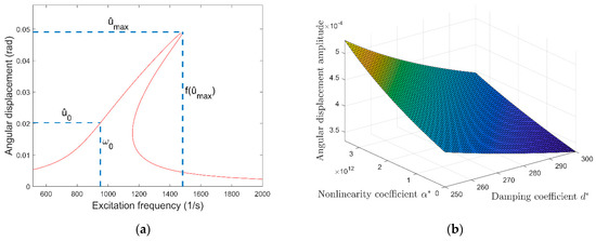
Figure 4.
Frequency-response curve with markings for the point of maximum amplitude and the point of the linear natural frequency (a) and the influence of the damping and nonlinearity coefficient on the maximum amplitude () (b).
Figure 4b shows again that a higher nonlinearity coefficient and a lower damping coefficient result in a higher maximum amplitude. According to the imagination, a higher nonlinearity coefficient leads to a higher frequency shift. However, an increase of the damping coefficient decreases this frequency shift as it decreases the maximum amplitude. Thereby, the combination of a very small maximum amplitude and a very large frequency shift can be a mutual contradiction.
5. Parameter Influences
5.1. Influence and Normalization of the Angular Natural Frequency
Changing the angular natural frequency has a huge effect on the frequency-response curve, because its center changes to another excitation frequency depending on . This has a large impact due to the characteristic of the right-hand side and its appearance in the argument of the cosine. Wanting to apply an obtained frequency-response curve to another excitation frequency requires not only a simple introduction of a frequency ratio but, also, an adjustment of the other parameters. Therefore, it is necessary to have a system that leads to the same resulting equation. In this angular frequency normalization, the units are used similar to Section 4. The units were considered during normalization; however, note that we omitted the unit label in the following for readability. Using Equation (4) with a new natural frequency according to the excitation frequency to achieve the same plot is . Inserting this and equalizing Equation (4) yields
with being some kind of response related to as discussed above. Therefore, , and . So and can give the same structure as the original differential equation and, therefore, the same frequency-response curve as for . This way of adapting the parameters can also be used when varying one of the others and wanting to achieve the same frequency-response curve.
Again, a consideration of a friction damper requires a deeper understanding of the method. The way as shown above would lead to , whereas the correct solution is , because the approach via Fourier series or equivalent damping ration includes an additional division by . This must be observed to get the same frequency-response curve.
5.2. Influence of the Normalized Parameters on the Dynamic Response of the Damper
Changing the system parameters affects the frequency-response curve and, thereby, the dynamic of the system in different ways. Changing the nonlinear stiffness of the cubic nonlinearity, for example, not only modifies the bending angle of the curve but, also, the length of the branches (Figure 5a).
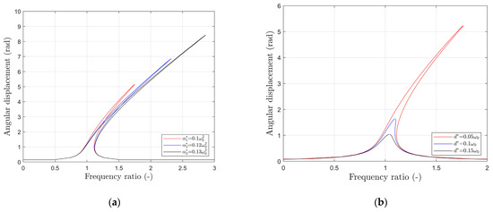
Figure 5.
Comparison of frequency-response curves when varying (a) the nonlinearity coefficient () and (b) the damping coefficient ().
Changing the damping ratio affects the length of the branch (Figure 5b). A higher damping ratio shortens the frequency-response curve and results in a smaller maximum amplitude.
The same applies when increasing the friction damping coefficient, here represented by (Figure 6a). It might be worth mentioning that a stronger friction force not only shortens the frequency-response curve but, also, slims down the foot of the branches around the natural frequency stronger than the viscous damping.
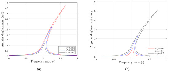
Figure 6.
Comparison of frequency-response curves when varying the (a) friction damping coefficient () and (b) excitation amplitude ().
Looking at the frequency-response curve in relation to the excitation, there are two parameters that can change. The one is the excitation frequency, and the other is the excitation amplitude. For the excitation amplitude, an increase results in an increase of the maximum amplitude; hence, the length of the curve (Figure 6b).
The variation of the inertia is more complex, because not only the parameters but the natural frequency of the system itself are changed (Figure 7).
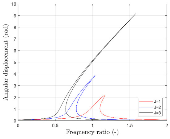
Figure 7.
Comparison of frequency-response curves when varying the inertia ().
6. Transfer to Self-Excited Drill String Vibrations
Section 4.1 shows that the analytical solutions derived using MSLP correspond well with the numerical simulations of the single degree of freedom system in Equation (9) (respectively, Equations (10) and (1)). In the following, the analytical solutions derived using MSLP are transferred to self-excited drill string vibrations using the equivalent damping ratio and discuss using time domain simulations based on Equation (5). Based on this, instructions for using the results in self-excited drill string systems are derived.
6.1. Energy Dissipation and Equivalent Damping
One possibility to transfer analytical solutions, based on the assumption of a constant harmonic amplitude of the underlying structure to self-excited structures, is the energy balance and the related equivalent damping ratio (cf. [22]). The dissipated energy of the damper can be calculated using the frequency-response curve (Equations (23) and (37)) and the equation of the damper motion (Equations (24) and (38)). In the case of a viscous damper with a cubic nonlinearity
is the dissipated energy. When analyzing a system containing viscous and friction damping with a cubic nonlinearity, the total dissipated energy consists of the dissipated energy of the viscous damper and the dissipated energy of the friction damper
over one period. As described in [22] and shown in Equation (1), the modal damping ratio is decisive for the stability and the resulting amplitude of the self-excited systems. Therefore, the total dissipated energy of the damper is converted by
in the equivalent modal damping ratio
6.2. Influence of the Critical Torsional Mode
First, the effect of the modal parameters on the damping provided by the damper is determined using the equivalent damping ratio (Equation (52)). Figure 8 shows the relative angular displacement and equivalent damping ratio over the natural frequency of the underlying structure (excitation frequency of the analytical system) and the angular displacement of the structure (excitation amplitude of the analytical system). For nonlinear systems, several possible amplitudes can occur at a single frequency (stable and unstable solutions), only the maximum stable amplitudes and the corresponding damping ratios are shown in Figure 8.
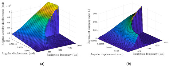
Figure 8.
Damper with a cubic nonlinear stiffness (). (a) Relative angular displacement and (b) equivalent damping ratio over the excitation frequency (natural frequency of the self-excited system) and angular displacement of the underlying structure (excitation frequency of the analytical system).
In contrast to a linear tuned mass damper (TMD), where a constant damping ratio occurs over the entire amplitude range but is only significantly high for a small frequency range, the nonlinear stiffness causes a shift of the characteristic frequency of the damper with the amplitude. At small amplitudes and, thus, small relative displacements between the structure and the damper, the dynamic motion of the nonlinear damper resembles that of the linear TMD. For higher amplitudes, the motion is affected significantly by the nonlinear stiffness and results in a frequency change. By harmonic linearization of the nonlinear stiffness [23,24,25], the linearized stiffness is calculated as a function of the amplitude:
resulting in the characteristic relative displacement:
that corresponds to the effective damping range of the nonlinear damper (maximum in Figure 8b). When the self-excitation frequency (excitation frequency of the analytical solution) is higher than the characteristic frequency of the linear part of the damper, an increase of the relative amplitude between the damper and structure results in a change of the effective frequency range of the nonlinear damper. This means that the effective frequency range of the nonlinear damper depends on the amplitude but is larger than the frequency range of a linear damper.
6.3. Comparison with Time Domain Simulations
The damping diagram in Figure 9a is derived by determining the equivalent damping ratio (Equation (52)) from the analytical solution (Equation (23)) for one natural frequency of the underlying self-excited structure (excitation frequency of the analytical solution). The natural frequency of the underlying structure is higher than the linear natural frequency of the damper to show the results regarding the nonlinear stiffness damper. In addition to the damping ratio provided by the damper, Figure 9a shows the absolute values of three different self-excited damping ratios. For two damping ratios and intersections occur between the self-excited absolute damping ratios and the damping provided by the damper. The highest negative damping ratio () exceeds the maximum additional damping provided by the damper. Figure 9b shows the relative displacement corresponding to the damper with respect to the amplitude of the underlying structure and the characteristic relative displacement (Equation (54)).
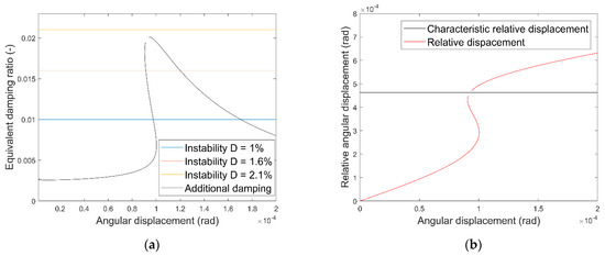
Figure 9.
Damper with a cubic nonlinear stiffness (). (a) Equivalent damping ratio regarding the angular displacement of the underlying structure. (b) Relative angular displacement regarding the angular displacement of the underlying structure.
For the smallest instability—thus, a linearized negative damping ratio of —the self-excited oscillation is limited and, thus, stabilized by the damping effect of the nonlinear damper. Due to the nonlinear stiffness and the frequency difference between the linear natural frequency of the damper and the vibration frequency of the structure, the damping effect is sufficient to stabilize the system above a certain amplitude. Therefore, at small amplitudes, the amplitude increases exponentially, as usual in self-excited systems (Figure 10a). At a certain amplitude, the damping ratio provided by the damper is sufficient to stabilize the self-excited system. The vibration amplitude of the structure is similar to the amplitude of the intersection in Figure 9a. As shown in Figure 8b the characteristic frequency and, thus, the damping is increased near the characteristic relative displacement. Due to the small, required damping ratio, the relative displacement does not exceed the characteristic relative displacement (Figure 10b).
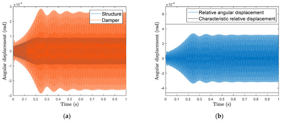
Figure 10.
Time domain results for an instability of (a) Angular displacement of the drill string structure and the damper. (b) Relative angular displacement between the damper and the drill string structure.
For higher self-excitations and, thus, higher negative damping ratios (), the intersection occurs at higher damping ratios. Figure 11a shows similar to Figure 10a at first an exponential increase of the amplitude at small relative displacements between the damper and the structure. The characteristic frequency of the nonlinear damper for this amplitude is below the vibration frequency of the structure. Due to the self-excitation, the amplitude, as well as the relative displacement between the damper and structure, increases. This increase of the relative displacement changes the characteristic frequency of the damper and, thus, increases its damping effect. This increased damping results in a reduction of the vibration amplitude of the structure. The smaller amplitude of the structure results in a smaller relative displacement and, thus, in a reduced damping effect. This repetitive increase and decrease of the amplitude and damping ratio results in a nonperiodic attractor (Figure 11a).
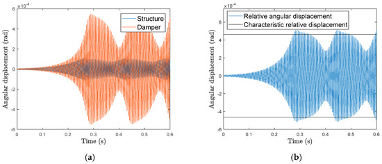
Figure 11.
Time domain results for an instability of (a) Angular displacement of the drill string structure and the damper. (b) Relative angular displacement between the damper and the drill string structure.
As Figure 11b shows, the relative displacement amplitude occurs around the characteristic relative amplitude. Similar to the self-excitation with , the amplitude of the structure is similar to the amplitude of the intersection in Figure 9a. For even higher self-excitations, e.g., , the additional damping is not sufficient to stabilize the unstable mode. Thus, an exponential increase of the amplitude occurs (Figure 12a,b). In Figure 12, a change in the dynamic motion of the structure regarding the characteristic frequency is visible at .
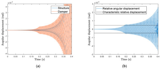
Figure 12.
Time domain results for an instability of (a) Angular displacement of the drill string structure and the damper. (b) Relative angular displacement between the damper and the drill string structure.
Figure 9a shows that the analytical results can be easily applied to self-excited structures. For self-excitations near the maximum of the damping ratio provided by the damper (e.g., in Figure 9a), the system is unstable, although according to the analytical solution, the system should be stabilized. Reasons for this small inaccuracy are the assumptions mentioned in Section 2 and Section 3, like the constant harmonic oscillation of the structure, the negligible reactive effect of the damper on the structure and the order of MSLP. One additional and very important reason is the combination of multiple possible occurring solitons in combination with the energy input and, thus, change of the amplitude in self-excited structures. This effect is shown in Figure 11. The damping effect is increased when the relative angular displacement is close to the characteristic relative angular displacement. The necessary relative displacement is achieved when the amplitude of the structural vibration increases.
This is seen well at higher natural frequencies of the self-excited structure, where the influence of the nonlinearity is high. Figure 13a shows the damping diagram when the natural frequency of the structure is increased to . Figure 13b shows that the instabilities of still resulted in a stable attractor due to the damping provided by the damper (similar to Figure 11). Figure 13a shows additionally to the damping diagram a principal depiction of the “closed loop” process, resulting in the attractor (Figure 13b). For a self-excited structure without significant shocks, the amplitude increases exponentially from a small initial amplitude. Due to the cubic stiffness nonlinearity of the system, the relative displacement and the corresponding damping ratio is low at small amplitudes and, thus, leads to an increase of the amplitude (Figure 13a arrow 1). At some point, an additional stable solution occurs, but the provided damping is low due to the initial small relative displacement (Figure 13a arrow 1). At higher amplitudes, the solution with small relative displacements disappears, and a rapid increase of the relative displacement between damper and structure leads to an increase of the provided damping (Figure 13a arrow 2). In Figure 13, the increased damping is sufficient to stabilize the instable mode and results in a decrease of the amplitude of the structure (Figure 13a arrow 3). This decrease of the structural amplitude leads to an increase of the provided damping and, thus, to an even faster decrease of the amplitude. Finally, the amplitude decreases below the amplitude of the maximum possible damping ratio, which causes the solution with high relative displacements and damping ratios to disappear (Figure 13a arrow 4). Due to the small relative displacement and damping ratio a repeated increase of the amplitude occurs (Figure 13a arrow 1). A slight increase of the instability to (Figure 14), although significantly below the theoretical maximum damping ratio, is unstable due to this change in amplitudes and relative displacements.
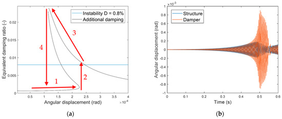
Figure 13.
Damper with a cubic nonlinear stiffness () and an instability of (a) Equivalent damping ratio regarding the angular displacement of the drill string structure. (b) Angular displacement of the drill string structure and the damper.
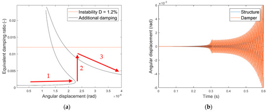
Figure 14.
Damper with a cubic nonlinear stiffness () and an instability of (a) Equivalent damping ratio regarding the angular displacement of the drill string structure. (b) Angular displacement of the drill string structure and the damper.
Again, beginning at the small amplitudes of the underlying structure, the relative displacement and the resulting additional damping is small (Figure 14a arrow 1). Due to the self-excitation, the amplitude increases similar to Figure 13a arrow 1 until the stable solution with small relative displacements disappears. This leads to a rapid increase of the relative displacement and provided damping (Figure 14a arrow 2). This effect is also visible in the time domain simulations in Figure 14b (. However, at these amplitudes, the maximum of the theoretically provided damping ratio is already exceeded, and the current damping is not sufficient to stabilize the unstable mode. Similar to Figure 12, the amplitude increases further (Figure 14a arrow 3 and Figure 14b ()), while the provided damping ratio decreases. This means that, in contrast to Figure 8, the maximum amplitude does not correlate with the occurring additional damping but, rather, the smallest stable amplitude.
6.4. Damper Design for Self-Excited Drill String Vibrations
The analytical results in Figure 8b with the theoretical maximum damping ratio are adjusted using the information about the stable and instable solutions and amplitude change (Figure 13 and Figure 14) to determine a realistic analytical solution (Figure 15).
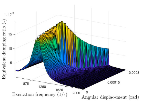
Figure 15.
Adjusted three-dimensional damping diagram of a damper with a cubic nonlinear stiffness ().
While Figure 8b shows the maximum theoretic damping ratio, Figure 15 shows the damping corresponding to the smallest stable amplitude. For self-excited systems, Figure 15 is very accurate, because self-excited vibrations that are not influenced by significant shocks or other special effects show an exponential increase of the amplitude, beginning at small amplitudes. As shown in Figure 13, this means that there is an increase in the amplitude and then a rapid increase from low relative displacements to high relative displacements and, thus, from low-to-high damping ratios. Using the analytical results (Section 3), the information on self-excited drill string vibrations (Equation (1)), the maximum amplitudes of high frequency vibrations (Equation (2)) and the transfer to self-excited vibrations (Figure 13, Figure 14 and Figure 15), it is now possible to efficiently design and optimize nonlinear dampers with respect to the critical drill string modes; the position within the drilling system and the design of the nonlinear damper in terms of inertia, damping and stiffness. The results obtained for the damper with cubic nonlinear stiffness are equally applicable to the other analytical solutions of the damper with cubic stiffness and friction. In addition, the results are transferable to other self-excited systems, where, for example, the reactive effect of the dampers on the dynamics of the structure is negligible due to, e.g., limited installation space.
7. Conclusions
In this paper, the Multiple Scales Lindstedt-Poincaré method was used to derive analytical solutions for two nonlinear dampers by using a specifically adapted drill string model. The advantages of the MSLP method compared to conventional methods like the Multiple Scales were discussed for this specific self-excited system. In this case, MSLP leads to exceptionally good results due to the frequency dependence of the excitation force in self-excited structure. The derived analytical solutions were transferred to self-excited drilling systems by analyzing the energy output and, thus, the stability of the considered self-excited drill string modes. In contrast to time-consuming time-domain simulations, the resulting equivalent damping ratio allows direct conclusions about the dynamic motion and stability of modes affected by dampers. Due to the variety of potentially critical modes (e.g., frequency and mode shape), of drill string and damper models (e.g., design and position) and the boundary conditions in deep drilling, such analytical solutions are essential for the effective design and optimization of dampers in deep drilling systems. In addition to the investigation of influencing parameters on the dynamic motion of the dampers, the analytical results are simulatively validated using self-excited drill string models. The influence of the nonlinear stiffness on the stability and shape of the resulting attractors is shown, and three representative dynamic responses of the self-excited structure were discussed. The equations derived from the analytical solutions with the aim of mitigating critical drill string vibrations. The procedure described above is transferable to other fields of engineering where similar conditions, such as low reactive effects, occur. The presented method and the derived analytical solutions will further be used for the efficient design and optimization of nonlinear dampers. Furthermore, the complex nature of self-excitation due to bit-rock interaction with various uncertainties can be addressed in more detail in the future.
Author Contributions
Conceptualization, V.K. and G.-P.O.; data curation, V.K. and P.T.; formal analysis, V.K. and P.T.; funding acquisition, G.-P.O.; investigation, V.K. and P.T.; methodology, V.K.; project administration, F.S. and G.-P.O.; resources, G.-P.O.; software, V.K. and P.T.; supervision, G.-P.O.; validation, V.K. and P.T.; visualization, V.K., P.T. and G.-P.O.; writing—original draft, V.K. and P.T.; writing—review and editing, F.S. and G.-P.O. All authors have read and agreed to the published version of the manuscript.
Funding
We acknowledge support by the Open Access Publication Funds of the TU Braunschweig.
Acknowledgments
The authors would like to thank Baker Hughes for supporting the work and giving permission to publish this paper.
Conflicts of Interest
The authors declare no conflict of interest.
References
- Reckmann, H.; Jogi, P.; Kpetehoto, F.T.; Chandrasekaran, S.; Macpherson, J.D. MWD Failure Rates Due to Drilling Dynamics. In Proceedings of the IADC/SPE Drilling Conference and Exhibition, New Orleans, LA, USA, 2–4 February 2010; Society of Petroleum Engineers: Richardson, TX, USA, 2010. [Google Scholar]
- Bowler, A.I.; Logesparan, L.; Sugiura, J.; Jeffryes, B.P.; Harmer, R.J.; Ignova, M. Continuous High-Frequency Measurements of the Drilling Process Provide New Insights into Drilling System Response and Transitions between Vibration Modes. In Proceedings of the SPE Annual Technical Conference and Exhibition, Amsterdam, The Netherlands, 27 October 2014; Society of Petroleum Engineers: Richardson, TX, USA, 2014. [Google Scholar]
- Cunningham, R.A. Analysis of Downhole Measurements of Drill String Forces and Motions. J. Eng. Ind. 1968, 90, 208–216. [Google Scholar] [CrossRef]
- Dareing, D.W.; Livesay, B.J. Longitudinal and Angular Drill-String Vibrations with Damping. J. Eng. Ind. 1968, 90, 671–679. [Google Scholar] [CrossRef]
- Hohl, A.; Kulke, V.; Kueck, A.; Heinisch, D.; Herbig, C.; Ostermeyer, G.-P.; Reckmann, H. Best Practices for Operations in HFTO Prone Applications. Available online: https://onepetro.org/SPEAPOG/proceedings-abstract/20APOG/3-20APOG/D033S024R001/451737 (accessed on 9 February 2021).
- Ritto, T.G.; Soize, C.; Sampaio, R. Probabilistic model identification of the bit–rock-interaction-model uncertainties in nonlinear dynamics of a drill-string. Mech. Res. Commun. 2010, 37, 584–589. [Google Scholar] [CrossRef]
- Fu, C.; Xu, Y.; Yang, Y.; Lu, K.; Gu, F.; Ball, A. Response analysis of an accelerating unbalanced rotating system with both random and interval variables. J. Sound Vib. 2020, 466, 115047. [Google Scholar] [CrossRef]
- Hohl, A.; Tergeist, M.; Oueslati, H.; Jain, J.R.; Herbig, C.; Ostermeyer, G.-P.; Reckmann, H. Derivation and experimental validation of an analytical criterion for the identification of self-excited modes in drilling systems. J. Sound Vib. 2015, 342, 290–302. [Google Scholar] [CrossRef]
- Zhang, Z.; Shen, Y.; Chen, W.; Shi, J.; Bonstaff, W.; Tang, K.; Smith, D.L.; Arevalo, Y.I.; Jeffryes, B. Continuous High Frequency Measurement Improves Understanding of High Frequency Torsional Oscillation in North America Land Drilling. In Proceedings of the SPE Annual Technical Conference and Exhibition, San Antonio, TX, USA, 9 October 2017; Society of Petroleum Engineers: Richardson, TX, USA, 2017. [Google Scholar]
- Ledgerwood, L.W.; Hoffmann, O.J.-m.; Jain, J.R.; El Hakam, C.; Herbig, C.; Spencer, R. Downhole Vibration Measurement, Monitoring, and Modeling Reveal Stick/Slip as a Primary Cause of PDC-Bit Damage in Today. In Proceedings of the SPE Annual Technical Conference and Exhibition, Florence, Italy, 19 September 2019; Society of Petroleum Engineers: Richardson, TX, USA, 2010. [Google Scholar]
- Pastusek, P.E.; Sullivan, E.; Harris, T.M. Development and Utilization of a Bit Based Data Acquisition System in Hard Rock PDC Applications. In Proceedings of the SPE/IADC Drilling Conference, Amsterdam, The Netherlands, 20 February 2007; Society of Petroleum Engineers: Richardson, TX, USA, 2007. [Google Scholar]
- Dennis, H.; Mathäus, W.; Christian, H.; Andreas, H.; Hanno, R. High-Frequency Torsional Oscillation Laboratory Testing of an Entire Bottom Hole Assembly. In Proceedings of the Abu Dhabi International Petroleum Exhibition & Conference, Abu Dhabi, United Arab Emirates, 13 November 2017; Society of Petroleum Engineers: Richardson, TX, USA, 2017. [Google Scholar]
- Heinisch, D.; Kulke, V.; Peters, V.; Hohl, A.; Schepelmann, C.; Reckmann, H.; Ostermeyer, G.-P. Simulation and Testing of an Isolator Tool for High-Frequency Torsional Oscillation. In Proceedings of the Abu Dhabi International Petroleum Exhibition & Conference, Abu Dhabi, United Arab Emirates, 12 November 2018; Society of Petroleum Engineers: Richardson, TX, USA, 2018. [Google Scholar]
- Jain, J.R.; Oueslati, H.; Hohl, A.; Reckmann, H.; Ledgerwood III, L.W.; Tergeist, M.; Ostermeyer, I.h.G.-P.; Ostermeyer, G.P. High-Frequency Torsional Dynamics of Drilling Systems: An Analysis of the Bit-System Interaction. In Proceedings of the IADC/SPE Drilling Conference and Exhibition, Fort Worth, TX, USA, 4 March 2014; Society of Petroleum Engineers: Richardson, TX, USA, 2014. [Google Scholar]
- Oueslati, H.; Jain, J.R.; Reckmann, H.; Ledgerwood, L.W.; Pessier, R.; Chandrasekaran, S. New Insights into Drilling Dynamics Through High-Frequency Vibration Measurement and Modeling. In Proceedings of the SPE Annual Technical Conference and Exhibition, New Orleans, LA, USA, 30 September 2013; Society of Petroleum Engineers: Richardson, TX, USA, 2013. [Google Scholar]
- Hohl, A.; Tergeist, M.; Oueslati, H.; Herbig, C.; Ichaoui, M.; Ostermeyer, G.-P.; Reckmann, H. Prediction and Mitigation of Torsional Vibrations in Drilling Systems. In Proceedings of the IADC/SPE Drilling Conference and Exhibition, Fort Worth, TX, USA, 1 March 2016; Society of Petroleum Engineers: Richardson, TX, USA, 2016. [Google Scholar]
- Hohl, A.; Herbig, C.; Arevalo, P.; Reckmann, H.; Macpherson, J. Measurement of Dynamics Phenomena in Downhole Tools - Requirements, Theory and Interpretation. In Proceedings of the IADC/SPE Drilling Conference and Exhibition, Fort Worth, TX, USA, 6 March 2018; Society of Petroleum Engineers: Richardson, TX, USA, 2018. [Google Scholar]
- Andreas, H.; Eric, P.; Pedro, A. Real-Time System to Calculate the Maximum Load of High-Frequency Torsional Oscillations Independent of Sensor Positioning. In Proceedings of the SPE/IADC International Drilling Conference and Exhibition, Hague, The Netherlands, 4 March 2019; Society of Petroleum Engineers: Richardson, TX, USA, 2019. [Google Scholar]
- Hohl, A.; Kulke, V.; Kueck, A.; Herbig, C.; Reckmann, H.; Ostermeyer, G.-P. The Nature of the Interaction Between Stick/Slip and High-Frequency Torsional Oscillations. In Proceedings of the IADC/SPE International Drilling Conference and Exhibition, Galveston, TX, USA, 25 February 2020; Society of Petroleum Engineers: Richardson, TX, USA, 2020. [Google Scholar]
- Tondl, A. Quenching of self-excited vibrations equilibrium aspects. J. Sound Vib. 1975, 42, 251–260. [Google Scholar] [CrossRef]
- Tondl, A. Quenching of self-excited vibrations: Effect of dry friction. J. Sound Vib. 1976, 45, 285–294. [Google Scholar] [CrossRef]
- Kulke, V.; Ostermeyer, G.-P.; Tergeist, M.; Hohl, A. Semi-Analytical Approach for Derivation of an Equivalent Modal Friction-Damping Ratio and its Application in a Self-Excited Drilling System. In Volume 4: Dynamics, Vibration, and Control, Proceedings of the ASME 2019 International Mechanical Engineering Congress and Exposition, Salt Lake City, UT, USA, 11–14 November 2019; American Society of Mechanical Engineers: New York, NY, USA, 2019; ISBN 978-0-7918-5941-4. [Google Scholar]
- Kim, W.-J.; Perkins, N.C. Harmonic balance/Galerkin method for non-smooth dynamic systems. J. Sound Vib. 2003, 261, 213–224. [Google Scholar] [CrossRef]
- Krack, M.; Gross, J. Harmonic Balance for Nonlinear Vibration Problems; Springer International Publishing: Cham, Switzerland, 2019; ISBN 978-3-030-14022-9. [Google Scholar]
- Nakhla, M.; Vlach, J. A piecewise harmonic balance technique for determination of periodic response of nonlinear systems. IEEE Trans. Circuits Syst. 1976, 23, 85–91. [Google Scholar] [CrossRef]
- Nayfeh, A.H.; Mook, D.T. Nonlinear Oscillations; Wiley: New York, NY, USA, 1979; ISBN 0-471-03555-6. [Google Scholar]
- Nayfeh, A.H. Resolving Controversies in the Application of the Method of Multiple Scales and the Generalized Method of Averaging. Nonlinear Dyn. 2005, 40, 61–102. [Google Scholar] [CrossRef]
- Pakdemirli, M.; Karahan, M.M.F.; Boyacı, H. A New Perturbation Algorithm With Better Convergence Properties: Multiple Scales Lindstedt Poincare Method. MCA 2009, 14, 31–44. [Google Scholar] [CrossRef]
- Pakdemirli, M.; Sarı, G. Solution of Quadratic Nonlinear Problems with Multiple Scales Lindstedt-Poincare Method. MCA 2015, 20, 137–150. [Google Scholar] [CrossRef]
Publisher’s Note: MDPI stays neutral with regard to jurisdictional claims in published maps and institutional affiliations. |
© 2021 by the authors. Licensee MDPI, Basel, Switzerland. This article is an open access article distributed under the terms and conditions of the Creative Commons Attribution (CC BY) license (http://creativecommons.org/licenses/by/4.0/).