A Study on the Dynamic Behavior of a Vertical Tunnel Shaft Embedded in Liquefiable Ground during Earthquakes

Abstract

Since liquefaction was first observed in South Korea during the Pohang earthquake, public concerns regarding the seismic stability of major infrastructure have increased substantially. However, the seismic behavior of tunnel shafts, which are an important element of tunnel structures, has not been properly established, especially under liquefiable soil conditions. In this study, 3D numerical modeling with Fast Lagrangian Analysis of Continua in 3 Dimensions (FLAC3D) was performed to predict the dynamic behavior of a vertical tunnel shaft during liquefaction. This study demonstrates key aspects of the dynamic behavior of tunnel shafts by varying important parameters such as the thickness of the liquefiable soil layer and applied seismicity level. Moreover, important dynamic responses such as excess pore pressure generation, the seismic bending moment of the shaft, and lateral displacements are highlighted. Finally, meaningful discussion of the seismic risk analysis based on damage indices is conducted based on the analysis results.

1. Introduction

Liquefaction is a major cause of damage to facility structures during earthquakes; it was first observed in South Korea during the Pohang earthquake. As a result, public concern regarding the seismic stability of major infrastructure has been increasing, and revision of the seismic design criteria for various facilities is in progress. As summarized in Kwon & Yoo (2020) [1], behavior of the soil-pile system in in liquefiable sand exhibits more complicated characteristics than that in dry soil due to the development of excess pore pressure caused by cyclic loading. Once earthquake occurs, the seismic wave originating from the bedrock causes cyclic underground shear stress as it is propagated to the upper soil. Such shear stress leads to shear deformation of the soil, thereby increasing the pore pressure of the soil. This increase in pore pressure decreases the effective stress of the soil, and liquefaction occurs when the generated excess pore pressure equals the initial effective stress of the soil. In this case, soil completely loses its shear strength and exhibits behavior similar to that of water. Therefore, it is crucial to accurately predict liquefaction potential and the structural behavior of foundations in the event of liquefaction to prevent damage to the structures. Several researchers such as Cavallaro et al. [2], Idriss & Boulanger [3], and Idriss [4] have proposed various types of methodology to evaluate liquefaction potential by in situ test, lab test, semi-empirical procedures, etc.

As underground structures in liquefiable sand have more complex performance mechanisms than those in non-liquefiable soil, these structures exhibit more uncertain and unpredictable characteristics. In liquefiable soil conditions, not only does the inertial force of the upper structure and the kinematic force due to soil deformation apply different dynamic loads on the underground structure, but the stiffness and shear strength of the soil also decrease over time owing to the nonlinear behavior of soil and the development of excess pore pressure.

Tunnels are frequently used underground structures for roads, railways, metro systems, etc. Major tunnels that are long and are located near urban areas usually have vertical shafts for both ventilation and possible emergencies. The role of the tunnel shaft is critical for safety and the indoor environment, but seismic consideration of the shaft structure is more limited than that of the main tunnel body. Unlike the tunnel body, the dynamic behavior of the tunnel shaft can be critically influenced by the ground condition because it is usually installed vertically from the ground surface to the tunnel body. In addition, these tunnel shafts also frequently have relatively slender shapes in the vertical direction.

Sevim [5], Fattah et al. [6], Liu et al. [7], and Lee et al. [8] investigated the dynamic responses of tunnels under earthquake loading using numerical analyses. Liu et al. [9] performed shaking table model tests to investigate the mechanism and effect of seismic loading on a horseshoe-scaled tunnel model at a ground fissure site. Schmidt and Hashash [10], Chou et al. [11], Adalier et al. [12], Chang et al. [13], Azadi and Hosseini [14], Bao et al. [15], Lee et al. [16], Miranda et al. [17], and Sugito et al. [18] analyzed the dynamic behavior of tunnels embedded in liquefiable soil using model tests or numerical analyses. However, these studies mainly focused on the uplifting of the tunnel under liquefaction, damage to the tunnel body, and tunnel–building interaction problems. Thus, research on the seismic behavior of tunnel shafts, which are an important element of the tunnel structure, is very limited. Only a few studies have been conducted on tunnel shafts. Meyoral et al. [19] suggested a numerical approach to derive fragility curves for tunnel shafts built in clays. Yu et al. [20] analyzed the dynamic response of a long tunnel and tunnel shaft during an earthquake using a multi-scale method. However, these studies did not consider liquefaction or liquefiable soil characteristics. Liquefaction usually occurs in loose sandy soils that tunnel shafts often pass through, and it can induce a remarkable amount of kinematic force on the shaft body depending on the ground and input earthquake conditions. Therefore, an appropriate investigation of the seismic performance of a tunnel shaft under liquefiable soil conditions is needed to obtain a safe and sustainable seismic design of the entire tunnel system.

In this study, three-dimensional numerical modeling was performed to predict the dynamic behavior of a vertical tunnel shaft that passes through a liquefiable loose sand layer. Important parameters such as the thickness of the liquefiable sand layer and input earthquake magnitude were varied and used for the analysis of 12 different cases. The seismicity levels of artificially described earthquake records were defined to reflect the revised Korean seismic design criteria [21]. Fast Lagrangian Analysis of Continua in 3 Dimensions (FLAC3D) was used as the simulation tool, and detailed dynamic soil properties and shaft properties were determined based on preliminary analyses and typical conditions. The input earthquake motions were input at the base of the model and artificially defined based on Pohang earthquake records. The upper sand layer was completely saturated and sufficiently loose to liquefy under the applied earthquake levels. This study highlights the key aspects of the seismic behavior of a tunnel shaft under liquefaction, such as excess pore pressure generation and the seismic bending moment, and displacement of the shaft, and provides a meaningful discussion regarding earthquake risk assessment with damage indices based on the analysis results.

2. Modeling Methodology and Conditions

In this study, the seismic responses of a tunnel shaft during liquefaction were simulated using FLAC3D (Fast Lagrangian Analysis of Continua in 3 Dimensions) [22], which is a three-dimensional numerical simulation tool. The model system was virtually defined based on typical construction conditions of urban railway tunnels in Seoul, South Korea. The model tunnel of an urban railway (prototype) was located in the rock layer. A vertical shaft structure fabricated from reinforced concrete was rigidly installed at the top side of the tunnel body. A liquefiable loose sand layer was located above the rock layer, and the model shaft penetrated both layers vertically from the top side of the tunnel body. The primary dimensions and material properties of the tunnel shaft structure are presented in

Table 1. Material properties of the tunnel shaft.

Material Properties	Value
Outer diameter (m)	5
Concrete stiffness (MPa)	24
Elastic modulus of concrete(MPa)	26,950
Steel stiffness (MPa)	300
Inner diameter (m)	4.6
Elastic modulus of steel(MPa)	200,000
Unit weight of reinforced concrete (kN/m3)	25
Poisson’s ratio	0.33

. The 12 analysis cases were composed of four depths of the base rock (5 m, 10 m, 15 m, and 21 m), i.e., thicknesses of the liquefiable layer, and three amplitudes of the input earthquake motion (500 y, 1000 y, and 2400 y), as summarized in

Table 2. List of analysis cases considered in this study.

Case Number
	Depth of the base rock (m)	Return period of the input earthquake motion (y)
1	5 m	500
2		1000
3		2400
4	10 m	500
5		1000
6		2400
7	15 m	500
8		1000
9		2400
10	21 m	500
11		1000
12		2400

and Figure 1.

A soil constitutive model for liquefiable soil should be able to simulate important dynamic behaviors such as pore water pressure generation and reduction in effective strength during liquefaction. In the present study, the Finn liquefaction model was adopted, which has been verified through comparison with various field observations and model tests in several previous studies [23,24,25,26]. The Finn model correlates the increment of the volumetric strain per loading cycle $\Delta {\epsilon }_{vd}$ with increase in the shear strain amplitude $\mathsf{\gamma }$ during that particular cycle. The Finn model was incorporated into the Mohr–Coulomb plasticity model. For practical purposes, Byrne [27] proposed simple equations to determine these parameters as functions of the relative density of sand, as shown in Equations (1) and (2):

$$\frac{\Delta {\epsilon }_{vd}}{\mathsf{\gamma }}=C_1\exp (-C_2\left(\frac{{\epsilon }_{vd}}{\gamma }\right))$$

(1)

$$C_1=7600{\left(D_r\right)}^{-2.5},{ \mathrm{C}}_2=\frac{0.4}{C_1}$$

(2)

where ${\epsilon }_{vd}$ is the accumulated irrecoverable volumetric strain to the Nth cycle, $\gamma$ is the shear strain at the (N + 1)th cycle, $\Delta {\epsilon }_{vd}$ is the increment of the volume decrease at the (N + 1)th cycle, and $C_1$ and $C_2$ are volume change constants.

The nonlinearity of soil significantly influences the dynamic behavior of the shaft. In this study, the hysteretic damping model was applied to consider both the nonlinear variations in the shear modulus and damping ratio and the energy dissipation. This model presents the G/G_max curve versus the logarithm of the cyclic strain and the tangent modulus as shown in Equations (3)–(5).

$$M_t=s^2\left(3-2s\right)-\frac{6s\left(1-s\right)}{L_2-L_1}{\log }_{10}\exp$$

(3)

$$\mathrm{L}={\log }_{10}\left(\gamma \right)$$

(4)

$$\mathrm{s}=\frac{L_2-L}{L_2-L_1}$$

(5)

where $M_t$ is the tangent modulus, L is the logarithmic strain, and $L_1 \mathrm{and} L_2$ and are the extreme values of L.

$L_1$ and $L_2$ represent the degradation rate and starting point of the degradation of G/G_max curve, respectively. $L_1$ and $L_2$ for the model soil were set as −3.65 and 0.5, respectively, as proposed by Kwon and Yoo [28]. The maximum shear modulus of the soil, G_max, was calculated using Equation (6), as proposed by Hardin and Drnevich [29].

$$G_{max}=AF\left(e\right){\left(OCR\right)}^k{P}_a{}^{1-n}{\left({{\sigma }^{\prime }}_m\right)}^n$$

(6)

where F(e) = 1/(0.3 + 0.7e²), in which e is the void ratio; ${{\sigma }^{\prime }}_m$ is the mean principal effective stress; $P_a$ is the atmospheric pressure; k is the overconsolidation ratio exponent (which is equal to 0 in sand); and A and n are empirical coefficients, which were determined to have values of 247.73 and 0.567, respectively, for model soil [28].

An interface element that allows both slippage and separation between the soil and the shaft structure under strong earthquake loading was applied to simulate the dynamic soil–structure interaction. The interface model attaches normal and shear springs with equivalent spring stiffness between the soil and shaft, as shown in Equation (7) [1]. In Equation (7), G reflects the nonlinear reduction in the soil shear stiffness; therefore, the nonlinear behavior at the interface can also be captured in the proposed model.

$$K_E=max\left[\frac{K+\left(4/3\right)G}{\Delta z_{min}}\right]$$

(7)

where $K_E$ is the equivalent stiffness of the interface spring; K and G are the bulk and shear moduli of the soil, respectively; and $\Delta z_{min}$ is the smallest width of an adjoining zone in the normal direction.

One of the important points for modeling soil–structure systems under dynamic conditions is the proper simulation of the free-field boundary. Improper boundary conditions in dynamic simulations can cause the reflection of outward propagating waves back into the model and do not allow for the necessary energy radiation. Therefore, in this study, the free-field boundary model implemented in FLAC3D was used along the edge of the model. The free-field boundary is used to enforce the free-field motion such that the boundaries retain their non-reflecting properties and outward waves originating from the structure are properly absorbed.

The input properties of the model soil used in the numerical simulation were determined based on typical values for Jumunjin sand, which is a Korean standard sand, as summarized in

Table 3. Material properties of the model soil.

Material Properties	Value
Void ratio	0.95
Poisson’s ratio	0.3
Dry density (kN/m3)	13.8
Friction angle (°)	32
Cohesion (kN/m2)	0
Relative density (%)	30

and

Table 4. Material properties of the base rock.

Material Properties	Value
Unit weight (kN/m3)	23
Elastic modulus (kN/m2)	3,600,000
Friction angle (°)	42
Cohesion (kN/m2)	300

.

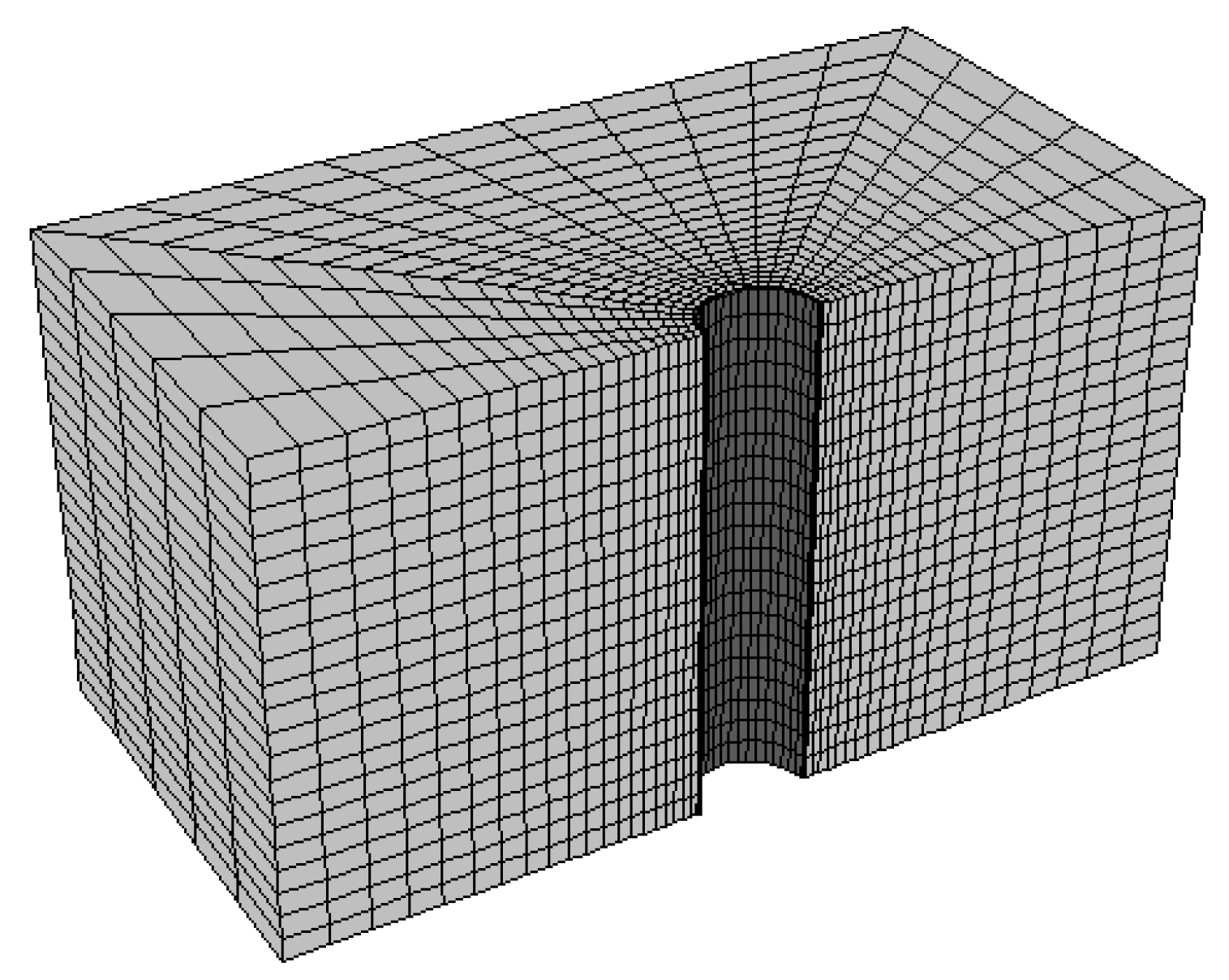
The model soil was defined as liquefiable loose sand and was completely saturated in the model. Figure 2 shows a representative modeling mesh of the target system (Cases 10, 11, and 12) used to calculate seismic responses of the tunnel shaft in this study. In this figure, only half of the system was modeled for efficiency of the analysis; the entire system can be obtained by reflection in the simulation tool. The geometry of the tunnel and rock layer was omitted in the analysis model and the input earthquake motion was directly induced at the base of the model because the shaft and tunnel in the rock layer were regarded as fully fixed. The shaft structure was modeled using a cylinder-type solid element with an elastic model. Dynamic analysis was then carried out based on a three-dimensional finite difference approach. The analysis proceeded via the following steps according to the construction and loading phases: (1) static equilibrium of the soil media, (2) construction of the tunnel shaft and attainment of static equilibrium of the overall system, and (3) dynamic analysis.

The input earthquake motion used in this study was artificially created based on recorded values from the Pohang earthquake, and the spectrum amplitude was calibrated using the Korean standard response spectrum announced in 2017. Three types of input earthquake motions were estimated according to the return period (500, 1000, and 2400 y), with maximum acceleration values of 0.136 g, 0.190 g, and 0.272 g, respectively. Input motions were induced at the bottom level of the model in the form of acceleration time histories. The profiles of the earthquake motions used in this study are shown in Figure 3.

3. Results of the Numerical Simulations

Figure 4 shows the calculated excess pore pressure ratio time histories for two different depths in Cases 2 and 3. In both cases, the excess pore pressure ratio reached 1.0 at a depth of −1.5 m and gradually decreased with increasing depth to −4.5 m. The excess pore pressure increased sharply at approximately 5–6 s in each case, which is a similar trend to that of the input earthquake motion. The fluctuation in the pore pressure response was more significant in Case 3, demonstrating that the volumetric strain and variation in the stress state were more prominent in stronger earthquakes. The excess pore pressure ratio at −4.5 m for Case 2 was lower than that for Case 3 because of the difference in the amplitude of the input earthquake. This indicates that liquefaction occurred at a deeper depth when a stronger earthquake was induced for identical ground conditions. Figure 5 shows the excess pore pressure ratio time histories calculated for two different depths in Cases 11 and 12. At a depth of −9.5 m, 100% liquefaction occurred in Case 12, whereas almost 50% liquefaction occurred in Case 11. At a depth of −5.5 m, 100% liquefaction occurred in both cases. This is a similar trend to that of Cases 2 and 3 in Figure 4. However, the liquefied area was much deeper in Cases 11 and 12 than in Cases 2 and 3. It can be predicted that much more kinematic interaction would be induced in Cases 11 and 12 than in Cases 2 and 3.

Table 5. Range of maximum depth at which the excess pore pressure reached 1.0.

Case No.	Depth at Which ue = 1.0 (m)	Case No.	Depth at Which ue = 1.0 (m)
Case 1	1.5–2.0	Case 7	6.0–6.5
Case 2	2.0–2.5	Case 8	6.5–7.0
Case 3	2.5–3.0	Case 9	7.5–8.0
Case 4	2.5–3.0	Case 10	7.5–8.0
Case 5	4.0–4.5	Case 11	8.0–8.5
Case 6	5.0–5.5	Case 12	9.5–10.0

presents the ranges of the maximum depth at which the excess pore pressure ratio reached 1.0 for each analysis case. It shows that as the thickness of the liquefiable layer increased and the input seismicity increased, the depth at which the excess pore water pressure ratio reached 1.0 also increased. It also demonstrated that the magnitude of the input earthquake and the seismic site have a significant effect on the level of liquefaction, and it is expected that this phenomenon will affect the dynamic behavior of the shaft structure.

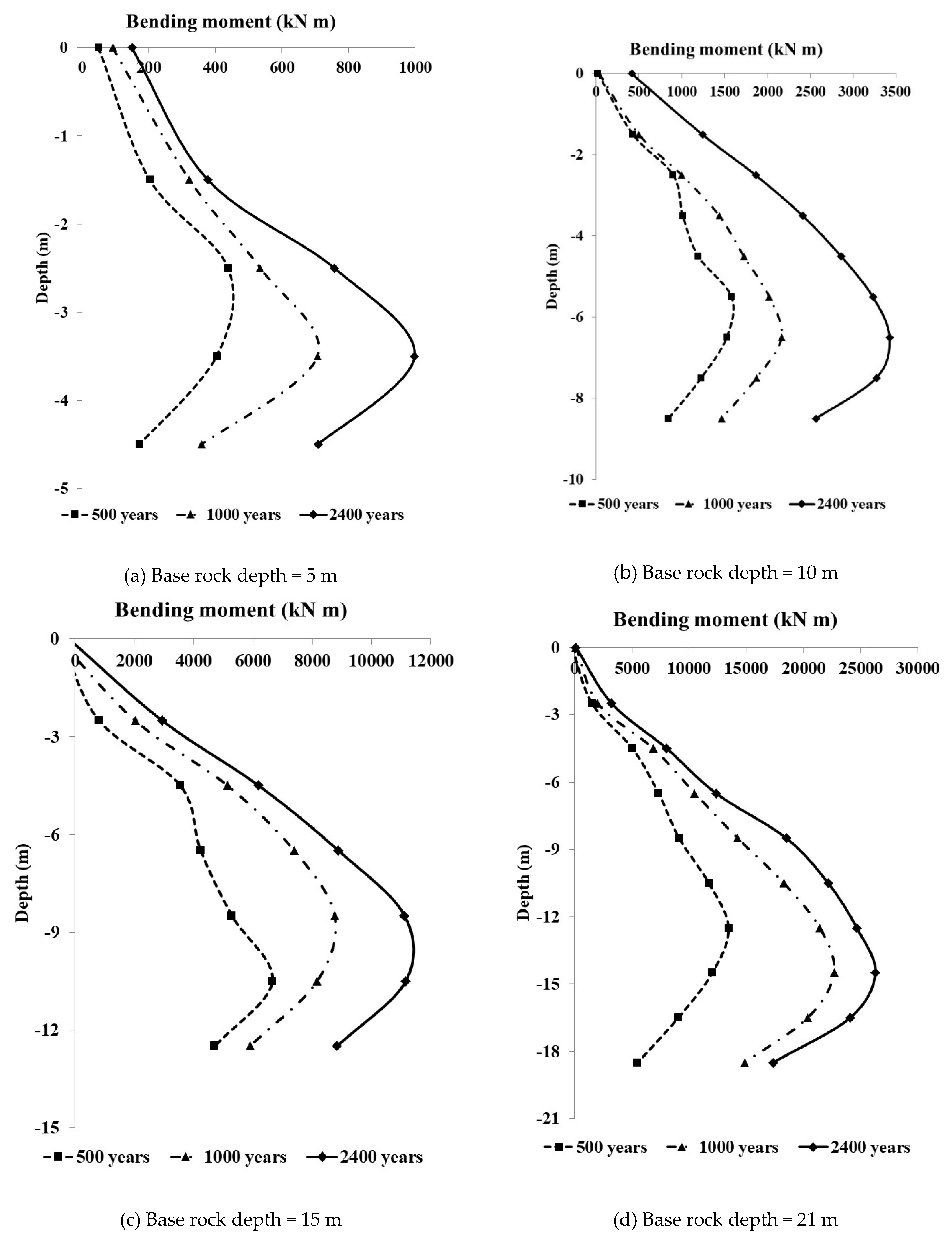
Figure 6 shows peak bending moment profiles for the shaft along the depth in each analysis case. As shown in this figure, the bending moments for the cases with longer earthquake return periods were generally larger than those for the cases with shorter earthquake return periods. The peak bending moment measured for the earthquake with a 2400 y return period was almost 2.5 times larger than that for the earthquake with a 500 y return period. In addition, the calculated dynamic bending moment increased as the bedrock depth increased. The peak bending moments for cases with a bedrock depth of 21 m were almost 25 times larger than those for cases with a bedrock depth of 5 m. This indicates that the kinematic force induced by liquefaction at deeper soil depths has a significant influence on the dynamic shaft behavior. The location at which the peak bending moment occurred was deeper than the center of the total depth. In addition, the location at which the peak bending moment occurred became deeper with an increase in the earthquake return period. This indicates that stronger earthquakes produced larger liquefied areas, and that greater kinematic force induced by liquefaction was exerted on the shaft structure.

Figure 7 shows a representative graph of the lateral displacement time histories for the shaft and far-field soil. The shaft and soil behaved in-phase for the entire earthquake duration. This means that the shaft behavior was governed by the soil behavior, which was induced by kinematic interaction. In addition, the residual displacement of the soil at the surface was larger than that of the shaft. This phenomenon could indicate the occurrence of relative displacement after liquefaction.

Figure 8 shows the maximum lateral shaft and soil displacement profiles along the depth for Cases 5 and 11. The lateral displacement was slightly greater in Case 11 than Case 5; however, the discrepancy was smaller than that of the bending moment. In addition, the lateral displacement profiles for the far-field soil were very similar to those for the shaft. It should be noted that the kinematic performance is the dominant factor for the liquefaction condition. The maximum displacement of the shaft and soil reached almost 1% of the shaft diameter. This indicates that the displacement caused by liquefaction did not exceed the elastic range.

Figure 9 shows the residual lateral shaft and soil displacement profiles along the depth for Cases 5 and 11. The residual displacements of the far-field soil were larger than the lateral shaft displacements. Both residual displacements increased with the depth of the base rock. In addition, relative displacements also occurred in both cases. This indicates that a gapping phenomenon could occur between the soil and shaft after liquefaction, although the implicit value is very small.

4. Structural Integrity of the Shaft under Liquefaction

The allowable bending moment of the shaft was calculated using a sectional analysis in Response2000 [30]. The input geometric properties are summarized in

Table 6. Material properties of the model concrete shaft.

	Gross Conc.	Trans (n = 7.54)
Area (mm2)	3.07 × 106	3.12 × 106
Inertia (mm4)	8.9 × 1012	9.1 × 1012
yt (mm)	2500	2500
yb (mm)	2500	2500
st (mm3)	3.57 × 1012	3.63 × 1012
Sb (mm3)	3.57 × 1012	3.63 × 1012

. Based on the sectional analysis results, the cracking moment and maximum allowable moment were determined as 6438 kN·m and 10,467 kN·m, respectively.

To evaluate the earthquake risk assessment for a tunnel shaft, the maximum moment value obtained from the numerical analysis was compared with the calculated cracking moment. The damage state of the underground structure could be classified into three states: minor/slight, moderate, and extensive. Argyroudis and Pitilakis [31] suggested a damage index applying the failure moment (Md) and measuring moment. In addition, a damage state using the ratio of the measuring moment to the yielding moment (My) was developed by Park et al. [32]. When the damage state was determined using the Md value, the predicted damage state was significantly more conservative than the actual seismic performance. Therefore, in this study, My was applied to determine the damage state and consider the performance uncertainty of a reinforced concrete structure [32]. The My value was referred to in the cracking moment from the sectional analysis. The damage states defined in previous research are summarized in

Table 7. Damage states.

Damage State	Damage Index, M/Md (Argyroudis and Pitilakis (2012))	Damage Index M/My (Park et al. (2016))
None	DI < 1.0	DI < 1.0
Minor/slight	1.0 < DI < 1.5	1.0 < DI < 1.4
Moderate	1.5 < DI < 2.5	1.4 < DI < 2.3
Extensive	2.5 < DI <3.5	2.3 < DI

.

The maximum moment values from the numerical analysis are summarized in

Table 8. Maximum moments of the tunnel shaft in the numerical analysis results (kN.m).

Depth of Liquefiable Soil Deposit	Return Period of the Earthquake
	500 y	1000 y	2400 y
5 m	439	707	998
10 m	1582	2168	3428
15 m	6654	8767	11,155
21 m	13,455	22,678	26,298

. In addition, based on the numerical analysis results, damage index values were calculated for each case using the damage states developed by Park et al. [29]. Figure 10 shows the damage index results for each case. The maximum observed moment value was lower than the cracking moment for liquefiable deposit depths of 5 m and 10 m, and no damage states were expected. However, the shaft structure with a liquefiable layer of 15 m could experience slight damage under earthquakes with return periods of 500 and 1000 y. In addition, a moderate damage state could be produced under an earthquake having a return period of 2400 y. In the case of the shaft with a 21 m liquefiable layer, the damage index values for all cases were greater than 1.4, indicating that at least moderate damage could occur in the shaft structure with deep liquefiable deposits. In particular, the damage index of Cases 11 and 12 exceeded values of 2.3, which implies that extensive damage could occur under an earthquake with a return period of 1000 y.

To evaluate the seismic risk of the shaft structure, a risk assessment framework was constructed based on the damage index analysis results for the bending moment. The rows are the return periods of the earthquake, which denotes the hazard intensity, and the columns are the case numbers, which indicate the thickness of the liquefiable layer. The case number of numerical analysis is summarized in

Table 9. Numerical analysis cases.

Return Period of Earthquake	Depth of Liquefiable Soil Deposit
	5 m	10 m	15 m	21 m
500 years	Case 1	Case 4	Case 7	Case 10
1000 years	Case 2	Case 5	Case 8	Case 11
2400 years	Case 3	Case 6	Case 9	Case 12

. As shown in Figure 11, the risk index is more severe with increasing hazard intensity, and the risk index also increases with an increasing depth of the base rock.

The structures with liquefiable layer thicknesses of 5 m and 10 m were mostly safe regardless of the hazard intensity. In the cases with a liquefiable layer thickness of 15 m, the shaft structure could suffer moderate damage under an increased hazard intensity. The shaft structure with a liquefiable layer thickness of 21 m has the possibility of suffering more than moderate damage regardless of the hazard intensity. Therefore, it is necessary to consider the liquefaction risk not only in underground structures such as tunnels and stations but also in shaft structures, especially those installed at depths of greater than 15 m.

5. Conclusions

The dynamic behavior of a tunnel shaft during liquefaction was investigated by numerically obtaining the seismic response of the target system. The following are detailed concluding remarks.

(1) The model system was defined virtually based on typical construction conditions for urban railway tunnels in South Korea. Seismic responses of vertical tunnel shafts that pass through a liquefiable loose sand layer were simulated using FLAC3D for 12 analysis cases with varying liquefiable sand layer thicknesses (5, 10, 15, and 21 m) and input earthquake motion return periods (500, 1000, and 2400 y).

(2) The Finn liquefaction model was adopted for the soil constitutive model. Interface elements, free-field boundaries, and hysteretic damping were properly incorporated into the soil model to simulate the dynamic soil–structure interaction under strong earthquake conditions. The input earthquake motion was artificially created based on recorded values from the Pohang earthquake (M5.4, 2017).

(3) As the thickness of the liquefiable layer increased and the input seismicity increased, the depth at which the excess pore water pressure ratio reached 1.0 (100% liquefaction) also increased. The input seismicity and seismic site had a significant effect on the level of liquefaction.

(4) Based on the results for the dynamic bending moment, it can be concluded that the kinematic force induced by liquefaction at deeper soil depths had a significant influence on the dynamic shaft behavior. In addition, stronger earthquakes resulted in a larger liquefied area, and the greater kinematic force induced by liquefaction was exerted on the shaft structure. Based on the results for the lateral displacement, the shaft behavior was governed by the soil behavior, which was induced by the kinematic interaction. In addition, the residual displacement of soil at the surface was larger than that of the shaft; therefore, a gapping phenomenon may occur between the soil and shaft after liquefaction.

(5) To evaluate the seismic risk of the shaft structure, a risk assessment framework was constructed based on the damage index analysis results for the bending moment. The risk index is more severe with increasing hazard intensity, and the risk index is also increased when the depth of the base rock increases. Therefore, it is necessary to consider the liquefaction risk not only in underground structures such as tunnels and stations but also for shaft structures, especially those installed to depths of greater than 15 m.